Hidden symmetries of rationally deformed superconformal mechanics

Abstract

We study the spectrum generating closed nonlinear superconformal algebra that describes $\mathcal{N}=2$ super-extensions of rationally deformed quantum harmonic oscillator and conformal mechanics models with coupling constant $g=m(m+1)$, $m\in{\mathbb{N}}$. It has a nature of a nonlinear finite $W$ superalgebra being generated by higher derivative integrals, and generally contains several different copies of either deformed superconformal $\mathfrak{osp}(2|2)$ algebra in the case of superextended rationally deformed conformal mechanics models, or deformed super-Schrödinger algebra in the case of super-extension of rationally deformed harmonic oscillator systems.

1 Introduction

The development of factorization method [1] closely related to the method of Darboux transformations [2, 3] and supersymmetric mechanics [4, 5] allows essentially extend the list of exactly solvable quantum mechanical systems. A particular class of the systems which can be solved following this approach are given by multi-soliton reflectionless potentials [6], the Calogero model [7, 8, 9] and its $\mathcal{P}\mathcal{T}$-regularizations [10]. All these quantum mechanical systems are intimately related with completely integrable classical field theories. Another class of such systems corresponds to rational deformations (extensions) of the quantum harmonic oscillator (QHO) and conformal mechanics model of de Alfaro, Fubini and Furlan (AFF) [11, 12, 13, 14, 15, 16, 17]. This extremely large variety of new exactly solvable systems is very interesting in the light of hidden symmetries study [18]. Each of them possesses some peculiar characteristics, which can appropriately be described in terms of higher order, sometimes explicitly depending on time, integrals of motion.

These new families of solvable systems can be generated from the free particle, the harmonic oscillator and the AFF model which, together with their supersymmetric extensions, are characterized by (super)conformal symmetry [19, 20, 21, 22, 23, 24]. This symmetry plays important role in the description of various physical aspects and phenomena such as non-relativistic holography and AdS/CFT correspondence [25, 26, 27, 28], geodesic motion in background of charged black holes [29, 30, 31], quark confinement [32], and Bose-Einstein condensates [33, 34], to name a few.

For quantum systems with multi-soliton potentials and those corresponding to rational extensions of the harmonic oscillator and AFF models, the whole picture is complicated by the presence of hidden symmetries. For example, the spectrum of multi-soliton potential systems is divided into finite number of bound states and a continuous part. These spectral peculiarities together with reflectionless nature of the systems are reflected by the higher order Lax-Novikov integral of motion. The presence of this integral leads to extension of the $\mathcal{N}=2$ super-Poincaré symmetry of such systems to the exotic nonlinear $\mathcal{N}=4$ supersymmetry, in which the Lax-Novikov integrals of the super-partners compose the central charge of superalgebra [35, 36, 37]. Another example where the Lax-Novikov integral plays important role is provided by the Calogero model [38]. In the case of its $\mathcal{PT}$-regularized two-particle version being perfectly invisible zero-gap quantum system, this higher order integral generates a nonlinear extension of the (super)conformal algebra [39, 40].

On the other hand, any exactly solvable system belonging to the family of the QHO and AFF systems with rationally extended potentials has an infinite discrete spectrum with a finite (possibly zero) number of missing energy levels in its lower part. The infinite equidistant tower of discrete states in such systems can be considered as analog of the conduction band in the spectrum of finite-gap quantum systems, while grouped and separated by gaps discrete levels in the lower part of the spectrum can be treated as analogs of the valence bands. Instead of Lax-Novikov integral, any such a system is characterized by the presence of at least two pairs of higher order ladder operators which form the complete spectrum generating sets: they allow to obtain an arbitrary physical state from another [16, 17]. These higher order ladder operators also encode the information on the number of valence bands (or, number of gaps in the spectrum), as well as the total number of states in them. It also was observed that each separate pair of these ladder operators generate a non-linear deformation of the conformal algebra [17]. Having this observation in mind, the problem on which we work in this paper is to find the complete spectrum generating algebra for this family of the systems.

Nonlinear conformal algebras appeared earlier in the context of $W$ symmetries [41, 42]. Symmetries described by finite $W$ algebras appear, particularly, in anisotropic harmonic oscillator systems with commensurable frequencies [43], and in the Coulomb problem in spaces of constant curvature, that corresponds to the so called Higgs oscillator and its generalizations [44, 45, 46].

In this work, we are dealing with rationally extended Hamiltonians which can be obtained via factorization method based on the iterative Darboux-Crum-Krein-Adler (DCKA) mapping [2, 3, 47, 48, 49] applied to the QHO eigenstates. In particular, we are interested in those cases in which two different selections of seed states produce the same, but modulo a nonzero discrete shift, system. One choice of the seed states for DCKA transformation consists in selecting only physical eigenstates, while the second choice corresponds to selection of a certain “complementary” set of non-physical states of harmonic oscillator with negative energy produced by the spatial Wick rotation $x\rightarrow ix$ of physical states. This is what we name the Darboux duality property [17]. As is well known, any Darboux (or DCKA) transformation allows to construct the $\mathcal{N}=2$ superextended system described by linear (or nonlinear) Poincaré superalgebra. The presence of another such a transformation with the described properties allows us to extend superalgebra generally to a nonlinearly extended superconformal algebra, which, via the repeated (anti)-commutation relations, creates the sets of the ladder operators of the partner systems which compose new bosonic generators, and new fermionic generators of the superalgebra. In this way we finally obtain the closed spectrum generating nonlinear superalgebra of the $\mathcal{N}=2$ superextended system. The resulting closed nonlinear superalgebra contains generally several different copies of either deformed superconformal $\mathfrak{osp}(2|2)$ algebra in the case of superextended rationally deformed AFF models, or deformed super-Schrödinger algebra in the case of super-extension of rationally deformed harmonic oscillator systems.

The rest of the paper is organized as follows. In Section 2, we recall how in general case nonlinear $\mathcal{N}=2$ super-Poincaré symmetry is generated by DCKA transformations. Using this construction, in Section 3 we show how the requirement of inclusion of the spectrum generating sets of operators expands linear Poincaré supersymmetry of the $\mathcal{N}=2$ superextended AFF model and harmonic oscillator up to superconformal $\mathfrak{osp}(2|2)$ and super-Schrödinger symmetries, respectively. Interesting peculiarity is that for the AFF model the $\mathcal{N}=2$ supersymmetry can be realized in both unbroken and broken phases, for which the complete sets of the true and time-depending integrals are related by an automorphism of the superconformal $\mathfrak{osp}(2|2)$ symmetry. In the case of the harmonic oscillator, linear $\mathcal{N}=2$ super-Poincaré symmetry is realized only in the unbroken phase. The mechanism of generation of superconformal and super-Schrödinger symmetries in the $\mathcal{N}=2$ superextended AFF model and harmonic oscillator is generalized in Section 4 for rational deformations of these systems, where, as we shall see, nonlinearly extended versions of the indicated symmetries appear. Concrete simple examples illustrating the general construction are presented in Section 5. Last Section 6 is devoted to the discussion and outlook. Several Appendices provide necessary technical details for the main text.

2 Darboux transformations and supersymmetry

The procedure we will apply is based on the Darboux-Crum-Adler-Krein transformations [2, 3, 47, 48, 49]. Here, we summarize its basic ingredients.

Consider a Hamiltonian operator $L=-\frac{d^{2}}{dx^{2}}+V(x)$, and choose the set of its eigenstates $\psi_{1},\ldots,\psi_{n}$ of eigenvalues $\lambda_{1},\ldots,\lambda_{n}$ so that their Wronskian $W$ takes nonzero values on the domain of the quantum system $L$. In such a way we generate a new, super-partner quantum system

$$\breve{L}=-\frac{d^{2}}{dx^{2}}+\breve{V}(x)\,,\qquad\breve{V}(x)=V(x)-2\big{(}\ln(W(\psi_{1},\psi_{2},\ldots,\psi_{n})\big{)}^{\prime\prime}\,,$$ (2.1)

defined on the same domain as the initial system $L$. An arbitrary solution $\psi_{\lambda}$ to the second order differential equation $L\psi_{\lambda}=\lambda\psi_{\lambda}$, $\lambda\neq\lambda_{j}$, $j=1,\ldots,n$, is mapped into the wave function

$$\psi_{[n],\lambda}=\frac{W(\psi_{1},\psi_{2},\ldots,\psi_{n},\psi_{\lambda})}{W(\psi_{1},\psi_{2},\ldots,\psi_{n})}\,,$$ (2.2)

which is an eigenstate of $\breve{L}$ of the same eigenvalue, $\breve{L}\psi_{[n],\lambda}=\lambda\psi_{[n],\lambda}$, and has the same nature of physical or non-physical state as the pre-image $\psi_{\lambda}$. From the pair $L$ and $\breve{L}$, we construct the $\mathcal{N}=2$ superextended system described by the $2\times 2$ matrix Hamiltonian and the supercharges given by

$$\mathcal{H}=\left(\begin{array}[]{cc}H_{1}\equiv\breve{L}-\lambda_{*}&0\\ 0&H_{2}\equiv L-\lambda_{*}\end{array}\right),\qquad\mathcal{Q}_{1}=\left(\begin{array}[]{cc}0&\mathbb{A}_{n}\\ \mathbb{A}_{n}^{\dagger}&0\end{array}\right),\qquad\mathcal{Q}_{2}=i\sigma_{3}\mathcal{Q}_{1}\,.$$ (2.3)

The system also is characterized by the integral $\Sigma=\frac{1}{2}\sigma_{3}$. Here $\lambda_{*}$ is a constant, while $\mathbb{A}_{n}$ and $\mathbb{A}_{n}^{\dagger}$ are the operators defined recursively by relations

$$\mathbb{A}_{n}=A_{n}A_{n-1}\ldots A_{1},\qquad A_{k}=\mathbb{A}_{k-1}\psi_{k}\frac{d}{dx}\frac{1}{\mathbb{A}_{k-1}\psi_{k}},\qquad k=1,\ldots,n,$$ (2.4)

where $A_{0}=1$ is assumed. These operators intertwine the partner Hamiltonians, $\mathbb{A}_{n}L=\breve{L}\mathbb{A}_{n}$, $\mathbb{A}_{n}^{\dagger}\breve{L}=L\mathbb{A}_{n}^{\dagger}$. They provide an alternative representation for relation (2.2), $\psi_{[n,\lambda]}=\mathbb{A}_{n}\psi_{\lambda}$, and generate the polynomials in Hamiltonian operators,

$$\mathbb{A}_{n}^{\dagger}\mathbb{A}_{n}=\prod_{j=1}^{n}(L-\lambda_{j})\equiv P_{n}(L)\,,\qquad\mathbb{A}_{n}\mathbb{A}_{n}^{\dagger}=P_{n}(\breve{L})\,.$$ (2.5)

Up to (inessential for us here) multiplicative factor, we also have a relation $\mathbb{A}_{n}^{\dagger}\psi_{[n,\lambda]}=\psi_{\lambda}.$ By the construction, the kernel of $\mathbb{A}_{n}$ is spanned by $n$ seed states $\psi_{j}$, $j=1,\ldots,n$, while $\ker\mathbb{A}_{n}^{\dagger}=\text{span}\,\{\mathbb{A}_{n}\widetilde{\psi_{1}},\ldots,\mathbb{A}_{n}\widetilde{\psi_{n}}\}$, where

$$\widetilde{\psi_{\lambda}(x)}=\psi_{\lambda}(x)\int^{x}\frac{d\xi}{(\psi_{\lambda}(\xi))^{2}}\$$ (2.6)

is a linearly independent solution to the equation $L{\psi}=\lambda{\psi}$ corresponding to the same value of $\lambda$, $L\widetilde{\psi_{\lambda}}=\lambda\widetilde{\psi_{\lambda}}$.

Operator $\Gamma=\sigma_{3}$, $\Gamma^{2}=1$, plays a role of the $\mathbb{Z}_{2}$-grading operator that identifies $\mathcal{H}$ and $\Sigma$ as even (bosonic) generators of the superalgebra, $[\Gamma,\mathcal{H}]=0$, $[\Gamma,\Sigma]=0$, while $\mathcal{Q}_{a}$ are identified as odd (fermionic) generators, $\{\Gamma,\mathcal{Q}_{a}\}=0$. The integrals satisfy the (anti)-commutation relations

$$[\mathcal{H},\mathcal{Q}_{a}]=0\,,\quad[\mathcal{H},\Sigma]=0\,,\quad\{\mathcal{Q}_{a},\mathcal{Q}_{b}\}=2\delta_{ab}P_{n}(\mathcal{H}+\lambda_{*})\,,\quad[\Sigma,\mathcal{Q}_{a}]=-i\epsilon_{ab}\mathcal{Q}_{b}$$ (2.7)

of the $\mathcal{N}=2$ superalgebra which has a linear Lie-superalgebraic nature in the case of $n=1$ and is nonlinear for $n>1$. Integral $\Sigma$ is a generator of a $U(1)$ $\mathcal{R}$-symmetry.

We will apply this construction to the AFF model as well as to the QHO. The peculiarity of these systems which we will exploit is that under Wick rotation $x\rightarrow ix$ their Hamiltonian operators transform in a simple way just by multiplying by minus one. As a consequence, under such a transformation solution to the second order differential equation $L\psi(x)=\lambda\psi(x)$ transforms into the function $\psi(ix)$ which satisfies the equation $L\psi(ix)=-\lambda\psi(ix)$. This property allows us to produce from the AFF as well as from the QHO models the pairs of exactly the same super-partner systems but with the mutually shifted spectra by choosing alternative sets of the seed states. As a result, the $\mathcal{N}=2$ supersymmetric structure of the corresponding extended systems related to the AFF model will expand upto superconformal $\mathfrak{osp}(2|2)$ symmetry in the case of $n=1$, while for $n>1$ the corresponding systems will be described by some nonlinear extension of the $\mathfrak{osp}(2|2)$. When $L$ corresponds to the QHO, the $\mathfrak{osp}(2|2)$ will expand up to the super-Schrödinger symmetry and its nonlinear extensions in the cases of $n=1$ and $n>1$, respectively. Essential ingredients in superconformal extensions will be the sets of the spectrum generating ladder operators [16, 17].

3 Superconformal and super-Schrödinger symmetries

In this section we review and compare the superconformal symmetries of the $\mathcal{N}=2$ superextended AFF and quantum harmonic oscillator models. The approach exposed here will form a basis for the analysis of nonlinearly extended superconformal symmetries of rational deformations of these systems.

3.1 Intertwining and ladder operators

The dynamics of a particle in a harmonic oscillator potential is described by the Hamiltonian operator $L=-\frac{d^{2}}{dx^{2}}+x^{2}\equiv L_{0}$ with spectrum $E_{n}=2n+1$, $n=0,1,\ldots,$ and (nonnormalized) eigenstates $\psi_{n}(x)=H_{n}(x)e^{-x^{2}/2}$, where $H_{n}(x)$ are the Hermite polynomials. The choice of the ground state $\psi_{0}(x)=e^{-x^{2}/2}$ as the seed state for the Darboux transformation generates according to (2.4) the first order differential operators $A_{1}=\frac{d}{dx}+x\equiv a^{-}$, and $A_{1}^{\dagger}\equiv a^{+}$. In this case the partner system (2.1) is just the shifted QHO $\breve{L}=L_{0}+2$ with the shift constant equal to the distance between neighbour energy levels in its spectrum. Because of this, the intertwining operators $a^{-}$ and $a^{+}$ are nothing else that the harmonic oscillator’s ladder operators satisfying relations $a^{+}a^{-}=L_{0}-1$, $a^{-}a^{+}=L+1$, and so, $[a^{-},a^{+}]=2$, and $[L_{0},a^{\pm}]=\pm 2a^{\pm}$. If instead of taking the ground state as the seed state for generation of the Darboux transformation we choose a non-physical eigenstate $\psi_{0}(ix)=e^{x^{2}/2}$ of eigenvalue $-1=-E_{0}$, we obtain the same ladder operators as the intertwining-factorizing operators $A_{1}=-a^{+}$ and $A^{\dagger}_{1}=-a^{-}$. In this case, however, their relation to operators $A_{1}$ and $A_{1}^{\dagger}$ is interchanged, and consequently $\breve{L}=L_{0}-2$. This difference will be essential to expand the $\mathcal{N}=2$ supersymmetry of the superextended QHO up to its dynamical super-Schrödinger symmetry.

The AFF model with a confining harmonic potential term, sometimes also called an isotonic oscillator [12], is described by the Hamiltonian operator

$$L^{iso}_{\nu}=-\frac{d^{2}}{dx^{2}}+x^{2}+\frac{\nu(\nu+1)}{x^{2}}\,,\qquad\nu\in\mathbb{R}\,,$$ (3.1)

defined on the domain $\{\psi\in L^{2}((0,\infty),dx)|\psi(0^{+})=0\}$. The case $\nu=0$ is understood as a limit $\nu\rightarrow 0$ which corresponds to the half-harmonic oscillator with the infinite potential well put at $x=0$. For $\nu\geq-1/2$ the spectrum of the system and corresponding (non-normalized) eigenstates are

$$E_{\nu,n}=2\nu+4n+3,\qquad\psi_{\nu,n}=x^{\nu+1}\mathcal{L}_{n}^{(\nu+1/2)}(x^{2})e^{-x^{2}/2}\,,\qquad n=0,1,\ldots,$$ (3.2)

where $\mathcal{L}_{n}^{\alpha}$ are the generalized Laguerre polynomials [9]. The coupling constant $g(\nu)=\nu(\nu+1)$ has a symmetry $g(\nu)=g(-\nu-1)$. Applying the transformation $\nu\rightarrow-\nu-1$ to eigenstates (3.2), one obtains $\psi_{-\nu-1,n}=x^{-\nu}\mathcal{L}_{n}^{(-\nu-1/2)}(x^{2})e^{-x^{2}/2}$, which satisfy relation $L^{iso}_{\nu}\psi_{-\nu-1,n}=(-2\nu+4n+1)\psi_{-\nu-1,n}$. For $\nu<0$ these are eigenfunctions (3.2) of the system $L^{iso}_{|\nu|-1}$. On the other hand, for $\nu>0$ these are non-physical eigenstates of $L^{iso}_{\nu}$, which are non-normalizable singular at $x=0^{+}$ functions. In spite of the non-physical nature, such states will play important role in our constructions. In the limit $\nu\rightarrow 0$, system (3.1) transforms into the half-harmonic oscillator with the infinite potential barrier at $x=0$, which we will denote below by $L_{0^{+}}$. In accordance with the relations $H_{2n+1}(x)=2(-4)^{n}n!x\mathcal{L}_{n}^{(1/2)}(x^{2})$ and $H_{2n}(x)=(-4)^{n}n!\mathcal{L}_{n}^{(-1/2)}(x^{2})$, physical eigenstates $\psi_{\nu,n}$ of the system (3.1) in the limit $\nu\rightarrow 0$ take the form of the odd states of the quantum harmonic oscillator $L_{0}$ being eigenstates of $L_{0^{+}}$ on its domain, while the indicated non-physical eigenstates transform in this limit into the even eigenstates of $L_{0}$, which do not satisfy the Dirichlet boundary condition for the half-harmonic oscillator system $L_{0^{+}}$.

Let us take as the initial system $L=L_{\nu-1}^{iso}$ with $\nu\geq 1/2$ and choose its ground state $\psi_{\nu-1,0}=x^{\nu}e^{-x^{2}/2}$ to generate the Darboux transformation. In this way we obtain the first order differential operators

$$A_{1}=\frac{d}{dx}+x-\frac{\nu}{x}\equiv A^{-}_{\nu}\,,\qquad A_{1}^{\dagger}=-\frac{d}{dx}+x-\frac{\nu}{x}\equiv A^{+}_{\nu}\,,$$ (3.3)

for which $\text{ker}\,A^{-}_{\nu}=\psi_{\nu-1,0}$ and $\text{ker}\,A^{+}_{\nu}=(\psi_{\nu-1,0})^{-1}$. They satisfy relations

$$A^{+}_{\nu}A^{-}_{\nu}=L_{\nu-1}^{iso}-2\nu-1\,,\qquad A^{-}_{\nu}A^{+}_{\nu}=L_{\nu}^{iso}-2\nu+1\,,$$ (3.4)

$$A^{-}_{\nu}L_{\nu-1}^{iso}=(L_{\nu}^{iso}+2)A^{-}_{\nu}\,,\qquad A^{+}_{\nu}L_{\nu}^{iso}=(L_{\nu-1}^{iso}-2)A^{+}_{\nu}\,.$$ (3.5)

Unlike the case of the harmonic oscillator, the partner Hamiltonian operators are described by potentials characterized by different coupling constants, and though we have a shape invariance [50, 51], the first order differential operators $A^{+}_{\nu}$ and $A^{-}_{\nu}$ are not ladder operators for $L_{\nu}^{iso}$ or $L_{\nu-1}^{iso}$. One can use the symmetry of the coupling constant and consider the first order operators by changing $\nu\rightarrow-\nu-1$ in (3.3). The obtained in such a way operators will factorize and intertwine the pair of the Hamiltonian operators $L_{\nu}^{iso}$ and $L_{\nu+1}^{iso}$. We then make additionally a shift $\nu\rightarrow\nu-1$, and obtain the first order differential operators

$$A^{-}_{-\nu}=-A^{+}_{\nu}{}_{|}{}_{\nu\rightarrow-\nu}=\frac{d}{dx}-x-\frac{\nu}{x}\,,\qquad A^{+}_{-\nu}=-A^{-}_{\nu}{}_{|}{}_{\nu\rightarrow-\nu}=-\frac{d}{dx}-x-\frac{\nu}{x}\,,$$ (3.6)

for which $\text{ker}\,A^{+}_{-\nu}=\psi_{-\nu-1,0}=x^{-\nu}e^{-x^{2}/2}$ and $\text{ker}\,A^{-}_{-\nu}=(\psi_{-\nu-1,0})^{-1}$. It may be noted that $(\psi_{-\nu-1,0}(x))^{-1}=\psi_{\nu-1}(ix)$ is a non-physical eigenstate of $L_{\nu-1}^{iso}$ of eigenvalue $-2\nu-3=-E_{\nu-1,0}$. Operators (3.6) satisfy the relations

$$A^{+}_{-\nu}A^{-}_{-\nu}=L_{\nu-1}^{iso}+2\nu+1\,,\qquad A^{-}_{-\nu}A^{+}_{-\nu}=L_{\nu}^{iso}+2\nu-1\,,$$ (3.7)

$$A^{-}_{-\nu}L_{\nu-1}^{iso}=(L_{\nu}^{iso}-2)A^{-}_{-\nu}\,,\qquad A^{+}_{-\nu}L_{\nu}^{iso}=(L_{\nu-1}^{iso}+2)A^{+}_{-\nu}\,.$$ (3.8)

In (3.7) the additive factorization constants are opposite in sign to those in (3.4), and the same is true for the displacement constants in intertwining relations (3.8) and (3.5). Combining intertwining relations (3.8) and (3.5), one can construct ladder operators for the system (3.1),

$$\mathfrak{C}_{\nu}^{-}=A^{-}_{\nu}A^{+}_{-\nu}=A^{+}_{-\nu-1}A^{-}_{\nu+1}=-(a^{-})^{2}-\frac{\nu(\nu+1)}{x^{2}}\,,$$ (3.9)

$$\mathfrak{C}_{\nu}^{+}=A^{-}_{-\nu}A^{+}_{\nu}=A^{+}_{\nu+1}A^{-}_{-\nu-1}=-(a^{+})^{2}-\frac{\nu(\nu+1)}{x^{2}}\,.$$ (3.10)

They satisfy relations $[L^{iso}_{\nu},\mathfrak{C}_{\nu}^{\pm}]=\pm 4\mathfrak{C}_{\nu}^{\pm}$ and $\mathfrak{C}_{\nu}^{\pm}\psi_{\nu,n}\propto\psi_{\nu,n\pm 1}$, $\mathfrak{C}_{\nu}^{-}\psi_{\nu,0}=0$ in correspondence with Eq. (3.2).

The above comments on the choice of the seed states in the form of non-physical eigenstates obtained by Wick rotation $x\rightarrow ix$ from the ground states of the harmonic and isotonic oscillators correspond to a particular case of the already noted specific symmetry of both quantum systems. In correspondence with this, functions $\psi_{n}(ix)\equiv\psi_{-n}(x)$ and $\psi_{\nu,n}(ix)\equiv\psi_{\nu,-n}(x)$ are formal (non-physical) eigenstates of $L_{0}$ and $L^{iso}_{\nu}$ of eigenvalues $\lambda=-(2n+1)$ and $\lambda=-(2\nu+4n+3)$, respectively, which are non-normalizable, exponentially increasing at infinity functions. Regardless of their non-physical nature, these states also can be used as seed states for DCKA transformations and will play a key role in our further constructions. Furthermore, we have solutions (2.6), which by means of relation (2.2), or equivalently, $\psi_{[n,\lambda]}=\mathbb{A}_{n}\psi_{\lambda}$, may be transformed into normalizable wave functions. When this happens, the transformed system has a corresponding eigenstate in the lower part of the spectrum.

For the sake of brevity we will use the following notations for physical and non-physical eigenstates of the QHO :

$$n\equiv\psi_{n}(x),\qquad-n\equiv\psi_{-n}=\psi_{n}(ix)\,,\qquad\widetilde{n}\equiv\widetilde{\psi_{n}}\,,\qquad\widetilde{-n}\equiv\widetilde{\psi_{-n}}.$$ (3.11)

Each rational deformation of the QHO and AFF systems we will consider below can be generated by different DCKA transformations from the harmonic and the half-harmonic oscillators. When all the seed states are eigenstates with positive index $n>0$, following [17] we call the corresponding DCKA scheme positive. When the seed states carry only negative integer index of non-physical eigenstates and the DCKA transformation produces the same system as the positive scheme modulo the global shift of the spectrum, we call such a scheme negative, and refer to the “complementary” schemes as dual. For the details on the origin of such a duality see [17].

3.2 $\mathfrak{osp}(2|2)$ and super-Schrödinger symmetries

We start with the $\mathcal{N}=2$ superextended AFF model described by the matrix Hamiltonian operator

$$\mathcal{H}_{\nu}=\left(\begin{array}[]{cc}L_{\nu}^{iso}-2\nu+1&0\\ 0&L_{\nu-1}^{iso}-2\nu-1\end{array}\right).$$ (3.12)

With this definition, the equidistant spectrum of the system is given by $\mathcal{E}_{n}=4n,$ $n=0,1,\ldots$, where $n=0$ corresponds to the nondegenerate ground state $(0,\psi_{\nu-1,0})^{t}$ of zero energy, while all energy levels with $n\geq 1$ are doubly degenerate. The described properties of the AFF model allow us to identify the Lie-superalgebraic symmetry of the extended system (3.12) generated by the even, $\mathcal{H}_{\nu}$, $\mathcal{R}_{\nu}=\Sigma-\nu\mathbb{I}$, $\mathcal{C}_{\nu}^{\pm}$, and odd, $\mathcal{Q}_{\nu}^{a}$, $\mathcal{S}_{\nu}^{a}$, operators, where $\mathbb{I}$ is the unit $2\times 2$ matrix, and

$$\mathcal{C}_{\nu}^{\pm}=\left(\begin{array}[]{cc}\mathfrak{C}_{\nu}^{\pm}&0\\ 0&\mathfrak{C}_{\nu-1}^{\pm}\end{array}\right),$$ (3.15)

$$\mathcal{Q}_{\nu}^{1}=\left(\begin{array}[]{cc}0&A^{-}_{\nu}\\ A^{+}_{\nu}&0\end{array}\right),\qquad\mathcal{S}_{\nu}^{1}=\left(\begin{array}[]{cc}0&A^{-}_{-\nu}\\ A^{+}_{-\nu}&0\end{array}\right),$$ (3.20)

$$\mathcal{Q}_{\nu}^{2}=i\sigma_{3}\mathcal{Q}_{\nu}^{1}\,,\qquad\mathcal{S}_{\nu}^{2}=i\sigma_{3}\mathcal{S}_{\nu}^{1}\,.$$ (3.21)

Here the bosonic generators $\mathcal{C}_{\nu}^{\pm}$ are composed from the ladder operators given by Eqs. (3.9), (3.10) and their analogs with index $\nu$ changed to $\nu-1$. The supercharges $\mathcal{Q}_{\nu}^{a}$ correspond to the odd integrals defined in (2.3), and the odd generators $\mathcal{S}_{\nu}^{a}$ are constructed from the intertwining operators (3.6). The Lie superalgebraic relations have the form

$$[\mathcal{H}_{\nu},\mathcal{R}_{\nu}]=[\mathcal{H}_{\nu},\mathcal{Q}_{\nu}^{a}]=0\,,$$ (3.22)

$$[\mathcal{H}_{\nu},\mathcal{C}_{\nu}^{\pm}]=\pm 4\mathcal{C}_{\nu}^{\pm}\,,\qquad[\mathcal{C}_{\nu}^{-},\mathcal{C}_{\nu}^{+}]=8\mathcal{H}_{\nu}-16\mathcal{R}_{\nu}\,,$$ (3.23)

$$[\mathcal{H}_{\nu},\mathcal{S}_{\nu}^{a}]=-4i\epsilon^{ab}\mathcal{S}_{\nu}^{b}\,,\qquad[\mathcal{R}_{\nu},\mathcal{Q}_{\nu}^{a}]=-i\epsilon^{ab}\mathcal{Q}_{\nu}^{b}\,,\qquad[\mathcal{R}_{\nu},\mathcal{S}_{\nu}^{a}]=-i\epsilon^{ab}\mathcal{S}^{b}_{\nu}\,,$$ (3.24)

$$[\mathcal{C}_{\nu}^{-},\mathcal{Q}_{\nu}^{a}]=2(\mathcal{S}_{\nu}^{a}+i\epsilon^{ab}\mathcal{S}_{\nu}^{b}),\qquad[\mathcal{C}_{\nu}^{+},\mathcal{Q}_{\nu}^{a}]=-2(\mathcal{S}_{\nu}^{a}-i\epsilon^{ab}\mathcal{S}_{\nu}^{b})\,,$$ (3.25)

$$[\mathcal{C}_{\nu}^{-},\mathcal{S}_{\nu}^{a}]=2(\mathcal{Q}_{\nu}^{a}-i\epsilon^{ab}\mathcal{Q}_{\nu}^{b})\,,\qquad[\mathcal{C}_{\nu}^{+},\mathcal{S}_{\nu}^{a}]=-2(\mathcal{Q}_{\nu}^{a}+i\epsilon^{ab}\mathcal{Q}_{\nu}^{b})\,,$$ (3.26)

$$\{\mathcal{Q}_{\nu}^{a},\mathcal{Q}_{\nu}^{b}\}=2\delta^{ab}\mathcal{H}_{\nu}\,,\qquad\{\mathcal{S}_{\nu}^{a},\mathcal{S}_{\nu}^{b}\}=2\delta^{ab}(\mathcal{H}_{\nu}-4\mathcal{R}_{\nu})\,,$$ (3.27)

$$\{\mathcal{Q}^{a}_{\nu},\mathcal{S}^{b}_{\nu}\}=\delta^{ab}(\mathcal{C}_{\nu}^{+}+\mathcal{C}_{\nu}^{-})+i\epsilon^{ab}(\mathcal{C}_{\nu}^{+}-\mathcal{C}_{\nu}^{-})\,,$$ (3.28)

and correspond to superconformal $\mathfrak{osp}(2|2)$ symmetry. Since both supercharges $\mathcal{Q}_{\nu}^{a}$ annihilate the unique ground state, the $\mathcal{N}=2$ super-Poincaré symmetry is unbroken. The noncommutativity of $\mathcal{S}_{\nu}^{a}$ with $\mathcal{H}_{\nu}$ appears because the operators $A^{\pm}_{-\nu}$ intertwine $L^{iso}_{\nu}$ and $L^{iso}_{\nu-1}$ with different shift constants in comparison with $A^{\pm}_{\nu}$. Nonzero commutators of $\mathcal{C}_{\nu}^{\pm}$ with $\mathcal{H}_{\nu}$ correspond to the commutation relations of the respective ladder operators with Hamiltonians of the super-partner subsystems. So, the generators $\mathcal{S}_{\nu}^{a}$ and $\mathcal{C}_{\nu}^{\pm}$ are not integrals of motion of the system $\mathcal{H}_{\nu}$. They can be promoted to the dynamical integrals of motion via time-dressing by the evolution operator,

$$\mathcal{O}_{\nu}\rightarrow\widetilde{\mathcal{O}_{\nu}}=e^{-i\mathcal{H}_{\nu}t}\mathcal{O}_{\nu}e^{i\mathcal{H}_{\nu}t}\,.$$ (3.29)

The transformed in this way operators are explicitly depending on time integrals of motion $\widetilde{\mathcal{S}_{\nu}^{1}}=\mathcal{S}_{\nu}^{1}\cos 4t-\mathcal{S}_{\nu}^{2}\sin 4t$, $\widetilde{\mathcal{S}_{\nu}^{2}}=\mathcal{S}_{\nu}^{2}\cos 4t+\mathcal{S}_{\nu}^{1}\sin 4t$, and $\widetilde{\mathcal{C}_{\nu}^{\pm}}=e^{\mp 4it}\mathcal{C}_{\nu}^{\pm}$, which satisfy the Heisenberg equation of motion of the form $\frac{d}{dt}\widetilde{\mathcal{O}_{\nu}}=\partial\widetilde{\mathcal{O}_{\nu}}/\partial t-i[\widetilde{\mathcal{O}_{\nu}},\mathcal{H}_{\nu}]=0$. The substitution of $\mathcal{S}_{\nu}^{a}$ and $\mathcal{C}_{\nu}^{\pm}$ for the time-dressed integrals $\widetilde{\mathcal{S}_{\nu}^{a}}$ and $\widetilde{\mathcal{C}_{\nu}^{\pm}}$ does not change the form of the $\mathfrak{osp}(2|2)$ superalgebraic relations since transformation (3.29) is unitary.

We have fixed the Hamiltonian operator (3.12) coherently with the supercharges $\mathcal{Q}_{\nu}^{a}$ constructed in terms of the intertwining operators $A^{\pm}_{\nu}$. The matrix operators $\mathcal{S}_{\nu}^{a}$ constructed in terms of the other pair of intertwining operators $A^{\pm}_{-\nu}$ turn out in this case to be the dynamical integrals of motion. If we choose, instead, the operator $\mathcal{H}^{\prime}=\mathcal{H}_{\nu}-4\mathcal{R}_{\nu}=\text{diag}\,(L^{iso}_{\nu}+2\nu-1,\,L^{iso}_{\nu-1}+2\nu+1)$ as a Hamiltonian of the superextended system, then fermionic operators $\mathcal{S}_{\nu}^{a}$ will be true, not depending explicitly on time, integrals of motion (supercharges), while $\mathcal{Q}_{\nu}^{a}$ will transform (after unitary time-dressing procedure) into dynamical integrals of motion. In effect, these changes are a part of the transformation $\mathcal{H}_{\nu}\rightarrow\mathcal{H}^{\prime}_{\nu}=\mathcal{H}_{\nu}-4\mathcal{R}_{\nu}$, $\mathcal{Q}_{\nu}^{1}\rightarrow{\mathcal{Q}^{\prime}}_{\nu}^{1}=\mathcal{S}_{\nu}^{2}$, $\mathcal{Q}_{\nu}^{2}\rightarrow{\mathcal{Q}^{\prime}}_{\nu}^{2}=\mathcal{S}_{\nu}^{1}$, $\mathcal{S}_{\nu}^{1}\rightarrow{\mathcal{S}^{\prime}}_{\nu}^{1}=\mathcal{Q}_{\nu}^{2}$, $\mathcal{S}_{\nu}^{2}\rightarrow{\mathcal{S}^{\prime}}_{\nu}^{2}=\mathcal{Q}_{\nu}^{1}$ $\mathcal{R}_{\nu}\rightarrow\mathcal{R}^{\prime}_{\nu}=-\mathcal{R}_{\nu}$, $\mathcal{C}_{\nu}^{\pm}\rightarrow{\mathcal{C}^{\prime}}_{\nu}^{\pm}=\mathcal{C}_{\nu}^{\pm}$, which is the automorphism of the superalgebra (3.22)–(3.28). The superextended system described by the Hamiltonian $\mathcal{H}^{\prime}_{\nu}=\mathcal{H}_{\nu}-4\mathcal{R}_{\nu}$ has, however, essentially different properties in comparison with the system given by the matrix Hamiltonian $\mathcal{H}_{\nu}$. Its spectrum is $\mathcal{E}_{n}=4n+2\nu+2$, $n=0,1,\ldots$, and all its energy levels including the lowest one, $\mathcal{E}_{0}=+2\nu+2>0$, are doubly degenerate, and neigther of its two lowest eigenstates is annihilated by both supercharges ${\mathcal{Q}^{\prime}}_{\nu}^{a}$. This means that the system $\mathcal{H}^{\prime}_{\nu}$, unlike $\mathcal{H}_{\nu}$, is characterized by the spontaneously broken $\mathcal{N}=2$ super-Poincaré symmetry.

One can change the basis by considering the linear combinations

$$\pi_{\nu}^{a}=\frac{1}{2\sqrt{2}}(\mathcal{S}_{\nu}^{a}-\epsilon^{ab}\mathcal{Q}_{\nu}^{b})\,,\qquad\zeta_{\nu}^{a}=\frac{1}{2\sqrt{2}}(\mathcal{Q}_{\nu}^{a}-\epsilon^{ab}\mathcal{S}_{\nu}^{b})\,,$$ (3.30)

$$\mathcal{D}_{\nu}=\frac{1}{8}(\mathcal{C}_{\nu}^{+}+\mathcal{C}_{\nu}^{-})\,,$$ (3.31)

$$\mathcal{L}_{\nu}=\frac{1}{4}\mathcal{H}_{\nu}-\frac{1}{2}\mathcal{R}_{\nu}+\frac{i}{2}(\mathcal{C}_{\nu}^{+}-\mathcal{C}_{\nu}^{-})\,,\qquad\mathcal{K}_{\nu}=\frac{1}{4}\mathcal{H}_{\nu}-\frac{1}{2}\mathcal{R}_{\nu}-\frac{i}{2}(\mathcal{C}_{\nu}^{+}-\mathcal{C}_{\nu}^{-})\,.$$ (3.32)

Then nonzero (anti)commutation relations of the superalgebra take the form

$$[\mathcal{D}_{\nu},\mathcal{L}_{\nu}]=i\mathcal{L}_{\nu}\,,\qquad[\mathcal{D}_{\nu},\mathcal{K}_{\nu}]=-i\mathcal{K}_{\nu}\,,\qquad[\mathcal{K}_{\nu},\mathcal{L}_{\nu}]=2i\mathcal{D}_{\nu}\,,$$ (3.33)

$$\{\pi_{\nu}^{a},\pi_{\nu}^{b}\}=2\delta^{ab}\mathcal{L}_{\nu}\,,\qquad\{\zeta_{\nu}^{a},\zeta_{\nu}^{b}\}=2\delta^{ab}\mathcal{K}_{\nu}\,,\qquad\{\pi_{\nu}^{a},\zeta_{\nu}^{b}\}=2\delta^{ab}\mathcal{D}_{\nu}+\epsilon^{ab}\mathcal{R}_{\nu}\,,$$ (3.34)

$$[\mathcal{L}_{\nu},\zeta_{\nu}^{a}]=-i\pi_{\nu}^{a}\,,\qquad[\mathcal{K}_{\nu},\pi_{\nu}^{a}]=i\zeta_{\nu}^{a}\,,\qquad[\mathcal{D}_{\nu},\pi_{\nu}^{a}]=\frac{i}{2}\pi_{\nu}^{a}\,,\qquad[\mathcal{D}_{\nu},\zeta_{\nu}^{a}]=-\frac{i}{2}\zeta_{\nu}^{a}\,,$$ (3.35)

$$[\mathcal{R}_{\nu},\pi_{\nu}^{a}]=i\epsilon^{ab}\pi_{\nu}^{b}\,,\qquad[\mathcal{R}_{\nu},\zeta_{\nu}^{a}]=i\epsilon^{ab}\zeta_{\nu}^{b}\,.$$ (3.36)

This is a form of superconformal algebra which appears in a free nonrelativisitc spin-$1/2$ particle system and superextended AFF model without the confining harmonic potential term [52]. One can note that if we restore the harmonic oscillator frequency $\omega$, which was fixed here equal to $2$, and take its zero limit, we recover the supersymmetric two-particle Calogero model (with the omitted center of mass degree of freedom) and its superconformal symmetry.

The superconformal symmetry of the superextended QHO described by matrix Hamiltonian $\mathcal{H}=\text{diag}\,(L_{0}+1,L_{0}-1)$ can be generated in analogous way by taking $\psi_{0}$ and $\psi_{-0}$ as the seed states to produce ladder operators as the intertwining-factorizing operators in two different ways as it was described above. The superconformal structure of the supersymmetric harmonic oscillator can be obtained, however, in a more direct way just by formally putting $\nu=0$ in the Hamiltonian operator (3.1), in the first order intertwining operators (3.3) and (3.6), in the ladder operators (3.9), (3.10) of the AFF model, and in the generator $\mathcal{R}_{\nu}$ of the $U(1)$ $\mathcal{R}$-symmetry. In such a way we reproduce the superconformal $\mathfrak{osp}(2|2)$ algebra for the supersymmetric QHO having exactly the same form as for the superextended AFF system. The important point, however, is that the QHO is defined on the whole real line instead of the half-line in the case of the AFF model. Because of this the distance between its energy levels is twice less than in the AFF model and the superconformal $\mathfrak{osp}(2|2)$ symmetry expands upto the superextended Schrödinger symmetry whose superalgebra includes the superextended Heisenberg algebra in the form of invariant subsuperalgebra.

The operators $\mathcal{C}_{0}^{\pm}=-(a^{\pm})^{2}\equiv\mathcal{J}_{\pm}$, unlike the case of the superextended AFF model (3.12), are not enough now to produce all the Hilbert space of the super-oscillator if we start from its ground state $(0,\psi_{0})^{t}$ and also use other generators of the $\mathfrak{osp}(2|2)$ : in this way we generate only the states of the form $(0,\psi_{2n})^{t}$ and $(\psi_{2n+1},0)^{t}$, $n=0,1,\ldots$, and their linear combinations. To produce the missing states, it is sufficient to extend the set of generators by matrices $\Sigma_{a}=\sigma_{a}$, $a=1,2$. They anti-commute with the grading operator $\Gamma=\sigma_{3}$, and are identified as odd generators. From the commutation relations $[\mathcal{H},\Sigma_{\pm}]=\pm 2\Sigma_{\pm}$, where $\Sigma_{\pm}=\frac{1}{2}(\Sigma_{1}\pm i\Sigma_{2})$, we find that by unitary transformation of the form (3.29) they can be promoted to the dynamical integrals $\widetilde{\Sigma_{\pm}}=e^{\mp 2it}\Sigma_{\pm}$. The anti-commutators of $\Sigma_{a}$ between themselves generate central charge $\mathbb{I}$, while their anti-commutators with fermionic generators $\mathcal{Q}_{a}$ and $\mathcal{S}_{a}$ produce a new pair of the bosonic generators

$$\mathcal{G}_{\pm}=\left(\begin{array}[]{cc}a^{\pm}&0\\ 0&a^{\pm}\end{array}\right).$$ (3.37)

Operators $\mathcal{G}_{\pm}$ together with the identity matrix operator $\mathbb{I}$ generate the $\mathfrak{h}_{1}$ Heisenberg algebra which is an invariant subalgebra of the complete superextended Schrödinger symmetry of the super-oscillator. Operators $\mathcal{G}_{\pm}$, $\mathbb{I}$ and $\Sigma_{a}$ generate the superextended Heisenberg algebra. The complete set of the (anti)-commutation relations of the superextended Schrödinger symmetry is given by those of the $\mathfrak{osp}(2|2)$ superalgebra and by relations

$$[\mathcal{H},\mathcal{G}_{\pm}]=\pm 2\mathcal{G}_{\pm}\,,\qquad[\mathcal{G}_{\mp},\mathcal{J}_{\pm}]=\mp 2\mathcal{G}_{\pm}\,,\qquad[\mathcal{G}_{-},\mathcal{G}_{+}]=2\mathbb{I}\,,$$ (3.38)

$$\{\Sigma_{a},\Sigma_{b}\}=2\delta_{ab}\mathbb{I}\,,\qquad[\mathcal{H},\Sigma_{a}]=2i\epsilon_{ab}\Sigma_{b}\,,\qquad[\sigma_{3},\Sigma_{a}]=-2i\epsilon_{ab}\Sigma_{b}\,,$$ (3.39)

$$\{\Sigma_{a},\mathcal{Q}_{b}\}=\delta_{ab}(\mathcal{G}_{+}+\mathcal{G}_{-})+i\epsilon_{ab}(\mathcal{G}_{+}-\mathcal{G}_{-})\,,$$ (3.40)

$$\{\Sigma_{a},\mathcal{S}_{b}\}=\delta_{ab}(\mathcal{G}_{+}+\mathcal{G}_{-})-i\epsilon_{ab}(\mathcal{G}_{+}-\mathcal{G}_{-})\,,$$ (3.41)

$$[\mathcal{G}_{-},\mathcal{Q}_{a}]=\Sigma_{a}+i\epsilon_{ab}\Sigma_{b}\,,\qquad[\mathcal{G}_{+},\mathcal{Q}_{a}]=-\Sigma_{a}+i\epsilon_{ab}\Sigma_{b}\,,$$ (3.42)

$$[\mathcal{G}_{-},\mathcal{S}_{a}]=\Sigma_{a}-i\epsilon_{ab}\Sigma_{b}\,,\qquad[\mathcal{G}_{+},\mathcal{S}_{a}]=-(\Sigma_{a}+i\epsilon_{ab}\Sigma_{b})\,,$$ (3.43)

$$[\Sigma_{a},\mathcal{G}_{\pm}]=[\Sigma_{a},\mathcal{J}_{\pm}]=0\,.$$ (3.44)

Let us also note that generators $\Sigma_{a}$ intertwine the supercharges $\mathcal{Q}_{a}$ with the dynamical fermionic integrals $\mathcal{S}_{a}$ : $\Sigma_{1}\mathcal{Q}_{a}=\epsilon_{ab}\mathcal{S}_{b}\Sigma_{1}$, $\Sigma_{2}\mathcal{Q}_{a}=-\epsilon_{ab}\mathcal{S}_{b}\Sigma_{2}$. It is also worth to note that if we try to expand the set of symmetry generators of the superextended AFF system by $\Sigma_{a}$, their (anti)-commutation with generators of the $\mathfrak{osp}(2|2)$ symmetry would lead to infinite-dimensional superalgebraic structure. In other way this can be understood from the point of view of the time-dressing procedure. In this case $[\mathcal{H}_{\nu},\Sigma_{a}]\sim 1/x^{2}\cdot\epsilon_{ab}\Sigma_{b}$, and the unitary transformation (3.29) results in a nonlocal operator being an infinite series in derivative $d/dx$ and time parameter $t$.

If similarly to the case of the superextended AFF model, we change the Hamiltonian $\mathcal{H}_{0}$ to $\mathcal{H}_{0}^{\prime}=\mathcal{H}_{0}-4\mathcal{R}_{0}=\text{diag}\,(L_{0}-1,L_{0}+1)$, we obtain exactly the same matrix operator but with just permuted Hamiltonian operators of the subsystems. This transformation is a part of the corresponding automorphism of the super-Schrödinger algebra which, unlike the AFF model case, does not change the unbroken nature of the $\mathcal{N}=2$ super-Poincaré symmetry.

In the limit of zero frequency, the super-Schrödinger symmetry of the free nonrelativistic spin-$1/2$ quantum particle is recovered [53, 54, 55]. This also is coherent with the known relation between the free particle system, harmonic oscillator, and AFF model [11, 32, 56]. If we change the coordinate and time variable of the free particle of mass $M$ as $(x,t)\rightarrow(\xi,\tau)$, $x(\xi,\tau)=\xi(\beta\omega)^{1/2}/\cos(\omega\tau)$, $t(\tau)=\beta\tan(\omega\tau)$, where $\beta$ is a real constant of dimension of time, its action $\mathcal{A}=\frac{1}{2}M\int\dot{x}^{2}dt$ will be transformed into the action $\mathcal{A}_{\omega}=\int L(\xi,\xi^{\prime})d\tau$ of the harmonic oscillator of frequency $\omega$ with

$$L(\xi,\xi^{\prime})=\frac{1}{2}M\left((\xi^{\prime})^{2}-\omega^{2}\xi^{2}\right)+\frac{d}{d\tau}\left(\frac{1}{2}M\omega\xi^{2}\tan(\omega\tau)\right)\,,$$ (3.45)

where $\xi^{\prime}=d\xi/d\tau$.The total derivative term is essential for getting the QHO’s propagator from the free particle system’s propagator [57, 32]. In the context of (super)conformal symmetry we discuss, it is important that the action potential term $\mathcal{A}_{g}=g\int\frac{dt}{x^{2}}$ is invariant under the indicated transformation, $\mathcal{A}_{g}\rightarrow g\int\frac{d\tau}{\xi^{2}}$. Then the same transformation applied to the Calogero system given by Lagrangian $L=\frac{1}{2}M\dot{x}^{2}+\frac{g}{x^{2}}$ will produce the Lagrangian for the AFF model with the confining harmonic oscillator potential term. This is a particular case of the so called classical Arnold transformation [58].

For the superconformal symmetries of the $\mathcal{N}=2$ superextended AFF and QHO systems there was important the equidistant nature of their spectra, and that the sets of the spectrum generating operators of the initial quantum models are composed by the conjugate pairs of differential operators of the second and first order, respectively. The rational deformations of these systems are characterized in a generic case by the sets of three pairs of the spectrum generating ladder operators which are differential operators of the orders not lower than three. This difference, as we shall see, leads to the essentially different nonlinear structures of the superconformal and super-Schrödinger symmetries of the corresponding $\mathcal{N}=2$ superextended systems.

To conclude this section we note that as it follows from relations (3.22)–(3.28), the complete $\mathfrak{osp}(2|2)$ superconformal structure of the superextended AFF system can be obtained by extending the set of its generators of $\mathcal{N}=2$ supersymmetry (2.7) by any one of the dynamical integrals $\mathcal{S}^{a}_{\nu}$, $\mathcal{C}^{+}_{\nu}$ or $\mathcal{C}^{-}_{\nu}$ (or by any of the operators $\mathcal{S}_{a}$, $\mathcal{J}_{+}$ or $\mathcal{J}_{-}$ in the case of super-oscillator). To recover additional (anti)-commutation relations (3.38)–(3.28) of the super-Schrödinger symmetry of super-oscillator system, it is sufficient then to extend the set of generators of its $\mathfrak{osp}(2|2)$ superalgebra by any one of the dynamical integrals $\Sigma_{a}$, $a=1,2$, $\mathcal{G}_{+}$ or $\mathcal{G}_{-}$. This observation will play a key role in what follows for generation of nonlinearly deformed and extended superconformal and super-Schrödinger symmetries of the $\mathcal{N}=2$ super-extensions of the rationally deformed AFF and harmonic oscillator systems.

4 Symmetry generators

We pass now to the study of extensions and deformations of the superconformal and super-Schrödinger symmetries which appear in the $\mathcal{N}=2$ superextended systems described by the pairs of the Hamiltonian operators ($L_{0}$, $L_{0,def}$) and ($L_{0^{+}}$, $L^{iso}_{m,def}$). Here $L_{0,def}$ and $L^{iso}_{m,def}$ correspond to rational deformations of the QHO and the AFF model with integer values of the parameter $\nu=m$, $m\in\mathbb{N}$. In general case, rationally deformed harmonic and isotonic oscillator systems are characterized by finite number of gaps (missing energy levels) in their spectra, and their description requires more than one pair of spectrum generating ladder operators. It is because of this expansion of the sets of ladder operators and of their higher differential order that there appear nonlinearly deformed superconformal and super-Schrödinger structures which generalize the corresponding Lie superalgebraic symmetries. This section is devoted to the description of the complete sets of generators of the indicated symmetries. They will be constructed on the basis of the QHO.

4.1 Generation of rationally extended oscillator systems

We first consider rational deformations (extensions) of the harmonic oscillator. They are constructed following the well known recipe of the Krein-Adler theorem [48, 49]. Consider a ‘positive’ scheme $(n_{1},n_{1}+1,\ldots,n_{\ell},n_{\ell}+1)$, where $n_{j}\in\mathbb{N}$, $j=1,\ldots,\ell$, correspond to the set of the chosen seed states, see notations (3.11). It generates the deformed system

$$L_{(n_{1},n_{1}+1,\ldots,n_{\ell},n_{\ell}+1)}=L_{0}+4\ell+\frac{F(x)}{Q(x)},$$ (4.1)

where $F(x)$ and $Q(x)$ are real-valued even polynomials, with $Q(x)$ being positive definite and having the degree of $F(x)$ plus two. Physical eigenstates of this system are obtained by the map (2.2) applied to the physical eigenstates of harmonic oscillator with indexes different from those of the seed states. The resulting system has certain number of gaps in the spectrum at location of energy levels of the seed states, and each gap corresponds to even number of missing neighbour energy levels.

Another class of systems which can be constructed by Darboux-Crum transformations on the basis of the QHO corresponds to deformations of the AFF model (3.1) with $\nu=m$, $m\in\mathbb{N}$. For this one can first construct rationally deformed harmonic oscillator system as in (4.1), then introduce an infinite potential barrier at $x=0$, and finally take first $m$ physical states (satisfying Dirichlet boundary condition at $x=0$) as the seed states for additional Darboux-Crum transformation. This composite generating procedure admits other interpretations due to the iterative properties of DCKA transformations. One way to see this is to take the half-harmonic oscillator $L_{0^{+}}$ as a starting system and use the set of states $(n_{1},n_{1}+1,\ldots,n_{\ell},n_{\ell}+1,2k_{1}+1,\ldots,2k_{m}+1)$, where even indexes inside the set $n_{1},n_{1}+1,\ldots,n_{\ell},n_{\ell}+1$ represent non-physical eigenstates of $L_{0^{+}}$ and $k_{i}$, $i=1,\ldots,m$, are identified as $m$ odd states which were not considered in the first set of $2n_{\ell}$ states. The Hamiltonian operator

$$L_{(n_{1},n_{1}+1,\ldots,n_{\ell},n_{\ell}+1,2k_{1}+1,\ldots,2k_{m}+1)}=L_{m}^{iso}+2m+4\ell+\frac{\widetilde{F(x)}}{\widetilde{Q(x)}},$$ (4.2)

appears as a final result of the described procedure, where polynomials $\widetilde{F(x)}$ and $\widetilde{Q(x)}$ have the properties similar to those of $F(x)$ and $Q(x)$ in (4.1). With the described method one can obtain rational deformations of the AFF model with integer values of index $\nu=m$ only, on which we will focus here. Physical states of the system (4.2) are obtained by applying the mapping (2.2) to odd states of harmonic oscillator with index different from that of the seed states. In general such a system has gaps in its spectrum. If, however, the set $n_{1},n_{1}+1,\ldots,n_{\ell},n_{\ell}+1,2k_{1}+1,\ldots,2k_{m}+1$ contains all the $\ell+m$ odd indexes from $1$ to $2k_{m}+1$, the generated deformed AFF system will have no gaps in its spectrum and we obtain a system completely isospectral to $L_{0^{+}}+4\ell+2m$. Such completely isospectral (gapless) rational deformations are impossible in the case of the harmonic oscillator system.

The method of mirror diagrams developed and employed in [17] is a technique such that a dual scheme with non-physical ‘negative’ eigenstates (3.11), which are obtained by the transformation $x\rightarrow ix$ from physical states, is derived from a positive scheme with physical states of $L_{0}$ only, and vice versa. Both schemes are related in such a way that the second logarithmic derivatives of their Wronskians are equal up to an additive constant. Formally one scheme can be obtained from another in the following way. Let positive scheme is $\Delta^{+}\equiv(l_{1}^{+},\ldots,l_{n_{+}}^{+})$, where $l_{i}^{+}$ with $i=1,\ldots,n_{+}$ are certain positive numbers which have to be chosen according to the already described rules. Then negative scheme is given by $\Delta^{-}=(-\check{0},\ldots,-\check{n}_{i}^{-},\ldots,-l_{n_{+}}^{+})$, where $-\check{n}_{i}^{-}\equiv l_{i}^{+}-l_{n_{+}}^{+}$, means that the corresponding number $-n_{i}^{-}\equiv l_{i}^{+}-l_{n_{+}}^{+}$ is omitted from the set $\Delta^{-}$. On the contrary, if we are given the negative scheme $\Delta^{-}\equiv(-l_{1}^{-},\ldots,-l_{n_{-}}^{-})$, where $-l_{j}^{-}$ with $j=1,\ldots,n_{-}$ are certain negative numbers, then positive scheme is given by $\Delta^{+}=(\check{0},\ldots,\check{n}^{+}_{j},\ldots,l_{n_{-}}^{-})$, where symbols $\check{n}_{j}^{+}=l_{n_{-}}^{-}-l_{j}^{-}$ represent the states missing from the list of the chosen seed states. For dual schemes the relation

$$e^{-n_{+}x^{2}/2}W(-l_{1}^{-},\ldots,-l_{n_{-}}^{-})=e^{n_{-}x^{2}/2}W(l_{1}^{+},\ldots,l_{n_{+}}^{+})\,,$$ (4.3)

is valid modulo a multiplicative constant, from which one finds that the Hamiltonians of dual schemes satisfy the relation

$$L_{(+)}-L_{(-)}=2N\,,\qquad N\equiv n_{+}+n_{-}=l_{n^{+}}^{+}+1=l_{n^{-}}^{-}+1\,,$$ (4.4)

where $L_{(+)}\equiv L_{(l_{1}^{+},\ldots,l_{n_{+}}^{+})}$ and $L_{(-)}\equiv L_{(-l_{1}^{-},\ldots,-l_{n_{-}}^{-})}$.

By means of negative scheme we do not remove any energy level from the spectrum, but, instead, energy levels can, but not obligatorily, be introduced in its lower part. Particular in special case of completely isospectral deformations of the (shifted) $L_{m}^{iso}$ systems, all $m$ seed states composing negative scheme are non-physical odd eigenstates of $L_{0}$. Analogous picture with dual negative schemes also is valid for rational deformations of the harmonic oscillator system (4.1), where, however, completely isospectral deformations of the (shifted) operator $L_{0}$ are impossible.

4.2 Basic intertwining operators

According to [16, 17], with each of the dual schemes it is necessary first to associate two basic pairs of the intertwining operators. Here, we discuss general properties of such operators without taking care of the concrete nature of the system built by the DCKA transformation. On the way, however, some important distinctions between rational deformations of the AFF model and harmonic oscillator have to be taken into account, and for this reason, it is convenient to speak of two classes of the systems. We distinguish them by introducing the class index $c$, where $c=1$ and $c=2$ will correspond to deformed harmonic oscillator and deformed AFF conformal mechanics model, respectively.

Although in essence both Hamiltonians $L_{(+)}$ and $L_{(-)}$ are the same operator, the corresponding DCKA transformations are very different from each other. The positive scheme generates the pair of Hermitian conjugate intertwining operators to be differential operators of order $n_{+}$, which for the sake of simplicity we denote as $\mathbb{A}_{n_{+}}\equiv A_{(+)}^{-}$ and $(A_{(+)}^{-})^{\dagger}\equiv A_{(+)}^{+}$. In the same way, the negative scheme produces a different pair of intertwining operators, this time of order $n_{-}$, $\mathbb{A}_{n_{-}}\equiv A_{(-)}^{-}$ and $(A_{(-)}^{-})^{\dagger}\equiv A_{(-)}^{+}$. These operators satisfy intertwining relations

$$A_{(+)}^{-}L=L_{(+)}A_{(+)}^{-}\,,\qquad A_{(-)}^{-}L=L_{(-)}A_{(-)}^{-}\,,$$ (4.5)

and Hermitian conjugate relations with $A_{(+)}^{+}$ and $A_{(-)}^{+}$, where $L$ is $L_{0}$ or $L_{0^{+}}$ in dependence on the class of the rationally deformed system $L_{(\pm)}$. In this way, operators $A_{(-)}^{-}$ and $A_{(+)}^{-}$ transform eigenstates of the harmonic oscillator into eigenstates of $L_{(\pm)}$, but they do this in different ways. Applying operator identities (4.5) to an arbitrary physical or non-physical (formal) eigenstate $\varphi_{n}$ of $L$ different from any seed state of the positive scheme and using Eq. (4.4), one can derive the equality

$$A_{(-)}^{-}\varphi_{n}=A_{(+)}^{-}\varphi_{n+N}$$ (4.6)

to be valid modulo a multiplicative constant. As a result, both operators acting on the same state of the harmonic oscillator produce different states of the new system. Analogous difference between intertwining operators was already observed in Section 3 in the case of the non-deformed harmonic oscillator and AFF model. The Hermitian conjugate operators $A_{(-)}^{+}$ and $A_{(+)}^{+}$ do a similar job but in the opposite direction. Eq. (4.6) suggests that some peculiarities should be taken into account for class 2 systems : the infinite potential barrier at $x=0$ assumes that physical states of $L_{0^{+}}$ and $L_{(\pm)}$ systems are described by odd wave functions. Then, in order $A_{(+)}^{-}$ would transform physical states of $L_{0^{+}}$ into physical states of $L_{(\pm)}$, index $N$ has to be taken even in (4.6) for odd values of index $n$. This means that $A_{(-)}^{-}$ transforms physical states into physical only if $N$ is even. In the case of odd $N$, it is necessary to take $A_{(-)}^{-}a^{-}$ or $A_{(-)}^{-}a^{+}$ as a physical intertwining operator. It is convenient to take into account this peculiarity by denoting the remainder of the division $N/c$ by $r(N,c)$ : it takes value $1$ in the class $c=2$ of the systems with odd $N$ and equals zero in all other cases.

The alternate products of the described intertwining operators are of the form (2.5), and for further analysis it is useful to write down them explicitly:

$$A_{(\pm)}^{+}A_{(\pm)}^{-}=P_{n_{\pm}}(L)\,,\qquad A_{(\pm)}^{-}A_{(\pm)}^{+}=P_{n_{\pm}}(L_{(\pm)})\,,$$ (4.7)

$$P_{n_{+}}(\eta)\equiv\prod_{k=1}^{n_{+}}(\eta-2l_{k}^{+}-1)\,,\qquad P_{n_{-}}(\eta)\equiv\prod_{k=1}^{n_{-}}(\eta+2l_{k}^{-}+1)\,.$$ (4.8)

Here $l_{k}^{+}$ are indexes of physical states of eigenvalues $2l_{k}^{+}+1$ in the set $\Delta_{+}$, and $-l^{-}_{k}$ correspond to non-physical states of eigenvalues $-2l^{-}_{k}-1$ in the negative scheme $\Delta_{-}$. In the same vein, it is useful to write $(a^{+})^{k}(a^{-})^{k}=T_{k}(L_{0})$ and $(a^{-})^{k}(a^{+})^{k}=T_{k}(L_{0}+2k)$, where

$$T_{k}(\eta)\equiv\prod_{s=1}^{k}(\eta-2s+1)\,,\qquad T_{k}(\eta+2k)\equiv\prod_{s=1}^{k}(\eta+2s-1)\,.$$ (4.9)

We also have the operator identities

$$(a^{-})^{N}=(-1)^{n_{-}}A_{(-)}^{+}A_{(+)}^{-}\,,\qquad f(L_{(-)})A_{(+)}^{-}(a^{+})^{n_{-}}=(-1)^{n_{-}}h(L_{(-)})A_{(-)}^{-}(a^{-})^{n_{+}}$$ (4.10)

and their Hermitian conjugate versions, where $f(\eta)$ and $h(\eta)$ are polynomials whose explicit structure is given in Appendix A. In one-gap deformations of the harmonic oscillator and gapless deformations of $L_{1}^{iso}$ these polynomials reduce to $1$.

4.3 Extended sets of ladder and intertwining operators

The intertwining operators considered in the previous subsection allow us to construct ladder operators for the deformed systems, see [16, 17] :

• Operators of the type $\mathfrak{A}$ : $\mathfrak{A}_{c}^{\pm}=A_{(-)}^{-}(a^{\pm})^{c}A_{(-)}^{+}$, which have a structure of the Darboux-dressed ladder operators of the harmonic oscillator $L_{0}$ ($c=1$) and of the half-harmonic oscillator $L_{0^{+}}$ ($c=2$). These operators detect all the separated states by annihilating them but act as ladder operators in the equidistant part of the spectrum. For gapless (completely isospectral) deformations of $L_{0^{+}}$ these are the spectrum generating operators by which one can generate any physical eigenstate of the system from its any other physical eigenstate.

• Operators of the $\mathfrak{B}$ type : $\mathfrak{B}_{c}^{\pm}=A_{(+)}^{-}(a^{\pm})^{c}A_{(+)}^{+}$. Their function is to identify each valence band : the operators $\mathfrak{B}_{c}^{+}$ and $\mathfrak{B}_{c}^{-}$ annihilate, respectively, the highest and the lowest states in each valence band. In the equidistant part of the spectrum they also act as ordinary ladder operators. For gapless deformations, this pair is also a spectrum generating set, but $|\mathfrak{B}_{2}^{\pm}|>|\mathfrak{A}_{2}^{\pm}|$, where $|.|$ denotes differential order of operator.

• Operators of the $\mathfrak{C}$ type connect the equidistant part of the spectrum with separated states. They are given by $\mathfrak{C}_{N+r(N,c)}^{-}=A_{(+)}^{-}(a^{-})^{r(N,c)}A_{(-)}^{+}$ and $\mathfrak{C}_{N+r(N,c)}^{+}=A_{(-)}^{-}(a^{+})^{r(N,c)}A_{(+)}^{+}$. Index $N+r(N,c)$ in the notation for these ladder operators indicate that their action is similar to the action of the operators $(a^{\pm})^{N+r(N,c)}$ in the case of the systems $L_{0}$ and $L_{0^{+}}$, respectively.

As it was shown in [16, 17], the minimal complete set of the spectrum generating ladder operators for deformed systems of both classes $c=1,2$ is formed by any of the two sets $(\mathfrak{A},\mathfrak{C})$ or $(\mathfrak{B},\mathfrak{C})$. However, in nonlinear algebras produced by operators from any of these two sets, new structures are generated of the nature similar to powers of $a^{\pm}$, see Appendix B. Because of this, instead of talking about three types of the ladder operators, it is convenient to talk about three families of the operators given by

$$\mathfrak{A}_{k}^{\pm}\equiv A_{(-)}^{-}(a^{\pm})^{k}A_{(-)}^{+}\,,\qquad\mathfrak{B}_{k}^{\pm}\equiv A_{(+)}^{-}(a^{\pm})^{k}A_{(+)}^{+}\,,$$ (4.11)

$$\mathfrak{C}_{N\pm k^{\prime}}^{-}\equiv A_{(+)}^{-}(a^{\mp})^{k^{\prime}}A_{(-)}^{+}\,,\qquad\mathfrak{C}_{N\pm k^{\prime}}^{+}\equiv(\mathfrak{C}_{N\pm k^{\prime}}^{-})^{\dagger}\,,$$ (4.12)

where, formally, $k$ can take any nonnegative integer value and $k^{\prime}$ is such that $N-k^{\prime}\geq 0$, otherwise operators (4.12) reduce to $\mathfrak{A}_{k}^{\pm}$, see (B.12). At $k=0$ and $N-k^{\prime}=0$ all these operators reduce to certain polynomials in $L_{(\pm)}$. Independently on the class of the system, or on whether the operators are physical or not, the three families $\mathfrak{D}_{\rho,j}^{\pm}=(\mathfrak{A}_{j}^{\pm},\mathfrak{B}_{j}^{\pm},\mathfrak{C}_{j}^{\pm})$, $\rho=1,2,3$, $j=1,2,\ldots$, satisfy the commutation relations of the form

$$[L_{(\pm)},\mathfrak{D}_{\rho,j}^{\pm}]=\pm 2j\mathfrak{D}_{\rho,j}^{\pm}\,,\qquad[\mathfrak{D}_{\rho,j}^{-},\mathfrak{D}_{\rho,j}^{+}]=\mathcal{P}_{\rho,j}(L_{(-)})\,,$$ (4.13)

where $\mathcal{P}_{\rho,j}(L_{(-)})$ is a certain polynomial of the corresponding Hamiltonian operator of the system, whose order as a polynomial is equal to differential order of $\mathfrak{D}_{\rho,j}^{\pm}$ minus one, see Appendix B. Algebra (4.13) can be considered as a deformation of $\mathfrak{sl}(2,\mathbb{R})$ [40].

Equation (4.13) suggests that for physical operators the factor $2j$ has to be a multiple of the distance between two consecutive energy levels in the equidistant part of each system, that is $\Delta E=2c$. Then, for $\mathfrak{A}$ and $\mathfrak{B}$ families, the physical operators are those whose index is $j=lc$ with $l\in\mathbb{N}$, while for $\mathfrak{C}$ family index should be $j=N+r(N,c)+cs$, where $s$ is integer such that $j>0$.

For class $c=2$ systems, the squares of non-physical operators of the $\mathfrak{C}$ type are physical and reduce to products of other symmetry generators; see Appendix B. The unique special case is $\mathfrak{C}_{2N}^{\pm}=(-1)^{n_{-}}(\mathfrak{C}_{N}^{\pm})^{2}$ with odd $N$, in which operators $\mathfrak{C}_{2N}^{\pm}$ are not secondary and have to be taken into account.

On the other hand, each ladder operator belonging to the families $\mathfrak{A}$, $\mathfrak{B}$ and $\mathfrak{C}$ can be constructed by “gluing” two complementary generators of alternative Darboux transformations. Such generators have the form $A_{(\pm)}^{-}(a^{\pm})^{n}$ with $n=cs$ and $A_{(\pm)}^{-}(a^{\mp})^{n}$ with $n=cs+r(N,c)$, where $s=0,1,2\ldots$, and their physical nature in the sense of the comments related to (4.6) is guaranteed by the indicated selection of values for parameter $n$; for $s=0$ we recover the basic intertwining operators. From the point of view of DCKA transformations, factors $(a^{-})^{n}$ can be produced by selecting the set of eigenstates $(0,1,\ldots,n-1)$ as the seed states, whose effect is to shift harmonic oscillator Hamiltonian operator for the constant $2n$. Analogously, factor $(a^{+})^{n}$ corresponds to a negative scheme $(-0,-1,\ldots,-(n-1))$ which produces a shift for $-2n$. Despite these families of ladder and intertwining operators seem to be infinite, one can use Eq. (4.10) to reduce them to finite sets of operators. The operators reducible to the products of other physical operators of lower order will not be considered by us here as basic elements of the set of generators of symmetry. In other words, we admit that some generators can appear as coefficients in corresponding (super)algebraic relations. The related details are presented in Appendix B, and we describe below the resulting picture.

First, we turn to the sequences of operators (4.11) and (4.12). For gapless deformations of the AFF model, the spectrum generating set is given by any pair of the conjugate operators $\mathfrak{A}^{\pm}_{2}$, $\mathfrak{B}^{\pm}_{2}$, or $\mathfrak{C}^{\pm}_{2}$. In general case, only the operators

$$\left\{\begin{array}[]{cc}\mathfrak{A}_{k}^{\pm}\,,&0<k<N\,,\\ \mathfrak{B}_{k}^{\pm}\,,&0<k<N\,,\\ \mathfrak{C}_{k}^{\pm}\,,&0<k<2N+r(N,c)\,,\\ \end{array}\right.$$ (4.17)

are the basic symmetry generators while the other can be written in terms of them and polynomials in $L_{(\pm)}$. For one-gap deformations of the harmonic oscillator, the set of basic ladder operators can be reduced further to the set

$$\left\{\begin{array}[]{cc}\mathfrak{A}_{k}^{\pm}\,,&0<k<n_{+}\,,\\ \mathfrak{B}_{k}^{\pm}\,,&0<k<n_{-}\,,\\ \mathfrak{C}_{k}^{\pm}\,,&M<k<n_{+}\,,\\ \end{array}\right.\qquad M=\left\{\begin{array}[]{ccc}\max\,(n_{-},n_{+})&\text{if}&n_{-}\neq n_{+}\,,\\ N/2&\text{if}&n_{-}=n_{+}\,,\end{array}\right.$$ (4.23)

and also we have relations $\mathfrak{A}_{n_{+}}^{\pm}=(-1)^{n_{-}}\mathfrak{C}_{n_{+}}^{\pm}$ and $\mathfrak{B}_{n_{-}}^{\pm}=(-1)^{n_{-}}\mathfrak{C}_{n_{-}}^{\pm}$.

Consider now the issue of reduction of sequences of the intertwining operators. For general deformations, only the operators

$$\left\{\begin{array}[]{cc}A_{(\pm)}^{-}(a^{\pm})^{n}\,,&0\leq n<N\,,\\ A_{(\pm)}^{-}(a^{\mp})^{n}\,,&0<n<N+r(N,c)\,,\end{array}\right.$$ (4.26)

and their Hermitian conjugate counterparts can be considered as basic, see Appendix B. One can note that the total number of the basic intertwining operators $\#_{f}=2[(4N-2+r(N,c))/c]$ is greater than the number of the basic ladder operators $\#_{lad}=2[(4N-3+r(N,c))/c]$ which can be constructed with their help. In particular case of gapless deformations of the AFF model, the indicated set of Darboux generators can be reduced to those which produce, by ‘gluing’ procedure, one conjugate pair of the spectrum generating ladder operators of the form $\mathfrak{D}_{2,\rho}^{\pm}$.

For $c=1$ one-gap systems, identity (4.10) allows us to reduce further the set of the basic intertwining operators, which, together with corresponding Hermitian conjugate operators, is given by any of the two options,

$$\mathfrak{S}_{z}\equiv\left\{\begin{array}[]{lcc}A_{(-)}^{-}{(a^{+})}^{|z|}\,,&-N<z\leq 0\,,\\ \vspace{-0.4cm}\\ A_{(-)}^{-}{(a^{-})}^{z}\,,&0<z\leq n_{+}\,,\\ \vspace{-0.4cm}\\ A_{(+)}^{-}{(a^{+})}^{N-z}\,,&n_{+}<z\leq N\,,\\ \vspace{-0.4cm}\\ A_{(+)}^{-}{(a^{-})}^{N-z}\,,&N<z<2N\,,\\ \end{array}\right.\\ \qquad\text{or}\qquad\mathfrak{S}_{z}^{{}^{\prime}}\equiv\mathfrak{S}_{N-z}\,,$$ (4.27)

see Appendix B. Here we have reserved $z=0$ and $z=N$ values for index $z$ to the dual schemes’ intertwining operators: in the first choice, $\mathfrak{S}_{0}=A_{(-)}^{-}$ and $\mathfrak{S}_{N}=A_{(+)}^{-}$, and for the second choice we have $\mathfrak{S}_{0}^{\prime}=A_{(+)}^{-}$ and $\mathfrak{S}_{N}^{\prime}=A_{(-)}^{-}$. Written in this way, these operators satisfy the intertwining relations $\mathfrak{S}_{z}L=(L_{(-)}+2z)\mathfrak{S}_{z}$ or $\mathfrak{S}_{z}^{\prime}L=(L_{(+)}-2z)\mathfrak{S}_{z}^{\prime}$, and their Hermitian conjugate versions. Then, to study supersymmetry, we have to choose either positive or negative scheme to define the $\mathcal{N}=2$ superextended Hamiltonian. We take $\mathfrak{S}_{z}$ if we work with a negative scheme, and $\mathfrak{S}_{z}^{\prime}$ if positive scheme is chosen for the construction of super-extension.

4.4 Supersymmetric extension

For each of the two dual schemes, one can construct an $\mathcal{N}=2$ superextended Hamiltonian operator of the form (2.3) by choosing appropriately $H_{1}=\breve{L}-\lambda_{*}$ and $H_{0}=L-\lambda_{*}$. We put $\breve{L}=L_{(+)}$ and $\lambda_{*}=\lambda_{+}=2l_{1}^{+}+1$ for positive scheme, and choose $\breve{L}=L_{(-)}$ and $\lambda_{*}=\lambda_{-}=-2l_{1}^{-}-1$ for negative scheme. For both options, we set $L=L_{0}$ if we are dealing with a rational extension of harmonic oscillator, and $L=L_{0^{+}}$ if we work with a deformation of the AFF model. We name the matrix Hamiltonian associated with negative scheme as $\mathcal{H}$, and denote by $\mathcal{H}^{\prime}$ the Hamiltonian of positive scheme. The spectrum of these systems can be found using the properties of the corresponding intertwining operators described in Section 2, see also refs. [16, 17]. The two Hamiltonians are connected by relation $\mathcal{H}-\mathcal{H}^{\prime}=-N(1+\sigma_{3})-\lambda_{-}+\lambda_{+}$, and $\sigma_{3}$ plays a role of the $\mathcal{R}$ symmetry generator for both superextended systems. In this subsection we finally construct the corresponding spectrum generating superalgebra for $\mathcal{H}$ and $\mathcal{H^{\prime}}$. The resulting structures are based on the physical operators $\mathfrak{D}_{\rho,j}^{\pm}$. As we shall see, the supersymmetric versions of the $c=1$ systems are described by a nonlinearly extended super-Schrödinger symmetry with bosonic generators to be differential operators of even and odd orders, while in the case of the $c=2$ systems we obtain nonlinearly extended superconformal symmetry in which bosonic generators are of even order only.

We construct a pair of fermionic operators on the basis of each intertwining operator from the set (4.26) and its Hermitian conjugate counterpart. Let us consider first the extended nonlinear super-Schrödinger symmetry of a one-gap deformed harmonic oscillator, and then we generalize the picture. If we choose the negative scheme, then we use $\mathfrak{S}_{z}$ defined in (4.27) to construct the set of operators

$$\mathcal{Q}_{1}^{z}=\left(\begin{array}[]{cc}0&\mathfrak{S}_{z}\\ \mathfrak{S}_{z}^{\dagger}&0\end{array}\right)\,,\qquad\mathcal{Q}_{2}^{z}=i\sigma_{3}\mathcal{Q}_{1}^{z}\,,\qquad-N<z<2N\,.$$ (4.30)

They satisfy the (anti)-commutation relations

$$[\mathcal{H},\mathcal{Q}_{a}^{z}]=2iz\epsilon_{ab}\mathcal{Q}_{b}^{z}\,,\qquad\{\mathcal{Q}_{a}^{z},\mathcal{Q}_{b}^{z}\}=2\delta_{ab}\mathbb{P}_{z}(\mathcal{H},\sigma_{3})\,,\qquad[\Sigma,\mathcal{Q}_{a}^{z}]=-i\epsilon_{ab}\mathcal{Q}_{b}^{z}\,,$$ (4.31)

where $\mathbb{P}_{z}$ are some polynomials whose structure is described in Appendix C. For the choice of the positive scheme to fix extended Hamiltonian, according to (4.27), the corresponding fermionic operators are given by $\mathcal{Q}_{1}^{{}^{\prime}z}\equiv\mathcal{Q}_{1}^{N-z}$. They satisfy relations of the same form (4.31) but with replacement $\mathcal{H}\rightarrow\mathcal{H}^{\prime}$, $\Sigma=\frac{1}{2}\sigma_{3}\rightarrow\Sigma^{\prime}=-\frac{1}{2}\sigma_{3}$, $\mathbb{P}_{z}(\mathcal{H},\sigma_{3})\rightarrow\mathbb{P}_{z}^{\prime}(\mathcal{H}^{\prime},\sigma_{3})=\mathbb{P}_{N-z}(\mathcal{H}^{\prime}-N(1+\sigma_{3})-\lambda_{-}+\lambda_{+},\sigma_{3})$, $\mathcal{Q}_{1}^{z}\rightarrow\mathcal{Q}_{2}^{{}^{\prime}z}$ and $\mathcal{Q}_{2}^{z}\rightarrow\mathcal{Q}_{1}^{{}^{\prime}z}$. The fermionic operators $\mathcal{Q}_{a}^{0}$ (or $\mathcal{Q}_{a}^{{}^{\prime}0}$) are the supercharges of the (nonlinear in general case) $\mathcal{N}=2$ Poincaré supersymmetry, which are integrals of motion of the system $\mathcal{H}$ (or $\mathcal{H}^{\prime}$), and $\mathbb{P}_{0}=P_{n_{-}}(\mathcal{H}+\lambda_{-})\,$ (or $\mathbb{P}_{0}=P_{n_{+}}(\mathcal{H}^{\prime}+\lambda_{+})$) with polynomials $P_{n_{\pm}}$ defined in (4.8). The operators $\mathcal{Q}_{a}^{{}^{\prime}0}$ are analogous here to supercharges in (3.20). On the other hand, we have here the fermionic operators $\mathcal{Q}_{a}^{{}^{\prime}N}$ as analogs of dynamical integrals $\mathcal{S}^{a}_{\nu}$ there. We recall that in the simple linear case considered in Section 3, the interchange between positive and negative schemes corresponds to the automorphism of superconformal algebra, and this observation will be helpful for us for the analysis of the nonlinearly extended super-Schrödinger structures. Here, actually, each of the $(\#_{f}-2)/2$ pairs of fermionic operators distinct from supercharges provides a possible dynamical extension of the super-Poincaré symmetry. As we will see, all of them are necessary to obtain a closed nonlinear spectrum generating superalgebra of the superextended system.

To construct any extension of the deformed Poincaré supersymmetry, we calculate $\{\mathcal{Q}_{a}^{0},\mathcal{Q}_{a}^{z}\}$, in the negative scheme, or $\{\mathcal{Q}_{a}^{{}^{\prime}0},\mathcal{Q}_{a}^{{}^{\prime}z}\}$ in the positive one. In the first case we have

$$\{\mathcal{Q}_{a}^{0},\mathcal{Q}_{b}^{z}\}=\delta_{ab}(\mathcal{G}_{-z}^{(2\theta(z)-1)}+\mathcal{G}_{+z}^{(2\theta(z)-1)})+i\epsilon_{ab}(\mathcal{G}_{-z}^{(2\theta(z)-1)}-\mathcal{G}_{+z}^{(2\theta(z)-1)})\,,$$ (4.32)

where $z\in(-N,0)\cup(0,2N)$, $\theta(z)=1\,(0)$ for $z>0\,(z<0)$, and $\mathcal{G}^{(2\theta(z)-1)}_{\pm z}$ are given by

$$\mathcal{G}_{+z}^{(2\theta(z)-1)}=\left(\begin{array}[]{cc}\mathfrak{S}_{0}(\mathfrak{S}_{z})^{\dagger}&0\\ 0&(\mathfrak{S}_{z})^{\dagger}\mathfrak{S}_{0}\end{array}\right)\,,\qquad\mathcal{G}_{-z}^{(2\theta(z)-1)}=(\mathcal{G}_{+z}^{(2\theta(z)-1)})^{\dagger}\,.\qquad$$ (4.33)

Following definition (4.27), one finds directly that $\mathfrak{S}_{0}(\mathfrak{S}_{z})^{\dagger}$ is equal to $\mathfrak{A}_{|z|}^{-}$ when $-N<z<0$, while for $0<z\leq n_{+}$, this operator is equal to $\mathfrak{A}_{z}^{+}$, and takes the form of $\mathfrak{C}_{z}^{+}$ for $n_{+}<z<2N$. The operators $(\mathfrak{S}_{z})^{\dagger}\mathfrak{S}_{0}$ reduce to

$$(\mathfrak{S}_{z})^{\dagger}\mathfrak{S}_{0}=\left\{\begin{array}[]{lcc}P_{n_{-}}(L-2k)(a^{-})^{|z|}\,,&-N<z<0\,,\\ \vspace{-0.4cm}\\ (a^{+})^{z}P_{n_{-}}(L)\,,&0<z\leq n_{+}\,,\\ \vspace{-0.4cm}\\ (-1)^{n_{-}}(a^{+})^{z}T_{N-z}(L+2N)\,,&n_{+}<z<N\,,\\ \vspace{-0.4cm}\\ (-1)^{n_{-}}(a^{+})^{z}\,,&N\leq z<2N\,.\end{array}\right.\\$$ (4.34)

Note that $\mathcal{G}_{\pm k}^{(-1)}$ and $\mathcal{G}_{\pm k}^{(+1)}$ with $k=|z|\leq n_{-}$ are two different matrix extensions of the same operator $\mathfrak{A}_{k}^{\pm}$.

For a superextended system based on the positive scheme, we obtain

$$\{\mathcal{Q}_{a}^{{}^{\prime}0},\mathcal{Q}_{b}^{{}^{\prime}z}\}=\delta_{ab}(\mathcal{G}^{{}^{\prime}(2\theta(z)-1)}_{-z}+\mathcal{G}^{{}^{\prime}(2\theta(z)-1)}_{+z})-i\epsilon_{ab}(\mathcal{G}^{{}^{\prime}(2\theta(z)-1)}_{-z}-\mathcal{G}^{{}^{\prime}(2\theta(z)-1)}_{+z})\,,$$ (4.35)

where, again, $z\in(-N,0)\cup(0,2N)$, and $\mathcal{G}^{{}^{\prime}(2\theta(z)-1)}_{\pm z}$ are given by

$$\mathcal{G}^{{}^{\prime}(2\theta(z)-1)}_{-z}=\left(\begin{array}[]{cc}\mathfrak{S^{\prime}}_{0}(\mathfrak{S^{\prime}}_{z})^{\dagger}&0\\ 0&(\mathfrak{S^{\prime}}_{z})^{\dagger}\mathfrak{S^{\prime}}_{0}\end{array}\right)\,,\qquad\mathcal{G}^{{}^{\prime}(2\theta(z)-1)}_{+z}=(\mathcal{G}^{{}^{\prime}(2\theta(z)-1)}_{-z})^{\dagger}\,.\qquad$$ (4.36)

Now, $\mathfrak{S^{\prime}}_{0}(\mathfrak{S^{\prime}}_{z})^{\dagger}=\mathfrak{B}^{+}_{|z|}$ when $-N<z<0$, while for positive index $z$ this operator reduces to $\mathfrak{B}^{-}_{z}$ when $0<z\leq n_{-},$ and to $\mathfrak{C}^{-}_{z}$ when $n_{-}<z<2N$. For the other matrix element we have

$$(\mathfrak{S}_{z}^{\prime})^{\dagger}\mathfrak{S}_{0}^{\prime}=\left\{\begin{array}[]{lcc}(a^{+})^{|z|}P_{n_{+}}(L)\,,&-N<z<0\,,\\ \vspace{-0.4cm}\\ (a^{-})^{z}P_{n_{+}}(L)\,,&0<z\leq n_{-}\,,\\ \vspace{-0.4cm}\\ (-1)^{n_{-}}T_{N-k}(L)(a^{-})^{z}\,,&n_{-}<z<N\,,\\ \vspace{-0.4cm}\\ (-1)^{n_{-}}(a^{-})^{z}\,,&N<z<2N\,.\end{array}\right.$$ (4.44)

Here, again, there are two different matrix extensions of the operators of the $\mathfrak{B}$-family given by $\mathcal{G}_{\pm k}^{{}^{\prime}(+1)}$ and $\mathcal{G}_{\pm k}^{{}^{\prime}(-1)}$ when $k\leq n_{-}$.

By comparing both schemes one can note two other special features. It turns out that $\mathcal{G}_{\pm k}^{(1)}=\mathcal{G}_{\pm k}^{{}^{\prime}(1)}$ when $k\geq N$, and this corresponds to the automorphism discussed in Section 3. In the same way, for $\max(n_{-},n_{+})<k<N$, operators $\mathcal{G}_{\pm k}^{(1)}$ and $\mathcal{G}^{{}^{\prime}(1)}_{\pm k}$ are different matrix extensions of $\mathfrak{C}^{\pm}_{k}$.

From here and in what follows we do not specify whether we have the superextended system corresponding to the negative or the positive scheme, and will just use, respectively, the unprimed or primed notations for operators of the alternative dual schemes. In particular, we have

$$[\mathcal{H},\mathcal{G}_{\pm k}^{(2\theta(z)-1)}]=\pm 2k\mathcal{G}_{\pm k}^{(2\theta(z)-1)}\,,\qquad k\equiv|z|\,,\qquad z\in(-N,0)\cup(0,2N)\,,$$ (4.45)

that shows explicitly that our new bosonic operators have the nature of ladder operators of the superextended system $\mathcal{H}$. Commutators $[\mathcal{G}_{-k}^{(1)},\mathcal{G}_{+k}^{(1)}]$ and $[\mathcal{G}_{-k}^{(-1)},\mathcal{G}_{+k}^{(-1)}]$ produce polynomials in $\mathcal{H}$ and $\sigma_{3}$, which can be calculated by using the polynomials $\mathcal{P}_{\rho,j}$ defined in (4.13). The algebra generated by $\mathcal{H}$, $\mathcal{G}_{\pm k}^{(2\theta(z)-1)}$ and $\sigma_{3}$ is identified as a deformation of $\mathfrak{sl}(2,\mathbb{R})\oplus\mathfrak{u}(1)$, where a concrete form of deformation depends on the system, $\mathcal{H}$, and on $z$. Each of these nonlinear bosonic algebras expands further up to a certain closed nonlinear deformation of superconformal $\mathfrak{osp}(2|2)$ algebra generated by the subset of operators

$$\mathcal{U}_{0,z}^{(2\theta(z)-1)}\equiv\{\mathcal{H},\sigma_{3},\mathbb{I},\mathcal{G}_{\pm|z|}^{(2\theta(z)-1)},\mathcal{Q}_{a}^{0},\mathcal{Q}_{a}^{z}\}\,,\qquad z\in(-N,0)\cup(0,2N)\,,$$ (4.46)

see Appendix C.

The deficiency of any of these nonlinear superalgebras is that none of them is a spectrum generating algebra for the superextended system : application of operators from the set (4.46) and of their products does not allow to connect two arbitrary eigenstates in the spectrum of $\mathcal{H}$. To find the spectrum generating superalgebra for this kind of the superextended systems, one can try to include into the superalgebra simultaneously the operators $\mathcal{G}^{(1)}_{\pm N}$ and, say, $\mathcal{G}^{(1)}_{\pm 1}$ or $\mathcal{G}^{(-1)}_{\pm 1}$. The operators $\mathcal{G}^{(1)}_{\pm N}$ provide us with matrix extension of the operators $\mathfrak{C}_{N}^{\pm}$ being ladder operators for deformed subsystems $L_{(-)}$ or $L_{(+)}$. Analogously, operators $\mathcal{G}^{(1)}_{\pm 1}$ or $\mathcal{G}^{(-1)}_{\pm 1}$ supply us with matrix extensions of the ladder operators $\mathfrak{A}_{1}^{\pm}$ or $\mathfrak{B}_{1}^{\pm}$ ($\mathfrak{A}_{2}^{\pm}$ or $\mathfrak{B}_{2}^{\pm}$) when systems $L_{(\pm)}$ are of the class $c=1$ or $c=2$ with even (odd) $N$. Therefore, it is enough to unify the sets of generators $\mathcal{U}_{0,1}^{(1)}$ and $\mathcal{U}_{0,N}^{(1)}$. Having in mind the commutation relations between operators of the three families $\mathfrak{A}$, $\mathfrak{B}$ and $\mathfrak{C}$, one can find, however, that the commutators of the operators $\mathcal{G}^{(1)}_{\pm N}$ with $\mathcal{G}^{(1)}_{\pm 1}$ generate other bosonic matrix operators $\mathcal{G}^{(1)}_{\pm k}$. The commutation of these operators with supercharges $\mathcal{Q}_{a}^{0}$ generates the rest of the fermionic operators we considered, see Appendix C for details. The set of higher order generators is completed by considering all non-reducible bosonic and fermionic generators, which do not decompose into the products of other generators. In correspondence with that was noted above, we arrive finally at two different extensions of the sets of operators with index less than $N$. By this reason it is convenient also to introduce the operators

$$\mathcal{G}_{\pm k}^{(0)}\equiv\Pi_{-}(a^{\pm})^{k},\qquad k=1,\ldots,N-1,\qquad\Pi_{-}=\frac{1}{2}(1-\sigma_{3})\,,$$ (4.47)

which help us to fix in a unique way the bosonic set of generators. For our purposes we choose to write all the operators $\mathcal{G}_{\pm k}^{(-1)}$ in terms of $\mathcal{G}_{\pm k}^{(1)}$ and $\mathcal{G}_{\pm k}^{(0)}$ when $k\leq n_{+}$ in the negative scheme, and when $k\leq n_{-}$ in the extended system associated with the positive scheme. For indexes outside the indicated scheme-dependent range, we neglect operators $\mathcal{G}_{\pm k}^{(-1)}$ because they are not basic in correspondence with discussion on reduction of ladder operators in the previous subsection 4.3. As a result, we have to drop out in (4.46) all the operators $\mathcal{G}_{\pm|z|}^{(2\theta(z)-1)}$ with $z\in(-N,0)$.

By taking anti-commutators of fermionic operators $\mathcal{Q}_{a}^{N}$ with $\mathcal{Q}_{a}^{z}$, $z\neq 0$, we produce bosonic dynamical integrals $\mathcal{J}_{\pm|z-N|}^{(1-2\theta(z-N))}$, which have exactly the same structure of the even generators $\mathcal{G}_{\pm|z|}^{\prime(2\theta(z)-1)}$ in the extension associated with the dual scheme. In this way we obtain the subsets of operators

$$\mathcal{I}_{N,z}^{(1-2\theta(z-N))}\equiv\{\mathcal{H},\sigma_{3},\mathbb{I},\mathcal{J}_{\pm|z-N|}^{(1-2\theta(z-N))},\mathcal{Q}_{a}^{N},\mathcal{Q}_{a}^{z}\}\,\qquad z\in(-N,0)\cup(0,2N)\,,$$ (4.48)

which also generate closed nonlinear super-algerabraic structures. With the help of (4.47), we find similarly to the subsets (4.46), that a part of the sets (4.48) also can be reduced.

Having in mind the ordering relation between $n_{-}$ and $n_{+}$, the superextended systems associated with the negative schemes can be characterized finally by the following irreducible, in the sense of subection 4.3, subsets of symmetry generators :

$n_{-}\leq n_{+}$	$n_{+}<n_{-}$
$\mathcal{U}_{0,k}^{(1)}\,,0<k<2N$	$\mathcal{U}_{0,k}^{(1)}\,,k\in(0,n_{+})\cup(n_{-},2N)$
$\mathcal{I}_{N,z}^{(1-2\theta(N-z))}\,,z\in(-N,0)\qquad\qquad$	$\mathcal{I}_{N,z}^{(1-2\theta(N-z))}\,,z\in(-N,0)\cup$
$\cup(n_{+},N)$	$[n_{+},N)$

For more details, see Appendix B. A similar result can be obtained for superextended systems associated with positive schemes, where the roles played by families $\mathfrak{A}$ and $\mathfrak{B}$, and of numbers $n_{-}$ and $n_{+}$ are interchanged.

Finally, we arrive at the following picture. Any operator that can be obtained via (anti)commutation relations of the basic generators from the above Table but does not belong to them can be written as their product. As a result, the listed basic operators produce the spectrum generating superalgebra for one-gap rationally deformed super-extended systems. It is worth it to stress that in this set of generators the unique true integrals of motion, in addition to $\mathcal{H}$ and $\sigma_{3}$, are the supercharges $\mathcal{Q}_{a}^{0}$, while the rest has to be promoted to the dynamical integrals by using transformation (3.29).

For gapless rational extensions of the systems of class $c=2$, only the subset $\mathcal{U}_{0,2}^{(1)}$ has to be considered instead of the family of sets $\mathcal{U}_{0,k}^{(1)}$. For super-extensions of rationally deformed systems of arbitrary form in the sense of the class $c$ and arbitrary number of gaps and their dimensions, the identification of their generalized super-Schrödinger or superconformal structures is realized in a similar way. The procedure is based on the sets of operators (4.17) and (4.26), which include the operators (4.23) and (4.27) of the discussed one-gap case as subsets. As a result, for every irreducible pair of ladder operators (4.17) with index less than $N$ we have two super-extensions which are related by operators of the form (4.47). When we put together the subsets containing the spectrum generating set of operators, we obtain all the other structures.

5 Examples

In this section we employ the developed machinery for two simple examples of rationally extended systems. We consider here the cases in which the negative scheme is characterized by only one seed state, $n_{-}=1$, and then $N=n_{+}+1$. The systems generated by Darboux transformations of this kind could be a one-gap rational extension of the harmonic oscillator, or a gapless deformation of $L_{1}^{iso}$, and according to the general picture described in the previous section, one can make some general assertions.

• Peculiarities of one-gap deformations of the QHO : The superextended Hamiltonian constructed on the base of the negative scheme with $n_{-}=1$ is characterized by unbroken $\mathcal{N}=2$ Poincaré supersymmetry whose supercharges, being the first order differential operators, generate a Lie superalgebra. The $\mathfrak{B}$ family of ladder operators in the sense of (4.23) does not play any role in this scheme. On the other hand, the super-Hamiltonian provided by the positive scheme possesses $n_{+}$ singlet states while the ground state is a doublet. The $\mathcal{N}=2$ super-Poincaré algebra of such a system is nonlinear as its supercharges are of differential order $n_{+}=2\ell\geq 2$.

• Peculiarities of gapless deformations of $L_{1}^{iso}$ : The negative scheme produces a super-Hamiltonian with spontaneously broken supersymmetry, whose all energy levels are doubly degenerate; its $\mathcal{N}=2$ super-Poincaré algebra has linear nature. To construct the spectrum generating algebra we only need a matrix extension of the operators $\mathfrak{A}_{2}^{\pm}$. In a superextended system produced by the positive scheme, $n_{+}>1$ physical and non-physical states of $L_{0^{+}}$ of positive energy (the latter being even eigenstates of harmonic oscillator) are used as seed states for Darboux transformation. Its supersymmetry is spontaneously broken, and the $\mathcal{N}=2$ super-Poincaré algebra is nonlinear. The nonlinearly deformed super-Poincaré symmetry cannot be expanded up to spectrum generating superalgebra by combining it with matrix extension of the $\mathfrak{A}^{\pm}_{2}$, but this can be done by using matrix extensions of the $\mathfrak{B}_{2}^{\pm}$ or $\mathfrak{C}_{2}^{\pm}$ ladder operators, see (4.36). The resulting spectrum generating superalgebra is a certain nonlinear deformation of the $\mathfrak{osp}(2|2)$ superconformal symmetry.

In what follows, we first consider the simplest example of the deformed gapless AFF model, and then we discuss the super-extension with a rational one-gap deformation of the harmonic oscillator. As we shall see, in the second case the algebraic structure of the deformed superextended Schrödinger symmetry is more complicated than that of the deformed superconformal symmetry associated with gapless deformation of the AFF system.

5.1 Gapless deformation of AFF model

The super-extension we consider here is based on the dual schemes $(1,2,3)\sim(-3)$ composed from eigenstates of the half-harmonic oscillator $L_{0^{+}}$. We have here $N=4$, and seed states $\psi_{2}$ and $\psi_{-3}$ are non-physical. The Darboux transformation of the negative scheme generates the Hamiltonian

$$L_{(-)}\equiv L_{(-3)}=-\frac{d^{2}}{dx^{2}}+x^{2}-2(\ln\psi_{-3})^{\prime\prime}=L_{1}^{iso}+8\frac{2x^{2}-3}{(3+2x^{2})^{2}}-2\,,$$ (5.1)

and the pair of the corresponding intertwining operators is

$$A_{(-)}^{-}\equiv A_{(-3)}^{-}=A_{-1}^{-}-\frac{4x}{2x^{2}+3}\,,\qquad A_{(-)}^{+}\equiv A_{(-3)}^{+}=A_{-1}^{+}-\frac{4x}{2x^{2}+3}\,.$$ (5.2)

For them the second intertwining relation from (4.5) and its Hermitian conjugate version are valid. Following the way described in the previous section, we obtain $P_{n_{-}}(L_{(-)})=L_{(-)}+7\equiv H_{1}$ and $P_{n_{-}}(L_{0^{+}})=L_{0^{+}}+7\equiv H_{0}$. Physical eigenstates $\phi_{l}$ of the deformed system $H_{1}$ are obtained from odd eigenfunctions of $H_{0}$, $\phi_{l}=A_{(-)}^{-}\psi_{2l+1}$, $l=0,1,2,\ldots$. The state $\phi_{l}=A_{(-)}^{-}\widetilde{\psi_{(-3)}}=1/\psi_{(-3)}$ diverges in $x=0$, and therefore is not a physical state of $L_{(-)}$. Since the state $\psi_{-3}$ is not physical, $H_{1}$ is completely isospectral to $H_{0}$. In fact, this is the simplest example of this category.

In positive scheme we have the intertwining operators $A_{(+)}^{\pm}=A_{(1,2,3)}^{\pm}$, which are constructed iteratively using three seed states according to the prescription (2.4). These operators satisfy the first intertwining relation from (4.5) as well as its conjugate version, and their products are $P_{n_{+}}(L_{0^{+}})=(L_{0^{+}}-3)(L_{0^{+}}-5)(L_{0^{+}}-7)$ and $P_{n_{+}}(L_{(+)})=(L_{(+)}-3)(L_{(+)}-5)(L_{(+)}-7)$, where we use Eq. (4.7) and $L_{(+)}=L_{(-)}+8$.

Consider now the superextended system constructed on the base of the negative scheme. At the end of this subsection we discuss the super-extension based on the positive scheme. The superextended Hamiltonian and its spectrum are given by

$$\mathcal{H}=\left(\begin{array}[]{cc}H_{1}&0\\ 0&H_{0}\end{array}\right),\qquad\mathcal{E}_{n}=4n+10\,,\qquad n=0,1,\ldots\,.$$ (5.3)

Due to complete isospectrality of $H_{1}$ and $H_{0}$, all the energy levels of the system (5.3) including the lowest one $\mathcal{E}_{0}=10>0$ are doubly degenerate. The Witten’s index equals zero, and we have here the case of spontaneously broken $\mathcal{N}=2$ super-Poincaré symmetry generated by Hamiltonian $\mathcal{H}$, the supercharges $\mathcal{Q}^{0}_{a}$ constructed in terms of $A_{(-)}^{\pm}$, and by $\Sigma=\frac{1}{2}\sigma_{3}$.

The complete set of fermionic operators $\mathcal{Q}_{a}^{z}$ with $-3\leq z\leq 7$ is given by Eq. (4.30), and the ladder operators $\mathcal{G}_{\pm k}^{(1)}$ with $k=1,\ldots,7$ are constructed according to (4.33). However, due to the isospectrality of the subsystems, we need here only the restricted set of operators $\mathcal{U}_{0,2}^{(1)}=\{\mathcal{H},\mathbb{I},\mathcal{G}_{\pm 2}^{(1)},\sigma_{3},\mathcal{Q}_{a}^{0},\mathcal{Q}_{a}^{2}\}$ to obtain the spectrum generating superalgebra of the system, where

$$\mathcal{Q}^{z}_{1}=\left(\begin{array}[]{cc}0&A^{-}_{(-)}(a^{-})^{z}\\ (a^{+})^{z}A^{+}_{(-)}&0\end{array}\right),\,\,z=0,2\,;\quad\mathcal{G}_{-2}^{(1)}=\left(\begin{array}[]{cc}A_{(-)}^{-}(a^{-})^{2}A^{+}_{(-)}&0\\ 0&H_{0}(a^{-})^{2}\end{array}\right),$$ (5.8)

and $\mathcal{Q}^{z}_{2}=i\sigma_{3}\mathcal{Q}^{z}_{1}$, $\mathcal{G}_{+2}^{(1)}=(\mathcal{G}_{-2}^{(1)})^{\dagger}$. They satisfy the superalgebraic relations

$$[\mathcal{H},\mathcal{Q}_{a}^{0}]=0\,,\qquad[\mathcal{H},\mathcal{Q}_{a}^{2}]=4i\epsilon_{ab}\mathcal{Q}_{b}^{2}\,,\qquad[\sigma_{3},\mathcal{Q}_{a}^{z}]=-2i\epsilon_{ab}\mathcal{Q}_{b}^{z}\,,\quad z=0,2\,,$$ (5.9)

$$\{\mathcal{Q}_{a}^{0},\mathcal{Q}_{a}^{0}\}=2\delta_{ab}\mathcal{H}\,,\qquad\{\mathcal{Q}_{a}^{0},\mathcal{Q}_{b}^{2}\}=\delta_{ab}(\mathcal{G}_{-2}^{(1)}+\mathcal{G}_{+2}^{(1)})+i\epsilon_{ab}(\mathcal{G}_{-2}^{(1)}-\mathcal{G}_{+2}^{(1)})\,,$$ (5.10)

$$[\mathcal{H},\mathcal{G}_{\pm 2}^{(1)}]=\pm 4\mathcal{G}_{\pm 2}^{(1)}\,,\qquad[\mathcal{G}_{\mp 2}^{(1)},\mathcal{Q}_{a}^{0}]=\pm 2(\mathcal{Q}_{a}^{2}\mp i\epsilon_{ab}\mathcal{Q}_{b}^{2})\,,$$ (5.11)

$$[\mathcal{G}_{-2}^{(1)},\mathcal{G}_{+2}^{(1)}]=8(\mathcal{H}-4)(\mathcal{H}(2\mathcal{H}-9)+\Pi_{-}(\mathcal{H}^{2}-4\mathcal{H}+24))\,,$$ (5.12)

$$[\mathcal{G}_{\mp 2}^{(1)},\mathcal{Q}_{a}^{2}]=\pm 2(-80+4\mathcal{H}+\mathcal{H}^{2})(\mathcal{Q}_{a}^{0}\pm i\epsilon_{ab}\mathcal{Q}_{b}^{0})\,,$$ (5.13)

$$\{\mathcal{Q}_{a}^{2},\mathcal{Q}_{b}^{2}\}=2\delta_{ab}(\eta+1)(\eta+3)(\eta+7)|_{\eta=\mathcal{H}+2\sigma_{3}-9}\,,$$ (5.14)

where $\Pi_{-}=\frac{1}{2}(1-\sigma_{3})$. The common eigenstates of $\mathcal{H}$ and $\mathcal{Q}^{0}_{1}$ are

$$\Psi_{n}^{+}=\left(\begin{array}[]{c}(\mathcal{E}_{n})^{-1/2}A_{(-)}^{-}\psi_{2n+1}\\ \psi_{2n+1}\end{array}\right),\qquad\Psi_{n}^{-}=\sigma_{3}\Psi_{n}^{+},$$ (5.15)

where $\mathcal{Q}^{0}_{1}\Psi^{\pm}_{n}=\pm\sqrt{\mathcal{E}_{n}}\Psi^{\pm}_{n}$, and we have here the relations $\Psi_{n}^{\pm}=(\mathcal{G}_{+2}^{(1)})^{n}\Psi_{0}^{\pm}$ and $\mathcal{G}_{-2}^{(1)}\Psi_{0}^{\pm}=0$. As a result one can generate all the complete set of eigenstates of the system by applying the generators of superalgebra to any of the two ground states $\Psi_{0}^{+}$ or $\Psi_{0}^{-}$, and therefore the restricted set of generators we have chosen is the complete spectrum generating set for the superextended system (5.3). We also note here that the action of generators not included in the set $\mathcal{U}_{0,2}^{(1)}$ can be reconstructed by considering the action of $\mathcal{U}_{0,2}^{(1)}$’s elements in the Hilbert space of the system.

The complete set of (anti)-commutation relations (5.11)-(5.14) corresponds to a nonlinear deformation of superconformal algebra $\mathfrak{osp}(2|2)$. The first relation from (5.11) and equation (5.12) represent a nonlinear deformation of $\mathfrak{sl}(2,\mathbb{R})$ with commutator $[\mathcal{G}_{-2}^{(1)},\mathcal{G}_{+2}^{(1)}]$ to be a cubic polynomial in $\mathcal{H}$. From the superalgebraic relations it follows that like in the linear case of superconformal $\mathfrak{osp}(2|2)$ symmetry discussed in Section 3.2, here the extension of the set of generators $\mathcal{H}$, $\mathcal{Q}^{0}_{a}$ and $\Sigma$ of the $\mathcal{N}=2$ Poincaré super-symmetry by any one of the dynamical integrals $\mathcal{Q}^{2}_{a}$, $a=1,2$, $\mathcal{G}_{+2}^{(1)}$ or $\mathcal{G}_{-2}^{(1)}$ recovers all the complete set of generators of the nonlinearly deformed superconformal $\mathfrak{osp}(2|2)$ symmetry.

Due to a gapless deformation of the AFF model, here similarly to the case of the non-deformed superconformal $\mathfrak{osp}(2|2)$ symmetry, the super-extension based on the positive scheme is characterized by essentially different physical properties. For the positive scheme we take $\lambda_{*}=3$ in (2.3), and identify $\mathcal{H}^{\prime}=\text{diag}\,(L_{(+)}-3,L_{0^{+}}-3)$ as the extended Hamiltonian. This $\mathcal{H}^{\prime}$ is related to $\mathcal{H}$ defined by Eq. (5.3) by the equality $\mathcal{H}^{\prime}=\mathcal{H}-6+4\sigma_{3}$. For extended system $\mathcal{H}^{\prime}$, supercharges ${\mathcal{Q}^{\prime}}_{a}^{0}$ have the form similar to $\mathcal{Q}_{a}^{0}$ in (5.8) but with $A^{\pm}_{(-)}$ changed for the intertwining operators $A^{\pm}_{(+)}$. Being differential operators of the third order, they satisfy relations $[\mathcal{H}^{\prime},{\mathcal{Q}^{\prime}}_{a}^{0}]=0$ and $\{{\mathcal{Q}^{\prime}}_{a}^{0},{\mathcal{Q}^{\prime}}_{b}^{0}\}=2\delta_{ab}P_{n_{+}}(\mathcal{H}^{\prime}+3)$ with $P_{n_{+}}(\mathcal{H}^{\prime}+3)=\mathcal{H}^{\prime}(\mathcal{H}^{\prime}-2)(\mathcal{H}^{\prime}-4)$. The linear $\mathcal{N}=2$ super-Poincaré algebra of the system (5.3) is changed here for the nonlinearly deformed superalgebra with anti-commutator to be polynomial of the third order in Hamiltonian. This system has two nondegenerate states $(0,\psi_{1})^{t}$ and $(0,\psi_{3})^{t}$ of energies, respectively, $0$ and $4$, and both them are annihilated by both supercharges ${\mathcal{Q}^{\prime}}_{a}^{0}$. All higher energy levels $\mathcal{E}^{\prime}_{n}=4n$ with $n=2,3,\ldots$ are doubly degenerate. Thus, the nonlinearly deformed $\mathcal{N}=2$ super-Poincaré symmetry of this system can be identified as partially unbroken [59] since the supercharges have differential order three but annihilate only two nondegenerate physical states. Here instead of the spectrum generating set $\mathcal{U}_{0,2}^{(1)}$ formed by true and dynamical integrals the same role is played by the set of integrals $\mathcal{U}_{0,2}^{\prime(1)}=\{\mathcal{H}^{\prime},\mathcal{G}^{\prime(1)}_{\pm 2},\mathbb{I},\sigma_{3},{\mathcal{Q}^{\prime}}_{a}^{0},{\mathcal{Q}^{\prime}}_{a}^{2}\}$, where fermionic generators are ${\mathcal{Q}^{\prime}}_{a}^{z}=\mathcal{Q}_{a}^{4-z}$ with $z=0,2$ according with (4.27) and (4.30). Bosonic dynamical integrals $\mathcal{G}^{\prime(1)}_{\pm 2}$ are given here by

$$\mathcal{G}_{-2}^{\prime(1)}=\left(\begin{array}[]{cc}A_{(+)}^{-}(a^{+})A^{+}_{(-)}&0\\ 0&(L_{0^{+}}-1)(a^{-})^{2}\end{array}\right),\qquad\mathcal{G}_{+2}^{\prime(1)}=(\mathcal{G}_{-2}^{\prime(1)})^{\dagger}\,,$$ (5.18)

where Eq. (4.36) have been used for the case of the present positive scheme. They are generated via anticommutation of ${\mathcal{Q}^{\prime}}^{0}_{a}$ with ${\mathcal{Q}^{\prime}}^{2}_{b}$. The set of operators $\mathcal{U}_{0,2}^{\prime(1)}$ generates the nonlinearly deformed superconformal $\mathfrak{osp}(2|2)$ symmetry given by superalgebra of the form (5.9)–(5.14) but with coefficients to be polynomials of higher order in Hamiltonian $\mathcal{H}^{\prime}$ in comparison with the case of the system (5.3).

5.2 Rationally extended harmonic oscillator

The example we discuss in this subsection corresponds to the rational extension of the harmonic oscillator based on the dual schemes $(1,2)\sim(-2)$, for which $N=3$. Different aspects of this system were extensively studied in literature [15, 16], but it was not considered yet in the light of the nonlinearly extended super-Schrödinger symmetry we investigate here.

The Hamiltonian produced via Darboux transformation based on the negative scheme is

$$L_{(-)}=L_{(-2)}=-\frac{d^{2}}{dx^{2}}+x^{2}+8\frac{2x^{2}-1}{(1+2x^{2})^{2}}-2\,,$$ (5.19)

whose spectrum is $E_{0}=-5$, $E_{n+1}=2n+1$, $n=0,1,\ldots$. In this system a gap of size 6 separates the ground state energy from the equidistant part of the spectrum, where levels are separated from each other by a distance $\Delta E=2$. The pair of ladder operators of the $\mathfrak{C}$-family connects here the isolated ground state with the equidistant part of the spectrum, and together with the ladder operators $\mathfrak{A}^{\pm}_{1}$ they form the complete spectrum generating set of operators for the system. The intertwining operators of the negative scheme are

$$A_{(-)}^{-}\equiv A_{(-2)}^{-}=\frac{d}{dx}-x-\frac{4x}{2x^{2}+1},\qquad A_{(-)}^{+}\equiv A_{(-2)}^{+}=(A_{(-2)}^{-})^{\dagger}\,.$$ (5.20)

We also have the intertwining operators $A_{(+)}^{\pm}\equiv A_{(1,2)}^{\pm}$ constructed on the base of the seed states of the positive scheme $(1,2)$. These four operators satisfy their respective intertwining relations of the form (4.5), and their alternate products (4.8) reduce here to polynomials $P_{n_{-}}(L_{(-)})=L_{(-2)}+5\equiv H_{1}$, $P_{n_{-}}(L)=L+5\equiv H_{0}$ and $P_{n_{+}}(L_{(+)})=(L_{(+)}-3)(L_{(+)}-5)$, $P_{n_{+}}(L)=(L+3)(L+5)$, where $L=L_{0}$ is the Hamiltonian operator of the harmonic oscillator, and $L_{(+)}$ is the Hamiltonian produced by positive scheme, which is related with $L_{(-)}$, according to (4.4), by $L_{(+)}-L_{(-)}=6$. Here, the eigenstate $A_{(-2)}^{-}\widetilde{\psi_{-2}}=1/\psi_{-2}$ is the isolated ground state of zero energy of the shifted Hamiltonian operator $H_{1}$.

The superextended Hamiltonian and its spectrum are

$$\mathcal{H}=\left(\begin{array}[]{cc}H_{1}&0\\ 0&H_{0}\end{array}\right),\qquad\mathcal{E}_{0}=0\,,\qquad\mathcal{E}_{n+1}=2n+6\,,\qquad n=0,1,\ldots\,.$$ (5.21)

The ground state of zero energy is non-degenerate and corresponds to the ground state $(A_{(-2)}^{-}\widetilde{\psi_{-2}},0)^{t}$. Other energy levels are doubly degenerate and correspond to eigenstates of the extended Hamiltonian (5.21) and supercharge $\mathcal{Q}^{0}_{1}$, see below :

$$\Psi_{n+1}^{+}=\left(\begin{array}[]{c}(\mathcal{E}_{n+1})^{-1/2}A_{(-2)}^{-}\psi_{n}\\ \psi_{n}\end{array}\right),\qquad\Psi_{n+1}^{-}=\sigma_{3}\Psi_{n+1}^{+}\,.$$ (5.22)

Witten’s index equals one, and the system (5.21) is characterized by unbroken $\mathcal{N}=2$ Poincaré supersymmetry. Now we use the construction of Section 4 to produce generators of the extended nonlinearly deformed super-Schrödinger symmetry of the system. Following (4.30) and (4.33), we construct the odd operators $\mathcal{Q}_{a}^{z}$ with $z=-2,-1,0,\ldots,5$, and matrix bosonic ladder operators $\mathcal{G}_{\pm k}^{(1)}$ with $k=1,\ldots,5$. Also we must consider the operators $\mathcal{G}_{\pm k}^{(0)}$ with $k=1,2$ defined in (4.47). To obtain all the ingredients, we have to use the version of relation (B.13) for this system translated to the supersymmetric extension of $\mathfrak{C}_{N+k}^{\pm}$ which is

$$\mathcal{G}_{\pm(3l+n)}^{(1)}=(-\mathcal{G}_{\pm 3}^{(1)})^{l}\mathcal{G}_{\pm n}^{(1)}\,,\qquad n=3,4,5\,,\qquad l=0,1,\ldots\,.$$ (5.23)

Then we generate the even part of the superalgebra :

$$[\mathcal{H},\mathcal{G}_{\pm n}^{(1)}]=\pm 2n\mathcal{G}_{\pm n}^{(1)}\,,\qquad[\mathcal{H},\mathcal{G}_{\pm l}^{(0)}]=\pm 2l\mathcal{G}_{\pm l}^{(0)}\,,$$ (5.24)

$$[\mathcal{G}_{\alpha}^{(1)},\mathcal{G}_{\beta}^{(1)}]=P_{\alpha,\beta}\mathcal{G}_{\alpha+\beta}^{(1)}+M_{\alpha,\beta}\mathcal{G}_{\alpha+\beta}^{(0)}\,,\quad\alpha,\beta=\pm 1,\ldots,\pm 5\,,$$ (5.25)

$$[\mathcal{G}_{\alpha}^{(0)},\mathcal{G}_{\beta}^{(1)}]=\Pi_{-}(F_{\alpha,\beta}\mathcal{G}_{\alpha+\beta}^{(1)}+N_{\alpha,\beta}\mathcal{G}_{\alpha+\beta}^{(0)})\,,\quad\alpha=1,2\,,\quad\beta=\pm 1,\ldots,\pm 5\,,$$ (5.26)

$$[\mathcal{G}_{-1}^{(0)},\mathcal{G}_{+1}^{(0)}]=2\Pi_{-},\qquad[\mathcal{G}_{\pm 1}^{(0)},\mathcal{G}_{\mp 2}^{(0)}]=\pm 6\mathcal{G}_{\pm 1}^{(0)}\,,\qquad[\mathcal{G}_{-2}^{(0)},\mathcal{G}_{+2}^{(0)}]=8\Pi_{-}(\mathcal{H}-5)\,,$$ (5.27)

where we put $\mathcal{G}_{0}^{(1)}=\mathcal{G}_{0}^{(0)}=1$ and $P_{\alpha,\beta}$, $F_{\alpha,\beta}$, $M_{\alpha,\beta}$ and $N_{\alpha,\beta}$ are some polynomials in $\mathcal{H}$ and $\Pi_{-}=\frac{1}{2}(1-\sigma_{3})$, some of which are numerical coefficients, whose explicit form is listed in Appendix D. We note that in equations (5.25) and (5.26), the operators $\mathcal{G}_{\pm n}^{(1)}$ with $1<n\leq 7$ can appear, where for $n>5$ we use relation (5.23) (admitting $\mathcal{G}_{\pm 3}^{(0)}$ as coefficients in the algebra). Additionally we note that the operators $\mathcal{G}_{\pm m}^{(0)}$ with $m>2$ in both equations where they appear are absorbed in generators $\mathcal{G}_{\pm m}^{(1)}$.

For eigenstates we have the relations

$$\Psi_{3j+k}^{\pm}=(\mathcal{G}_{+3}^{(1)})^{j}\Psi_{k}^{\pm}\,,\qquad\Psi_{0}=\mathcal{G}_{-3}^{(1)}\Psi_{1}^{\pm},\qquad j=1,2,\ldots\,,\qquad k=1,2,3\,,$$ (5.28)

$$\Psi_{j}^{\pm}=(\mathcal{G}_{+1}^{(1)})^{j}\Psi_{1}^{\pm}\,,\qquad\mathcal{G}^{(1)}_{\pm 1}\Psi_{0}=\mathcal{G}_{-1}^{(1)}\Psi_{1}^{\pm}=0\,.$$ (5.29)

Eq. (5.28) shows that we can connect the isolated ground state with the equidistant part of the spectrum using $\mathcal{G}_{\pm 3}^{(1)}$, which are not spectrum generating operators. Eq. (5.29) indicates that the states in the equidistant part of the spectrum can be connected by $\mathcal{G}_{\pm 1}^{(1)}$, but this part of the spectrum cannot be connected by them with the ground state. Thus we have to use a combination of both pairs of these operators. On the other hand, the odd operators $\mathcal{Q}_{a}^{z}$ satisfy relations (4.31), where $\mathbb{P}_{0}=\mathcal{H}$, and, therefore, we have again the linear $\mathcal{N}=2$ Poincaré supersymmetry as a subsuperalgebra generated by $\mathcal{H}$, $\mathcal{Q}^{0}_{a}$ and $\Sigma$. The general anti-commutation structure is given by

$$\{\mathcal{Q}_{a}^{n},\mathcal{Q}_{b}^{m}\}=\delta_{ab}(\mathbb{C}_{nm}+(\mathbb{C}_{nm})^{\dagger})+i\epsilon_{ab}(\mathbb{C}_{nm}-(\mathbb{C}_{nm})^{\dagger})\,,$$ (5.30)

where $\mathbb{C}_{n,m}=\mathbb{C}_{n,m}(\mathcal{G}_{|n-m|}^{(1)},\mathcal{G}_{|n-m|}^{(0)})$ are some linear combinations of the indicated ladder operators with coefficients to be polynomials in $\mathcal{H}$, $\mathcal{G}_{\pm 3}^{(0)}$ and $\sigma_{3}$. Some of these relations define ladder operators, see Eq. (4.32). For $n=N=3$ and $m=-1,-2$ we can use (4.36) knowing that $\mathcal{Q}_{a}^{\prime z}=\mathcal{Q}_{a}^{3-z}$, see subsection 4.4. For structure of anti-commutation relations with other combinations of indexes, see Appendix D. To complete the description of the generated nonlinear supersymmetric structure, we write down the commutators between the independent lowering operators and supercharges :

$$[\mathcal{G}_{-m}^{(1)},\mathcal{Q}_{a}^{n}]=\mathbb{Q}_{m,n}^{1}(\mathcal{Q}_{a}^{n-m}+i\epsilon_{ab}\mathcal{Q}_{b}^{n-m})+\mathbb{Q}_{m,n}^{2}(\mathcal{Q}_{a}^{m+n}-i\epsilon_{ab}\mathcal{Q}_{b}^{m+n})\,,$$ (5.31)

$$[\mathcal{G}_{-m}^{(0)},\mathcal{Q}_{a}^{n}]=\mathbb{G}_{m,n}^{1}(\mathcal{Q}_{a}^{n-m}+i\epsilon_{ab}\mathcal{Q}_{b}^{n-m})+\mathbb{G}_{m,n}^{2}(\mathcal{Q}_{a}^{m+n}-i\epsilon_{ab}\mathcal{Q}_{b}^{m+n})\,.$$ (5.32)

Here $\mathbb{Q}_{m,n}^{j}$ and $\mathbb{G}_{m,n}^{j}$ with $j=1,2$ are polynomials in $\mathcal{H}$ or numerical coefficients, some of which are listed in the sets of general commutation relations in Appendix C, while other are given explicitly in Appendix D. As the odd fermionic operators are Hermitian, then $[\mathcal{G}_{+m}^{(1)},\mathcal{Q}_{a}^{z}]=-([\mathcal{G}_{-m}^{(1)},\mathcal{Q}_{a}^{z}])^{\dagger}$, and we do not write them explicitly. In matrix language, Eq. (5.31) can be written as

$$[\mathcal{G}_{-m}^{(1)},\mathcal{Q}_{a}^{n}]=\left(\begin{array}[]{cc}0&\mathfrak{S}_{n+m}^{-}\\ \mathfrak{S}_{n-m}^{+}&0\end{array}\right)\,,$$ (5.35)

and an important point here is that the number $n-m$ could take values less than -2 and $n+m$ could be greater than 5, but fermionic operators are defined with the index $z$ taking integer values in the interval $I=[-2,+5]$. It is necessary to remember that we cut the series of $\mathfrak{S}_{z}^{\pm}$ because operators outside the defined interval are reduced to combinations (products) of other basic operators. In this way, we formally apply the definition of $\mathfrak{S}_{z}^{\pm}$ outside of the indicated interval and use the relation in Appendix B to show that these “new” generated operators reduce to combinations of operators with index values in the interval $I$ and of the generators $\mathfrak{C}_{\pm 3}$.

Finally, the subsets which produce closed subsuperalgebras here are those defined by $\mathcal{U}_{0,z}^{(1)}$ in (4.46), with $z=1,\ldots,5$ in addition to $\mathcal{I}_{N,-k}^{(1)}$ given in (4.48) with $k=1,2$.

With respect to the positive scheme, the super-Hamiltonian is given by $\mathcal{H}^{\prime}=\text{diag}\,(L_{(+)}-3,L_{0}-3)$. It has two positive energy singlet states of the form $(0,\psi_{n})$ with $n=1,2$; besides, there are two ground states $\Psi_{0}^{+}=(\phi_{0},\psi_{0})$ and $\Psi_{0}^{-}=\sigma_{3}\Psi_{0}^{+}$ of energy $-2$. According to the construction from the previous section, the fermionic operators here are $\mathcal{Q}^{{}^{\prime}z}_{a}=\mathcal{Q}^{3-z}_{a}$, and the basic subsets which generate closed subsuperalgebras are $\mathcal{U}_{0,k}^{\prime(1)}$ and $\mathcal{I}_{N,l}^{\prime(1-2\theta(l))}$ with $k=3,4,5$ and $l=-1,-2,4,5$.

One can note that considering $\mathcal{G}_{\pm 3}^{(1)}$ as coefficients, the subset $\{\mathcal{H},\mathcal{G}_{\pm 3}^{(1)},\sigma_{3},\mathcal{Q}_{a}^{-2},\mathcal{Q}_{a}^{1},\mathcal{Q}_{a}^{4},\mathbb{I}\}$ also generates a closed nonlinear superalgebraic structure.

5.3 Further possibilities for super-extensions

As we have seen in Section 4, there is a big variety of Darboux transformations, performed by the operators (4.26), which match the (half-) harmonic oscillator with a specific rationally deformed system of class $c$, but with different shift constants. In fact, these operators satisfy the intertwining relations $A_{(\pm)}^{-}(a^{\pm})^{n}L=(L_{(\pm)}\mp 2n)A_{(\pm)}^{-}(a^{\pm})^{n}$ and $A_{(\pm)}^{-}(a^{\mp})^{n}L=(L_{(\pm)}\pm 2n)A_{(\pm)}^{-}(a^{\mp})^{n}$. Such kind of transformations also allow us to construct an $\mathcal{N}=2$ superextended Hamiltonian of the form (2.3) by choosing $(L_{(\pm)}\pm 2n)$ as $\breve{L}$, and its spectrum will be different from the spectrum of $\mathcal{H}$ and $\mathcal{H}^{\prime}$. We shall not discuss here the corresponding superconformal structures of such superextended systems, but restrict ourselves just by some general comments related to their spectra.

As any DCKA transformation can be decomposed step by step, it is convenient to start by considering the mapping performed by intertwining operators $(a^{\pm})^{n}$. Due to the shape invariance of the QHO $L_{0}$, the two Darboux schemes $(0,1,\ldots,n-1)$ and $(-0,-1,\ldots,-(n-1))$ produce the same but shifted Hamiltonian operators $L_{0}+2n$ and $L_{0}-2n$, respectively. Then, following (2.3), we find that the superextended systems $(L_{0}+2n,L_{0})$ and $(L_{0}-2n,L_{0})$ have similar spectra. This is summarized by the diagram on Figure 1,

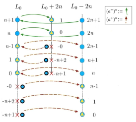
Figure 1: The diagram shows the shifted harmonic oscillators $L_{0}\pm 2n$ as super-partners of $L_{0}$. Symbol X indicates non-physical seed states $\psi_{-k}$, blue discs with boldface border indicate non-physical states $\widetilde{\psi_{-k}}$, see Eq. (2.6), and circles with inscribed yellow triangles indicate physical seed states $\psi_{n}$. Action of the corresponding intertwining operators is shown by arrows.

From the diagram it is easy to reed the spectrum of the corresponding superextended system. If we chose $\breve{L}=L_{0}+2n$, the intertwining operator $(a^{-})^{n}$ annihilates the first $n$ physical states of $L_{0}$, and the superextended system $(L_{0},L_{0}+2n)$ has $n$ singlet eigenstates given by $(\psi_{j},0)^{t}$ with $j=0,\ldots,n-1$. On the other hand, taking $(a^{+})^{n}$ as intertwining operator, we generate the superextended system $(L_{0},L_{0}-2n)$ characterized by $n$ singlet states $(0,\psi_{j})^{t}$. In correspondence with these arguments, the intertwining operators of the form $A_{(\pm)}^{-}(a^{\pm})^{n}$ and $A_{(\pm)}^{-}(a^{\mp})^{n}$ have the following interpretation: we first shift the initial system as much as we want with the corresponding power of $a^{\pm}$, and then we produce the nontrivial deformation. As a result, the final superextended system will present singlet states in correspondence with this shift. To illustrate the process, consider the two examples presented diagrammatically in Figure 2.

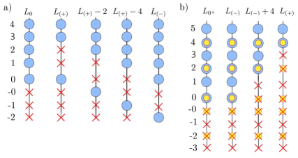
Figure 2: The diagrams show some modifications of the systems discussed in this section. On the left panel $a)$, the operator $L_{(+)}=L_{(-)}-6$, and $L_{(-)}$ is given by (5.19). On the right panel $b)$, the operator $L_{(-)}$ is defined in (5.1), and $L_{(+)}=L_{(-)}-8$. Circles with smaller yellow circles inside indicate even states which are non-physical eigenstates; small yellow crossed circles correspond to non-physical Wick-rotated even eigenstates.

This diagram follows the same logic of Fig. 1, but without showing the action of intertwining operators. According to the left panel a) of Fig. 2, one can construct the following super-extensions. By matching $L_{0}$ with $L_{(+)}$, we have the positive scheme discussed at the end of the previous subsection. Matching $L_{0}$ with $L_{(+)}-2$ results in the system with two singlet states of the form $(0,\psi_{n})^{t}$ with $n=0,1$, and one more singlet of the form $(\phi_{0},0)^{t}$, where $\phi_{0}$ is the ground state of $L_{(+)}$. By matching $L_{0}$ with $L_{(+)}-4$, we obtain the system with singlet states $(0,\psi_{0})$ and $(\phi_{0},0)^{t}$. Finally, by matching $L_{0}$ with $L_{(+)}-6=L_{(-)}$, we reproduce the negative scheme. In all these cases we use the chain of relations

$$\phi_{0}=A_{(+)}^{-}(a^{+})^{3}\widetilde{\psi_{-2}}=A_{(+)}^{-}(a^{+})^{2}\widetilde{\psi_{-1}}=A_{(+)}^{-}(a^{+})\widetilde{\psi_{-0}}=A_{(+)}^{-}\psi_{0}=A_{(-)}^{-}\widetilde{\psi_{-2}}$$

to be equalities modulo numerical multiplicative factors. A similar analysis can be done for deformations of the $L_{1}^{iso}$ with the help of the right panel b).

Any of these shifted deformed systems can be paired each other as super-partners. For example, we can pair $L_{(+)}$ and $L_{(-)}$ from panel a), and the intertwining operator for them will be the operator $\mathfrak{C}_{3}^{\pm}$. In this sense, each deformed system of a class $c$ can be paired with its proper copy but with the Hamiltonian displaced for additive constant $2cj$, $j=1,2,\ldots$, by using $\mathfrak{A}_{cj}^{\pm}$, $\mathfrak{B}_{cj}^{\pm}$, or $\mathfrak{C}_{cj}^{\pm}$ as intertwining operators.

6 Discussion and outlook

In conclusion, we indicate some open problems to be interesting for further investigation.

We considered super-extensions of rationally deformed harmonic oscillator and AFF models paired, respectively, with the undeformed harmonic or half-harmonic oscillator systems. But one could construct superextended systems composed from the pairs of rationally deformed systems having in mind that the corresponding dual schemes can be interpreted as periodic Darboux chains [60], in which the harmonic oscillator will just be an intermediate system between $L_{(-)}$ and $L_{(+)}$. In the corresponding superextended Hamiltonian (2.3) we then will have $\breve{L}=L_{(+)}$ and $L=L_{(-)}$, for which the intertwining operators are given by the sets of the ladder operators of the three families considered here. Such a generalization was discussed very schematically in Section 5.3. The use of some singular systems in the middle of the Darboux chain could allow to construct intertwining operators of less order. Situation like that appears in the case of exotic supersymmetry in finite-gap systems obtained from the free particle [36].

Recently, the $\mathcal{PT}$-regularized systems (3.1) with special values of the coupling constant $g=n(n+1)$ but without the confining potential term were studied in [39, 40] together with their rational deformations, which are intimately related to the Korteweg-de Vries hierarchy of completely integrable systems. It was found there that such systems reveal unusual properties, in particular, in the context of superconformal symmetries. It would be interesting to investigate the $\mathcal{PT}$-regularized versions of the superextended rationally deformed AFF systems studied by us here. We note that the $\mathcal{PT}$-regularized version of the undeformed model (3.1) was considered earlier in [10]. The indicated problem also is interesting in another aspect. If in the $\mathcal{PT}$-regularized AFF model we reconstruct the frequency parameter $\omega$ and consider the limit $\omega\rightarrow 0$, we reproduce the completely invisible zero-gap systems with $g=n(n+1)$ investigated in Refs. [39, 40]. Based on certain ladder operators we studied here, one can also reproduce the higher derivative Lax-Novikov integrals which underly peculiar properties of the systems from [39, 40]. However, in the same naïvely applied limit $\omega\rightarrow 0$ additional terms appearing in the rationally deformed versions of the AFF model turn into zero. Therefore, the question is whether the rational terms responsible, in particular, for the origin of the extreme wave solutions in [39] can be reproduced from the rational terms we have here by considering limit $\omega\rightarrow 0$ in some indirect way.

We were dealing here only with rationally deformed AFF models with special coupling constant values $g=n(n+1)$. It would be interesting to extend our analysis for the case of rational deformations of the AFF model of general form (3.1). For this, it will be necessary to generalize the three families of the ladder operators for the case of arbitrary values of the parameter $\nu$. Some rational deformations of the system (3.1) with arbitrary coupling constant values were considered in [14]. If the technique of dual schemes can be generalized for the case of $\nu\in\mathbb{R}$, our approach can also be extended for rational deformations of the AFF model (3.1). Some preliminary considerations indicate that this indeed can be done. In this context the case of gapless deformations is of a special interest due to their complete isospectrality to the original system (3.1) with corresponding value of the parameter $\nu$, which attracted considerable interest in the physics of anyons some time ago [61, 62]. This also could shed a light on the properties of the $\mathcal{PT}$-regularized two-particle Calogero systems with arbitrary values of $g=\nu(\nu+1)$ but without the confining potential term. One can expect that they have to be essentially different from the peculiar properties of the class of such systems with $g=n(n+1)$ studied in [39, 40].

Deformed superconformal symmetry we investigated is based essentially on the higher-derivative integrals of motion. Such integrals are associated usually with the hidden symmetries [18]. In their study, the Eisenhart-Duval lift [63, 64, 65, 66] plays a very important role by allowing to look at the system from the perspective of Riemannian geometry and to establish relation between different systems possessing hidden symmetries. It would be very interesting to consider the systems we studied by applying to them the method of the Eisenhart-Duval lift.

Acknowledgements

L.I. acknowledges the CONICYT scholarship 21170053 and the project FCI-PM-02 (USACH).

Appendix

Appendix A Operator identities (4.10)

We have equalities $\ker\,(A_{(-)}^{+}A_{(+)}^{-})=\Delta_{+}\cup\tilde{\delta}=\{0,1,\ldots,n\}$, where $\tilde{\delta}=\{A_{(-)}^{+}A_{(+)}^{-}\widetilde{\psi_{-l_{1}}},\ldots,\\ A_{(-)}^{+}A_{(+)}^{-}\widetilde{\psi_{-l_{n_{-}}}}\}$, and relation $\mathbb{A}_{(+)}^{+}\mathbb{A}_{(-)}^{-}\varphi_{n}\propto(a^{+})^{N}\varphi_{n}$ following from (4.6) is used. The first identity from (4.10) follows then from equality $\ker A_{(-)}^{+}A_{(+)}^{-}$ =$\ker(a^{-})^{N}$ [15].

In the second relation in (4.10), functions $f(\eta)$ and $h(\eta)$ are the polynomials

$$f(\eta)\equiv\prod_{l^{-}_{k}-n_{+}<0}(\eta+2l^{-}_{k}+1),\qquad h(\eta)\equiv\prod_{\check{n}^{-}_{k}-n_{+}\geq 0}(\eta+2\check{n}^{-}_{k}+1)\,,$$ (A.1)

where $l^{-}_{k}\in\Delta_{-}$ and $\check{n}^{-}_{k}$ are the absent states in $\Delta_{-}$. Using the mirror diagram technique [17], we obtain the equality $\ker f(L_{(-)})A_{(+)}^{-}(a^{+})^{n_{-}}=\ker h(L_{(-)})A_{(-)}^{-}(a^{-})^{n_{+}}$, where

$$\small{\begin{array}[]{rr}\ker f(L_{(-)})A_{(+)}^{-}(a^{+})^{n_{-}}=&\text{span}\{0,\ldots,(n_{+}-1),-0,\ldots,-(n_{-}-1),\\ &\qquad\qquad\{\widetilde{(\check{n}_{i}^{+}-n_{+})}\},\{-\widetilde{(\check{n}_{j}^{-}-n_{-})}\}\ \}\,.\end{array}}$$ (A.4)

Indexes $i$ and $j$ are running here over the absent states of both schemes, provided the conditions $\check{n}_{i}^{+}-n_{+}\geq 0$ and $\check{n}_{j}^{-}-n_{-}\geq 0$ are met. A special case corresponds to the positive scheme $\Delta_{+}=(l_{1}^{+},l_{1}^{+}+1,\ldots,l_{1}^{+}+q)$, for which the dual negative scheme is $\Delta_{-}=(-(q+1),\ldots,-(q+l_{1}^{+}))$. Here $n_{+}=1+q$ and $n_{-}=l_{1}^{+}$, there are no states to construct polynomials (A.1), and we just put $f(\eta)=h(\eta)=1$. Analogously, there are eigenstates with tilde in (A.4) in this case. In particular, if $n_{+}$ is an even number, then the DCKA transformation will produce a deformed harmonic oscillator with one gap of size $2(l_{1}^{-}+q+1)=2N$ in its spectrum, while if $q$ is an odd number and $l_{1}^{+}=1$, then we generate a gapless deformation of $L_{1}^{iso}$ (by introducing the potential barrier at $x=0$).

Appendix B Relations between symmetry generators

We first show explicitly how the three families appear by considering the commutators

$$\small{\begin{array}[]{l}[\mathfrak{C}_{N+l}^{-},\mathfrak{A}_{k}^{-}]=P_{n_{-}}(\eta)|_{\eta=L_{(+)}}^{\eta=L_{(+)}+2k}\mathfrak{C}_{N+k+l}^{-}\,,\qquad[\mathfrak{C}_{N+l}^{+},\mathfrak{B}_{k}^{+}]=P_{n_{-}}(\eta)|_{\eta=L_{(+)}}^{\eta=L_{(-)}-2l}\mathfrak{C}_{N+k+l}^{+}\,,\\ {}[\mathfrak{A}_{k}^{+},\mathfrak{C}_{N+l}^{-}]=(-1)^{n_{-}}T_{k}(L_{(-)})\mathfrak{A}_{N+l-k}^{-}-P_{n_{-}}(L_{(+)})T_{l}(L_{(+)}+2l)\mathfrak{C}_{N+l-k}^{-}\,,\\ {}[\mathfrak{B}_{k}^{-},\mathfrak{C}_{N+l}^{+}]=(-1)^{n_{-}}T_{k}(L_{(+)}+2k)\mathfrak{B}_{N+l-k}^{+}-T_{l}(L_{(-)})P_{n_{+}}(L_{(-)}-2l)\mathfrak{C}_{N+l-k}^{+}\,,\\ {}[\mathfrak{C}_{N+k}^{+},\mathfrak{C}_{N}^{-}]=P_{n_{+}}(L_{(-)}-2k)\mathfrak{A}_{k}^{-}-P_{n_{-}}(L_{(-)}+2N)\mathfrak{B}_{k}^{-}\,,\\ {}[\mathfrak{C}_{N\pm k}^{\pm},\mathfrak{C}_{N\pm l}^{\pm}]=0\,,\qquad\l\geq 0\,,\end{array}}$$ (B.6)

where polynomials $P_{n_{\pm}}(\eta)$ and $T_{k}(\eta)$ are defined by Eqs. (4.8) and (4.9). These commutators should be interpreted as recursive relations which generate the elements of the three families of the ladder operators proceeding from the spectrum generating set of operators with $l=r(N,c)$ and $k=c$. On the other hand, the commutators of the ladder operators with their own conjugate counterparts are

$$\small{\begin{array}[]{c}[\mathfrak{A}_{k}^{-},\mathfrak{A}_{k}^{+}]=P_{n_{-}}(\eta-2k)P_{n_{-}}(\eta)T_{k}(\eta)|_{\eta=L_{(-)}}^{\eta=L_{(-)}+2k}\,,\\ \,[\mathfrak{B}_{k}^{-},\mathfrak{B}_{k}^{+}]=P_{n_{+}}(\eta-2k)P_{n_{+}}(\eta)T_{k}(\eta)|_{\eta=L_{(+)}}^{\eta=L_{(+)}+2k}\,,\\ \,[\mathfrak{C}_{N\pm k}^{-},\mathfrak{C}_{N\pm k}^{+}]=P_{n_{-}}(\eta)P_{n_{+}}(x-2k)T_{k}(\eta)|_{\eta=L_{(-)}}^{\eta=L_{(+)}\pm 2k}\,.\end{array}}$$ (B.10)

In this way, we obtain a deformation of $sl(2,\mathbb{R})$ in (4.13).

Below we present some relations between lowering ladder operators, from which analogous relations for raising operators can be obtained via Hermitian conjugation.

The definitions of the three families automatically provide the following relations:

$$\mathfrak{A}_{N+k}^{-}=(-1)^{n_{-}}P_{n_{-}}(L_{(-)})\mathfrak{C}_{N+k}^{-}\,,\qquad\mathfrak{B}_{N+k}^{-}=(-1)^{n_{-}}\mathfrak{C}_{N+k}^{-}P_{n_{+}}(L_{(+)}),$$ (B.11)

$$\mathfrak{C}_{N-(N+k)}^{-}\equiv\mathfrak{C}_{-k}^{-}=(-1)^{n_{-}}P_{n_{+}}(L_{(-)}+2N)\mathfrak{A}_{k}^{+}\,,$$ (B.12)

$$\mathfrak{C}_{2N+l+k}^{-}=(-1)^{n_{-}}\mathfrak{C}_{N+l}^{-}\mathfrak{C}_{N+k}^{-}\,,$$ (B.13)

$$(\mathfrak{C}_{N+k}^{-})^{2}=(-1)^{n_{-}}\mathfrak{C}_{2N+2k}^{-}\,,$$ (B.14)

where $k,l=0,1,\ldots$. Eq. (B.11) means that operators of families $\mathfrak{A}$ and $\mathfrak{B}$ with index $k\geq N$ are essentially the operators of the $\mathfrak{C}$ family. Eq. (B.12) shows that operators of the form $\mathfrak{C}_{-k}^{\pm}$ are not basic. If in (B.13) one fixes $l=r(N,c)$, then all the operators with index equal or greater than $N+r(N,c)$ reduce to the products of the basic elements. Finally, Eq. (B.14) means that the square of an operator of $\mathfrak{C}$-family with odd index $N+k$ is a physical operator, but not basic. The unique special case is when $c=2$, $N$ is odd, and $k=0$ since there is no product of physical operators of lower order which could make the same job. From here we conclude that the basic operators are given by (4.11).

For one-gap system we can use the second equation in (4.10) (where $f(\eta)=h(\eta)=1$) to find some relations between operators with indexes less than $N$ :

$$\small{\begin{array}[]{ll}\mathfrak{C}^{-}_{n_{+}-k}=(-1)^{n_{-}}\mathfrak{A}_{n_{+}-k}^{-}T_{k}(L_{(-)})\,,&\mathfrak{C}^{-}_{n_{-}-k^{\prime}}=(-1)^{n_{-}}\mathfrak{B}_{n_{-}-k^{\prime}}^{-}T_{k^{\prime}}({L_{(-)}}+2(n_{+}-k^{\prime}))\,,\\ \mathfrak{A}_{n_{+}+k^{\prime}}^{-}=(-1)^{n_{-}}\mathfrak{C}_{n_{+}+k^{\prime}}^{-}T_{k^{\prime}}(L_{(-)})\,,&\mathfrak{B}_{n_{-}+k}^{-}=(-1)^{n_{-}}\mathfrak{C}_{n_{-}+k}^{-}T_{k}(L_{(-)}+2n_{+})\,,\end{array}}$$ (B.17)

where $k=0,\ldots,n_{+}$ and $k^{\prime}=0,\ldots,n_{-}$. By considering the ordering relation between $n_{-}$ and $n_{+}$, we can combine relations (B.17) to represent operators of the $\mathfrak{A}$ family in terms of $\mathfrak{B}$ family or vice versa. For the case $n_{-}<n_{+}$ we have

$$\mathfrak{B}_{n_{+}-k}^{-}=T_{(n_{+}-n_{-}-k)}(L_{(-)}+4n_{+}-2k)T_{k}(L_{(-)}+2n_{+})\mathfrak{A}_{n_{+}-k}^{-}\,,$$ (B.18)

where $k=0,\ldots,n_{+}-n_{-}$. In other words, only first $n_{-}-1$ operators are basic. In the case $n_{-}=1$, there exist no basic elements in the $\mathfrak{B}$-family. As examples corresponding to this observation we have all the deformations produced by a unique non-physical state of the form $\psi_{-n}(x)$. On the other hand, in the case $n_{+}<n_{-}$ we have

$$\mathfrak{A}_{n_{-}-k}^{-}=T_{k}(L_{(-)}+2N)T_{(n_{-}-n_{+}-k)}(L_{(-)}+2(n_{-}-k))\mathfrak{B}_{n_{-}-k}^{-}\,,$$ (B.19)

where $k=0,\ldots,n_{-}-n_{+}$. According to this, only first $n_{+}-1$ elements cannot be written in terms of the operators of $\mathfrak{B}$ family. The unique case in which there exist no basic elements of the families $\mathfrak{A}$ or $\mathfrak{B}$ is when $n_{-}=n_{+}=1$, which corresponds to the shape invariance of the harmonic oscillator. As a final result, the basic elements of the three families are given by (4.23).

We consider now the relations between Darboux generators $A_{(\pm)}^{-}(a^{\pm})^{n}$ and $A_{(\pm)}^{-}(a^{\mp})^{n}$. Using the first relation in (4.10) and the definition of operators $\mathfrak{C}_{N+l}^{\pm}$, we obtain relations

$$A_{(-)}^{-}(a^{-})^{N+l}=(-1)^{n_{-}}P_{n_{-}}(L_{(-)})A_{(+)}^{-}(a^{-})^{l}\,,\quad A_{(+)}^{-}(a^{+})^{N+l}=(-1)^{n_{-}}P_{n_{+}}(L_{(+)})A_{(-)}^{-}(a^{+})^{l}\,,$$

$$A_{(+)}^{-}(a^{-})^{N+l+k}=(-1)^{n_{-}}\mathfrak{C}_{N+l}^{-}A_{(+)}^{-}(a^{-})^{k}\,,\quad A_{(-)}^{-}(a^{+})^{N+l+k}=(-1)^{n_{-}}\mathfrak{C}_{N+l}^{+}A_{(-)}^{-}(a^{+})^{k}\,,$$

where $k,l=0,1,2,\ldots$. If we fix $l=r(N,c)$, then one finds that the basic elements are just (4.26). On the other hand for one gap-systems, with the help of (4.10) one can obtain relations

$$A_{(-)}^{-}(a^{-})^{n_{+}+k}=(-1)^{n_{-}}A_{(+)}(a^{+})^{n_{-}-k}T_{k}(L)\,,$$ (B.20)

$$A_{(+)}^{-}(a^{+})^{n_{-}+k^{\prime}}=(-1)^{n_{-}}A_{(-)}^{-}(a^{-})^{n_{+}-k^{\prime}}T_{k^{\prime}}(L+2k^{\prime})\,,$$ (B.21)

with $k=0,\ldots,n_{-}$ and $k^{\prime}=0,\ldots,n_{+}$. These relations reduce the basic subsets of Darboux generators to (4.27).

Appendix C (Anti)-Commutation relations for one-gap system

In this Appendix we summarize some (anti)commutation relations for one-gap deformations of harmonic oscillator systems.

For the anticommutator of two fermionic operators in (4.31) we have

$$\mathbb{P}_{z}=\small{\left\{\begin{array}[]{lcc}P_{n_{-}}(\eta)T_{|z|}(\eta)\big{|}_{\eta=\mathcal{H}+2|z|\Pi_{-}+\lambda_{-}}&-N<z\leq 0\\ \vspace{-0.4cm}\\ P_{n_{-}}(\eta)T_{z}(\eta+2z)\big{|}_{\eta=\mathcal{H}-2|z|\Pi_{-}+\lambda_{-}}&0<z\leq n_{+}\\ \end{array}\right.\,,}$$ (C.4)

and for the positive scheme

$$\mathbb{P}^{\prime}_{z}=\small{\left\{\begin{array}[]{lcc}P_{n_{+}}(\eta)T_{|z|}(\eta-2z)\big{|}_{\eta=\mathcal{H}^{\prime}-2|z|\Pi_{-}+\lambda_{+}}&-N<z\leq 0\\ \vspace{-0.4cm}\\ P_{n_{+}}(\eta)T_{z}(\eta)\big{|}_{\eta=\mathcal{H}^{\prime}+2|z|\Pi_{-}+\lambda_{+}}&0<z\leq n_{-}\\ \end{array}\right.\,.}$$ (C.8)

By virtue of the relation between dual schemes, the expression $\mathbb{P}^{\prime}_{z}(\mathcal{H}^{\prime},\sigma_{3})=\mathbb{P}_{N-z}(\mathcal{H}^{\prime}+N(1+\sigma_{3})-\lambda_{-}+\lambda_{+},\sigma_{3})$ helps to complete the set of polynomials.

For the negative scheme we also have

$$[\mathcal{G}_{-k}^{(2\theta(z)-1)},\mathcal{Q}_{a}^{0}]=\frac{1}{2}P_{n_{-}}(\eta)|_{\eta=\mathcal{H}+\lambda_{-}}^{\eta=\mathcal{H}+\lambda_{-}+2|z|}(\mathcal{Q}_{a}^{z}-(2\theta(z)-1)i\epsilon_{ab}\mathcal{Q}_{b}^{z})\,,\qquad$$ (C.9)

where $z\in(-N,0)\cup(0,2N)$, while for the positive scheme, where $\mathcal{Q}_{a}^{{}^{\prime}z}=\mathcal{Q}_{a}^{N-z}$ and $\mathcal{G}_{\pm k}^{{}^{\prime}(1)}=\mathcal{G}_{\pm k}^{(1)}$ when $k\geq N$, we have

$$[\mathcal{G}_{-z}^{{}^{\prime}(2\theta(z)-1)},\mathcal{Q}_{a}^{{}^{\prime}0}]=\frac{1}{2}P_{n_{+}}(x)|_{x=\mathcal{H}^{\prime}+\lambda_{+}}^{x=\mathcal{H}^{\prime}+\lambda_{+}+2|z|}(\mathcal{Q}_{a}^{{}^{\prime}z}+(2\theta(z)-1)i\epsilon_{ab}\mathcal{Q}_{b}^{{}^{\prime}z})\,,$$ (C.10)

where $z\in(-N,0)\cup(0,2N)$. On the other hand, for the negative scheme the relation $[\mathcal{G}_{z}^{(1)},\mathcal{Q}_{a}^{z}]=\frac{\mathcal{V}_{z}(\mathcal{H})}{2}(\mathcal{Q}_{a}^{0}+i(2\theta(z)-1)\epsilon_{ab}\mathcal{Q}_{b}^{0})\,$ is valid, where

$$\mathcal{V}_{z}=\left\{\begin{array}[]{lcc}P_{n_{-}}(\eta)T_{z}(\eta)\big{|}^{\eta=\mathcal{H}+\lambda_{-}-2z}_{\eta=\mathcal{H}+\lambda_{-}}\,,&-N<z<0\,,\\ \vspace{-0.4cm}\\ P_{n_{-}}(\eta)T_{z}(\eta+2z)\big{|}^{\eta=\mathcal{H}+\lambda_{-}}_{\eta=\mathcal{H}+\lambda_{-}-2z}\,,&0<z\leq n_{+}\,,\\ \vspace{-0.4cm}\\ P_{n_{+}}(\eta)T_{N-z}(\eta)\big{|}^{\eta=\mathcal{H}+\lambda_{-}+2N}_{\eta=\mathcal{H}+\lambda_{-}+2(N-z)}\,,&n_{+}<z\leq N\,,\\ \vspace{-0.4cm}\\ P_{n_{+}}(\eta)T_{z}(\eta+2z)\big{|}^{\eta=\mathcal{H}+\lambda_{-}+2N}_{\eta=\mathcal{H}+\lambda_{-}-2z}\,,&N<z<2N\,.\end{array}\right.$$ (C.18)

In the positive scheme we have $[\mathcal{G}_{z}^{{}^{\prime}(1)},\mathcal{Q}_{a}^{{}^{\prime}z}]=\frac{\mathcal{V}_{z}^{\prime}(\mathcal{H}^{\prime})}{2}(\mathcal{Q}_{a}^{{}^{\prime}0}-i(2\theta(z)-1)\epsilon_{ab}\mathcal{Q}_{b}^{{}^{\prime}0})$, where $\mathcal{V}_{z}^{\prime}(\mathcal{H}^{\prime})$ are given by

$$\mathcal{V}_{z}^{\prime}=\left\{\begin{array}[]{lcc}P_{n_{+}}(\eta)T_{z}(\eta+2z)\big{|}^{\eta=\mathcal{H}^{\prime}+\lambda_{+}}_{\eta=\mathcal{H^{\prime}}+\lambda_{+}-2z}\,,&-N<z<0\,,\\ \vspace{-0.4cm}\\ P_{n_{+}}(\eta)T_{z}(\eta)\big{|}^{\eta=\mathcal{H}^{\prime}+\lambda_{+}}_{\eta=\mathcal{H}^{\prime}+\lambda_{+}}\,,&0<z\leq n_{-}\,,\\ \vspace{-0.4cm}\\ P_{n_{-}}(\eta-2N)T_{N-z}(\eta-2z)\big{|}^{\eta=\mathcal{H}^{\prime}+\lambda_{+}+2z}_{\eta=\mathcal{H}^{\prime}+\lambda_{+}}\,,&n_{-}<z\leq N\,,\\ \vspace{-0.4cm}\\ P_{n_{-}}(\eta)T_{z}(\eta)\big{|}^{\eta=\mathcal{H}^{\prime}+\lambda_{+}+2z}_{\eta=\mathcal{H}^{\prime}+\lambda_{+}-2N}\,,&N<z<2N\,.\end{array}\right.$$ (C.26)

These are the missing relations which prove that the subsets $\mathcal{U}_{0,z}^{(2\theta-1)}$ defined in (4.46), satisfy closed superalgebras independently of choosing the scheme. On the other hand, we can use them to prove that the subsets $\mathcal{I}_{N,z}^{(2\theta-1)}$ given in (4.48) also produce closed superalgebras. Other useful relations are

$$[\mathcal{G}_{-(N+l)}^{(1)},\mathcal{Q}_{a}^{N+k}]=\frac{1}{2}T_{k}(\eta)P_{n_{+}}(\eta+2k)|_{\eta=\mathcal{H}+\lambda_{-}}^{\eta=\mathcal{H}+\lambda_{-}+2(N-k)}(\mathcal{Q}_{a}^{l-k}+i\epsilon_{ab}\mathcal{Q}_{b}^{l-k})\,,$$ (C.27)

where $l>k$ and $l-k\leq n_{+}$. For $l<k$ we have

$$[\mathcal{G}_{-(N+l)}^{(1)},\mathcal{Q}_{a}^{N+k}]=P_{n_{-}}(\mathcal{H}+\lambda_{-})(\mathcal{Q}_{a}^{k-l}+i\epsilon_{ab}\mathcal{Q}_{b}^{k-l})\,,$$ (C.28)

and also we can write $[\mathcal{G}_{\pm(N\pm k)}^{(1)},\mathcal{G}_{\pm(N\pm l)}^{(1)}]=0$ for any values of $k$ and $l$.

Appendix D List of polynomial functions for Section 5.2

Eq. (5.25) : $P_{\alpha,\beta}(\mathcal{H})=-P_{-\alpha,-\beta}(\mathcal{H}-2(\alpha+\beta))$, and

$$\small{\begin{array}[]{lll}P_{-1,1}=\mathcal{H}(6\mathcal{H}-20)-8\Pi_{-}(\mathcal{H}-3)\,,&P_{-1,-2}=-2\mathcal{H}+12(1-\Pi_{-})\,,&P_{-1,+2}=10(\mathcal{H}-4)-12\Pi_{-}\,,\\ M_{-1,+2}=12\,,&P_{-1,-3}=P_{-2,-3}=-6\,,&P_{-1,+3}=-12\,,\\ M_{-1,+3}=24\,,&P_{-1,-4}=P_{-2,-4}=-8\,,&P_{-1,+4}=16(\mathcal{H}-5-\Pi_{-})\,,\\ P_{-1,-5}=P_{-2,-5}=-10\,,&P_{-1,+5}=20(\mathcal{H}-6-\Pi_{-})\,,&\end{array}}$$ (D.5)

$$\small{\begin{array}[]{ll}P_{-2,+2}=(\mathcal{H}-4)[8\mathcal{H}(2\mathcal{H}-7)+\Pi_{-}(4\mathcal{H}^{2}-44\mathcal{H}+192)]\,,&P_{-2,+3}=-18\mathcal{H}+96-4(\mathcal{H}-30)\Pi_{-}\,,\\ M_{-2,+3}=M_{-2,+4}=-96\,,&P_{-2,+4}=-2(11\mathcal{H}-\Pi_{-})+136\,,\\ P_{-2,+5}=1104-340\mathcal{H}+26\mathcal{H}^{2}+\Pi_{-}(576-104\mathcal{H}+10\mathcal{H}^{2})\,,&P_{-3,+4}=24\mathcal{H}-144+\Pi_{-}(2\mathcal{H}-76)\,,\\ M_{-3,+4}=848\,,&P_{-3,+5}=30\mathcal{H}-180+\Pi_{-}(8\mathcal{H}-180)\,,\\ M_{-3,+5}=960\,,\\ P_{-4,+5}=40(32-10\mathcal{H}+\mathcal{H}^{2}-\Pi_{-}(7\mathcal{H}-32))\,,&M_{-4,+5}=-5760\,,\\ \end{array}}$$ (D.12)

$$\small{\begin{array}[]{l}P_{-4,+4}=4[7\mathcal{H}^{3}-56\mathcal{H}^{2}+116\mathcal{H}+32+\Pi_{-}(\mathcal{H}^{3}-64\mathcal{H}^{2}+572\mathcal{H}+1472)]\,,\\ P_{-5,+5}=2(320-2848\mathcal{H}+1268\mathcal{H}^{2}-248\mathcal{H}^{3}+23\mathcal{H}^{4})+\\ \qquad\qquad\qquad 8\Pi_{-}(10000-6212\mathcal{H}+1492\mathcal{H}^{2}-187\mathcal{H}^{3}+12\mathcal{H}^{4})\,.\end{array}}$$ (D.16)

Eq. (5.26) : $F_{\alpha,\beta}(\mathcal{H})=-F_{-\alpha,-\beta}(\mathcal{H}-2(\alpha+\beta))$, and

$$\small{\begin{array}[]{lll}F_{+1,-1}=F_{-1,+3}=0\,,&N_{+1,-1}=-F_{-1,-2}=-N_{-2,+1}=2\,,&F_{-2,-1}=F_{-2,-2}=-4\,,\\ F_{-1,+2}=-N_{-1,+3}=6\,,&F_{-1,+4}=F_{-2,+1}=8\,,&F_{-1,+5}=10\,,\\ N_{-1,+2}=F_{-2,+3}=-12\,,&F_{-2,+4}=-16&N_{-2,+3}=N_{-2,+4}=48\,,\\ F_{-1,+1}=4(\mathcal{H}-3)\,,&F_{-2,+5}=24(\mathcal{H}-7)\,,&F_{-2,+2}=12(\mathcal{H}-4)^{2}\,,\end{array}}$$ (D.21)

while other elements are zero.

Eq. (5.30) : $\mathbb{C}_{\alpha,\beta}=\mathbb{C}_{\beta,\alpha}$ , and

$$\small{\begin{array}[]{ll}\mathbb{C}_{-2,-1}=\mathcal{G}_{+1}^{(1)}(\mathcal{H}-6)+8\mathcal{G}_{+1}^{(0)}\,,&\mathbb{C}_{-2,0}=\mathcal{G}_{-2}^{(1)}+4\mathcal{G}_{-2}^{(0)}\,,\\ \mathbb{C}_{-2,1}=-(\mathcal{H}-4\Pi_{-})\mathcal{G}_{-3}^{(1)}\,,&\mathbb{C}_{-2,2}=(\mathcal{H}+4\Pi_{-})\mathcal{G}_{-4}^{(1)}\,,\\ \mathbb{C}_{-2,5}=\mathcal{G}_{-7}^{(1)}=-\mathcal{G}_{-3}^{(1)}\mathcal{G}_{-4}^{(1)}\,,&\mathbb{C}_{-1,0}=\mathcal{G}_{-1}^{(1)}+\mathcal{G}_{-1}^{(0)}\,,\\ \mathbb{C}_{-1,1}=-\mathcal{G}_{-2}^{(1)}+2\mathcal{G}_{-2}^{(0)}\,,&\mathbb{C}_{-1,4}=\mathcal{G}_{-5}^{(1)}\,,\\ \mathbb{C}_{-1,5}=\mathcal{G}_{-6}^{(1)}=-(\mathcal{G}_{-2}^{(1)})^{2}\,,&\mathbb{C}_{1,2}=-(\mathcal{H}-2)(\mathcal{G}_{-1}^{(1)}+6\mathcal{G}_{-1}^{(0)})\,,\\ \mathbb{C}_{1,3}=-\mathcal{G}_{-2}^{(1)}+6\mathcal{G}_{-2}^{(0)}\,,&\mathbb{C}_{1,4}=(\mathcal{H}-4\sigma_{3})\mathcal{G}_{-3}^{(1)}\,,\\ \mathbb{C}_{1,5}=(\mathcal{H}-4-10\Pi_{-})\mathcal{G}_{-4}^{(1)}\,,&\mathbb{C}_{2,3}=(\mathcal{H}-2)\mathcal{G}_{-1}^{(1)}-12(\mathcal{H}-4)\mathcal{G}_{-1}^{(0)}\,,\\ \mathbb{C}_{2,4}=(\mathcal{H}-2)\mathcal{G}_{-2}^{(1)}-16(\mathcal{H}+3)\mathcal{G}_{-2}^{(0)}\,,&\mathbb{C}_{2,5}=((\mathcal{H}-2)(\mathcal{H}-4)-8(\mathcal{H}-5)\Pi_{-})\mathcal{G}_{-3}^{(1)}\,,\\ \mathbb{C}_{3,4}=(\mathcal{H}-2)\mathcal{G}_{-1}^{(1)}-16(\mathcal{H}-5)\mathcal{G}_{-1}^{(0)}\,,&\mathbb{C}_{3,5}=-(\mathcal{H}+2)\mathcal{G}_{-2}^{(1)}-20(\mathcal{H}-4)\mathcal{G}_{-2}^{(0)}\,,\\ \end{array}}$$ (D.31)

$$\small{\begin{array}[]{l}\mathbb{C}_{4,5}=[(\mathcal{H}-2)(\mathcal{H}+6)-2\Pi_{-}(12\mathcal{H}-117))\mathcal{G}_{-1}^{(1)}-720\mathcal{G}_{-1}^{(0)}\,.\end{array}}$$ (D.33)

Eq. (5.31) :

$$\small{\begin{array}[]{llll}\mathbb{Q}_{1,-2}^{1}=2\,,&\mathbb{Q}_{1,-2}^{2}=5\,,&\mathbb{Q}_{2,3}^{1}=7(40-\mathcal{H})\,,&\mathbb{Q}_{2,3}^{2}=-3\,,\\ \mathbb{Q}_{1,-2}^{1}=2\,,&\mathbb{Q}_{1,-2}^{2}=5(\mathcal{H}-4)\,,&\mathbb{Q}_{2,4}^{1}=-10(\mathcal{H}-6)\,,&\mathbb{Q}_{2,4}^{2}=-4\,,\\ \mathbb{Q}_{1,-1}^{1}=-1\,,&\mathbb{Q}_{1,-1}^{2}=3\mathcal{H}-10\,,&\mathbb{Q}_{2,5}^{1}=(336-118\mathcal{H}+11\mathcal{H}^{2})\,,&\mathbb{Q}_{2,5}^{2}=5\,,\\ \mathbb{Q}_{1,2}^{1}=5(\mathcal{H}-4)\,,&\mathbb{Q}_{1,2}^{2}=\mathcal{H}\,,&\mathbb{Q}_{3,1}^{1}=3\,,&\mathbb{Q}_{3,1}^{2}=1\,,\\ \mathbb{Q}_{1,3}^{1}=-10\,,&\mathbb{Q}_{1,3}^{2}=-6\,,&\mathbb{Q}_{3,2}^{1}=-8(\mathcal{H}-3)\,,&\mathbb{Q}_{3,2}^{2}=4\,,\\ \mathbb{Q}_{1,4}^{1}=7(\mathcal{H}-36)\,,&\mathbb{Q}_{1,4}^{2}=4\,,&\mathbb{Q}_{4,1}^{1}=2\,,&\mathbb{Q}_{4,1}^{2}=-1\,,\\ \mathbb{Q}_{1,5}^{1}=9(\mathcal{H}-56)\,,&\mathbb{Q}_{1,5}^{2}=5\,,&\mathbb{Q}_{4,2}^{1}=10(3-\mathcal{H})\,,&\mathbb{Q}_{4,2}^{2}=-5\,,\\ \mathbb{Q}_{2,-2}^{1}=-2\,,&\mathbb{Q}_{2,-2}^{2}=4(\mathcal{H}-4)(2\mathcal{H}-7)\,,&\mathbb{Q}_{5,1}^{1}=5\,,&\mathbb{Q}_{5,1}^{2}=3\,,\\ \mathbb{Q}_{2,-1}^{1}=-1\,,&\mathbb{Q}_{2,-1}^{2}=5(\mathcal{H}+2)\,,&\mathbb{Q}_{5,2}^{1}=6(\mathcal{H}-1)\,,&\mathbb{Q}_{5,2}^{2}=3\,.\\ \end{array}}$$ (D.43)

Eq. (5.32) :

$$\small{\begin{array}[]{llll}\mathbb{G}_{1,-2}^{1}=-1\,,&\mathbb{G}_{1,-2}^{2}=(8-\mathcal{H})\,,&\mathbb{G}_{2,-2}^{1}=-1\,,&\mathbb{G}_{2,-2}^{2}=(\mathcal{H}+8)(\mathcal{H}-6)\,,\\ \mathbb{G}_{1,-1}^{1}=1\,,&\mathbb{G}_{1,-1}^{2}=(4-\mathcal{H})\,,&\mathbb{G}_{2,-1}^{1}=1\,,&\mathbb{G}_{2,-1}^{2}=4-\mathcal{H}\,,\\ \mathbb{G}_{1,0}^{1}=\mathbb{G}_{1,0}^{2}=1\,,&\mathbb{G}_{2,0}^{1}=-\mathbb{G}_{2,0}^{2}=1\,,&\mathbb{G}_{1,1}^{1}=\mathcal{H}-4\,,&\mathbb{G}_{1,1}^{2}=-1\,,\\ \mathbb{G}_{2,1}^{1}=\mathcal{H}-2\,,&\mathbb{G}_{2,1}^{2}=\mathcal{H}\,,&\mathbb{G}_{1,2}^{1}=\mathcal{H}-4\,,&\mathbb{G}_{1,2}^{2}=\mathcal{H}\,,\\ \mathbb{G}_{2,2}^{1}=-1\,,&\mathbb{G}_{2,2}^{2}=\mathcal{H}\,,&\mathbb{G}_{1,3}^{1}=\mathbb{G}_{1,3}^{2}=-1\,,&\mathbb{G}_{2,3}^{1}=4-\mathcal{H}\,,\\ \mathbb{G}_{2,3}^{2}=-1\,,&\mathbb{G}_{1,4}^{1}=\mathcal{H}-4\,,&\mathbb{G}_{1,4}^{2}=-1\,,&\mathbb{G}_{2,4}^{1}=2-\mathcal{H}\,,\\ \mathbb{G}_{2,4}^{2}=1\,,&\mathbb{G}_{1,5}^{1}=\mathcal{H}-4\,,&\mathbb{G}_{1,5}^{2}=-1\,,&\mathbb{G}_{2,5}^{1}=(\mathcal{H}-2)(\mathcal{H}-4)\,,\\ \mathbb{G}_{2,5}^{2}=-1\,.\end{array}}$$ (D.52)