Chaos and Order in the Bitcoin Market

Abstract

The bitcoin price has surged in recent years and it has also exhibited phases of rapid decay. In this paper we address the question to what extent this novel cryptocurrency market can be viewed as a classic or semi-efficient market. Novel and robust tools for estimation of multi-fractal properties are used to show that the bitcoin price exhibits a very interesting multi-scale correlation structure. This structure can be described by a power-law behavior of the variances of the returns as functions of time increments and it can be characterized by two parameters, the volatility and the Hurst exponent. These power-law parameters, however, vary in time. A new notion of generalized Hurst exponent is introduced which allows us to check if the multi-fractal character of the underlying signal is well captured. It is moreover shown how the monitoring of the power-law parameters can be used to identify regime shifts for the bitcoin price. A novel technique for identifying the regimes switches based on a goodness of fit of the local power-law parameters is presented. It automatically detects dates associated with some known events in the bitcoin market place. A very surprising result is moreover that, despite the wild ride of the bitcoin price in recent years and its multi-fractal and non-stationary character, this price has both local power-law behaviors and a very orderly correlation structure when it is observed on its entire period of existence.

Keywords: Bitcoin, Multi-fractality, Power Law, Regime Switching, Hurst Exponent, Volatility, Spectral Estimation
MSC[2010] 60G22, 62M09, 91Gxx

1 Introduction

Bitcoin is the main cryptocurrency and has been the subject of much interest, both from the point of view of speculation as well as from the point of view of the technology used in this market. In view of the success of the bitcoin market other cryptocurrencies have tried to copy their technology, but bitcoin remains the dominant technology with a market capitalization of about $40 billions in mid-2017. It is also interesting to understand this new market from a price or time series modeling viewpoint. It is the latter question that motivates this paper.

The bitcoin currency was launched in 2009. As a cryptocurrency it is not regulated via centralized banks, but rather transaction happens over decentralized computer networks and organized via block chain technology [1]. In the early years (2010-2013) bitcoin exchange was handled by Mt. Gox, an administration system based on Shibuya, Japan, handling about 70% of the transactions in late 2013. Then in early 2014 it became clear that Mt. Gox had been hacked resulting in a loss of bitcoins valued at about $450 millions. Complaints about delays in withdrawing cash from Mt. Gox were mounting in early 2014 and on 7 of February 2014 Mt. Gox halted all bitcoin withdrawals citing a bug in the bitcoin software that made hacking possible. The subsequent loss of confidence in the currency led to a rapid price drop. The confidence has, however, seemingly rebounded as several new exchange platforms have opened and the price surged to a high in early 2018 before a downward correction in the following months.

One may expect that the lack of centralized bank and regulatory agency means that the currency is very sensitive and volatile and not efficient in a classic sense. Moreover, one may expect that the price evolution after the announcement of the hacking of Mt. Gox was special reflecting a reduced confidence in this currency which may have persisted for some time. These are among the questions we want to examine in this paper.

The bitcoin market being the main cryptocurrency market has indeed been the subject of much research recently. This type of technology may change fundamentally the arena for financial transactions. In view of its unique role as a pointer to what may be to come in financial markets it is thus of great interest to see what kind of price structure and dynamics one finds in the bitcoin cryptocurrency market.

In [2] the authors analyze the bitcoin price with respect to multi-scale temporal correlation structure and relate this to the concept of chaos. They identify a low price period between July 2010 and February 2013 and a high price period from February 2013 till October 2017, by using a decomposition based on price level. A main conclusion presented in [2] is that chaos is present in the case of prices, but not for the returns. It is also found that heavy distribution tails are the main factor driving the chaos measure. The returns refer to the relative price changes over a certain time interval which typically corresponds to the sampling interval. The analysis in [2] is carried out partly via multi-fractal detrended fluctuation analysis where data over various scales and intervals are detrended and the associated residual moments of different orders are calculated [3]. A similar technique is used for cross-correlation analysis in [4]. In [5, 6] various types of detrended fluctuations analysis are used, however, with a moving window to track changes. The approach presented here regarding power law decay in time for correlations of returns is different from the approaches cited above, in particular in that we focus on the second-order moments, moreover, we do not carry out any detrending of the data.

We remark that a power law behavior of the bitcoin price was analyzed from a different perspective in [7], where the authors analyze a power law, or relatively slow, decay in the marginal distribution of the returns. This interesting study suggests a universal behavior and a power law decay of the marginal distribution with an exponent approximately equal to $2.5$. This value corresponds to heavier tail than in classic financial markets which typically exhibit an inverse cubic law of decay for the tail of the marginal distribution. Importantly this means in particular that the returns have a finite second moment. Here we discuss the issue of the marginal distribution of the returns in D where we show that our results are robust with respect to the presence of non-Gaussian returns distribution.

In our analysis we use an approach with a moving time window to track changes in the correlation structure. We focus on the correlation structure of the returns and set forth an approach based on this structure for detection of regime shifts. When we look at the returns in a time window we find a very interesting and orderly scaling of the second-order moments of the returns as functions of return time increments. The approach for segmentation is based on the residual relative to a fitted power law. What is quite surprising in our analysis is that the local power laws coexist with a global power law also on the entire period of bitcoin existence. In the classic Black-Scholes framework [8] the log-price is a standard Brownian motion so that the returns are stationary, independent, and Gaussian. We remark that under the risk-neutral or pricing measure, the drift of the log-price is the risk free interest rate which follows from a no-arbitrage or efficient market condition. Our focus here is, however, on the fluctuations of the returns, the Brownian part, whose statistical structure is the same under the risk-neutral measure and the physical measure corresponding to observed prices as considered here. To describe the considered power-law framework let $\Delta t$ be the time increment over which the returns are computed. We speak about power laws when the variances of the (zero-mean) returns are of the form $\sigma^{2}|\Delta t|^{2H}$, and we refer to $\sigma$ as the volatility and $H$ as the Hurst exponent. A classic model for such a power law is fractional Brownian motion [9]. Indeed, this model gives a generalization of the classic Black-Scholes model corresponding to the log return being standard Brownian motion with $H=1/2$. In the fractional Brownian motion case the returns are not independent, consecutive returns have a non-zero correlation coefficient of $\rho_{H}=(2^{2H-1}-1)$. The case $H<1/2$ corresponds to the anti-persistent case with negative correlation for the returns, while $H>1/2$ corresponds to the persistent case with positive correlation for the returns. As observed early by Mandelbrot [10, 11] it may however be appropriate to model prices in terms of a local power-law process so that $H$ and $\sigma$ are time-dependent giving a multi-fractional Brownian motion in the Gaussian case. Such type of mutifractal modeling has also been considered for instance in equity markets [12, 13], in currencies markets [14], in commodities market [15, 16, 17, 18] and as a model for physical measurements of various kinds [19, 20, 21, 22].

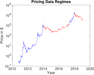
The analysis presented here of the bitcoin price identifies four main epochs. As outlined above the epochs are identified by minimizing the residual between the empirical second-order moments and the modeled power laws, with the modeled power laws having constant parameters within each epoch. The first and the third epochs are similar in terms of persistent dynamics reflecting a strong-herding behavior or confidence in the market trend. This corresponds to a super-diffusive behavior where the log-price changes grow superlinearly in terms of their second moments, so that the price can exhibit relatively larger price swings. Wedged in between these epochs is a period of much less persistence with a relatively low Hurst exponent close to a half correponding essentially to an efficient market behavior. Thus, this does not correspond to a herding behavior with a confidence in the market trend. This mid-epoch starts approximately at the time that the bitcoin exchange Mt. Gox was hacked. We find that in the third epoch, after the confidence in the currency was reestablished, the persistence actually was slightly higher than in the the first epoch of the bitcoin price path. This is an important observation that may explain the price surge. The fourth and final epoch corresponds to a Hurst coefficient of about .4 and thus to an antiherding behavior in an epoch of relative strong price drops. It follows that for the bitcoin price we may think of the Hurst exponent as a market “herding-index”, a measure of a confidence in the market behavior. Epochs of strong herding behavior are characterized by large Hurst exponents (i.e. larger than $1/2$). We remark that the epochs of strong persistence can be associated with relatively strong growth spurs in the price, see Figure 1 below.

The estimation of the Hurst exponent tells us at which level of market confidence we are. It makes it possible to understand if a change in price level and trend signifies a new market regime or if it can be seen as a random local price correction. From the financial viewpoint it is important to observe that the Hurst exponent seems to be a better indicator of market confidence than the volatility which classically is the most important financial parameter. Our story does not stop here with a time-varying market persistence. What is very striking is that the market behaves as if there were an “invisible hand” controlling the variations of the persistence to generate a beautiful effective power law over the entire period of bitcoin existence, see Figure 4 below. Indeed the market is driven and controlled by the market participants so that on any given time epoch there is an effective mean return valid also on the subscales within this period. For the bitcoin market over the total period considered this mean return corresponds to a Hurst exponent of $H=.6$ corresponding to a persistent market and positive correlation of the returns.

Our point of view in this paper is that the main quantity of interest is the second-order correlation structure and what it tells us about market persistence and volatility at different scales and how these concepts are connected. We remark that analysis of high order-moments is theoretically interesting, but becomes very sensitive to tail behavior of returns which limits their practical applicability. By focusing on the second-order temporal correlation structure we can more robustly identify the quantities that are of direct financial interest. Moreover, we show that our multiscale analysis is robust with respect to the marginal distribution of the returns.

Some technical points are discussed in the appendices: In A we give the rigorous model for the multi-fractal process and relate it to our modeling of the observations. The main tool we use to estimate the multi-fractal character of the bitcoin price is the scale spectrum and the associated technique for estimation of the power-law parameters. We present the details of this concept and the estimation procedure in B in a way that can be easily reproduced. As mentioned we use a moving window to track the multi-fractal variations in the price process. One may then wonder whether there is significant residual multi-fractality within the window. In C we introduce a novel notion of a generalized Hurst exponent and a new method to check for within window multi-fractality. Using this method we find that in the epoch just after the Mt. Gox hacking there is significant residual multi-fractality, but otherwise not. One may further wonder whether the fact that the marginal value distribution of the returns associated with the bitcoin price deviates from the Gaussian distribution is important, in particular, whether it could be a source for the observed multi-fractal character. We show in D that this is not the case by using a technique based on a Gaussian transformation. Finally, we comment on a relation to classic chaotic systems in E. We show that indeed the breathtaking growth that the bitcoin cryptocurrency has experienced cannot be well modeled by classic chaotic systems, in fact one has to model in terms of long-range processes of the type considered in this paper.

The outline of the main part of the paper is as follows: In Section 2 we discuss the modeling and estimation procedure that we use for the power law scale spectrum and the results for the bitcoin data. In Section 3 we present the approach for segmentation. We consider measures of scale-based correlations in Section 4 and a measure of multifractality in Section 5. Finally, in Section 6 we conclude.

2 Scale Spectrum of Bitcoin

2.1 Scale Spectrum and Power-law Parameters Estimation

We describe in this section how we compute the scale spectrum and the estimates of the local power-law parameters: the Hurst exponent and the volatility. The details are given in B. The data are the daily bitcoin prices in $ denoted by

$$P(t_{n}),\quad n=1,\ldots,N,$$

where $t_{n}=t_{1}+(n-1)\Delta t$ and $\Delta t$ is the sampling rate (one day). We will consider a window of length $M$, which below will be chosen as one year. We denote the log prices in the $k$th window (with $k\in\{1,\ldots,N-M+1\}$) by

$$\big{(}a_{0}^{(k)}(i)\big{)}_{i=0}^{M-1}=\big{(}\log(P(t_{k+i}))\big{)}_{i=0}^{M-1}.$$ (1)

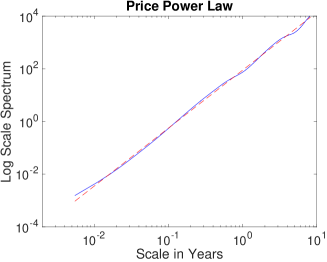
Here the window center time is $\tau_{k}=t_{k}+(M-1)\Delta t/2$. The motivation for this notation is that we view these data as the Haar coefficients at level zero. We next compute the continuous transform Haar wavelet detail coefficients at the different levels $j$ as in (13) and the scale spectral data $S_{j}^{(k)}$ as in (11). We use all available scales apart from the first one so that in (10) we have $j_{\rm i}=2$ and $j_{\rm e}=\lfloor M/2\rfloor$. Thus, we do not use the first scale which is most sensitive to “measurement noise”. Indeed, it is seen from Figure 4 below that the first scale spectral point is slightly enhanced relative to the fitted model.

If the observations come from a fractional Brownian motion with constant Hurst exponent $H$ and volatility $\sigma$ in the way described in A then we have

$$\mathbb{E}\big{[}S_{j}^{(k)}\big{]}=\sigma^{2}h(H)2^{j(2H+1)},$$ (2)

for

$$h(H)=\frac{(1-2^{-2H})}{(2H+2)(2H+1)},$$ (3)

so that

$$\log_{2}\mathbb{E}\big{[}{S}_{j}^{(k)}\big{]}=\log_{2}(\sigma^{2}h(H))+j(2H+1).$$

We can then obtain the estimates of the Hurst exponent $\hat{H}(\tau_{k})$ and the volatility $\hat{\sigma}(\tau_{k})$ by a least squares procedure (linear regression) of $\log_{2}(S_{j}^{(k)})$ as shown in B. We remark that the estimated volatility is the volatility on the $\Delta t$ time scale. The local volatility on the time scale $\tau=m\Delta t$ is $\widehat{\sigma}(\tau_{k})m^{\widehat{H}(\tau_{k})}$.

2.2 Bitcoin Multi-scale Structure

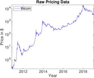
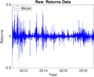
In Figure 1 the left plot shows the daily bitcoin price (in log scale) in $, that is, $P(t_{n}),\quad n=1,\ldots,N$, with $t_{1}$ being November 5th 2010, $t_{N}$ being January 23rd, 2019, and $N=3000$. There is a price observation for every day of the year. The data were obtained from the web site www.coindesk.com/price/bitcoin as daily closing prices. We see that after its introduction the bitcoin experienced a very rapid growth, which was somewhat tamed after about two years. However, the growth stagnated around the beginning of 2014 with the hacking of Mt. Gox exchange until about the beginning of 2017 when a period of strong growth culminated in a maximum price in early 2018. The right plot in Figure 1 shows the returns, that are

$$R_{n}=\frac{P(t_{n})-P(t_{n-1})}{P(t_{n-1})}.$$

From the plot it appears that the volatility was highest in an initial phase and that it has rebounded somewhat in recent years. We examine more closely these qualitative observations by looking at the estimated local power-law parameters next.

Figure 1: The daily raw bitcoin price in log scale (left) and the associated returns, or relative price changes (right).

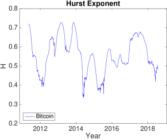
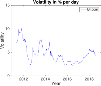
In Figure 2 we show the estimated local Hurst exponent, $\hat{H}(\tau_{k})$, in the left plot and the estimated local volatility, $\hat{\sigma}(\tau_{k})$, in the right plot. These estimates are obtained as described in the previous section with a window width of one year used for computing the local scale spectrum. We see that there are considerable variations in the Hurst exponent. In an early phase of the bitcoin existence both the volatility and the Hurst exponent are high while they decrease after the hacking of Mt. Gox in early 2014. In the last years the Hurst exponent has again increased and it is also seen that the price movements are larger in this period. Note that the time period of minimum price after the hacking event occurs around mid 2015, which is an epoch of relatively small price drift. This epoch corresponds approximately with the minimum Hurst exponent estimate. There is a brief epoch just after the Mt. Gox hacking with the lowest Hurst exponent and thus strong anti-herding behavior, a special event is indeed detected, however its duration is shorter than the window width of one year.

Figure 2: The left plot shows the Hurst exponent as function of the window center time used in the estimation (thus the first data point is half a year after the time of the first price observation with a window width of one year year). The right plot shows the corresponding estimated annual-scale volatility.

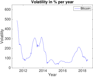
In Figure 3 we show in the right plot the volatility on the annual scale (as in the right plot of Figure 2) and the volatility on the daily scale in the left plot. This illustrates the fact that the variations in the Hurst exponent are the primary driver of annual scale volatility. From the financial perspective it is then clear that variations in the Hurst exponent are of primary importance as they largely drive the annual scale volatility which is the classic measure of risk. In particular it indicates that a volatility estimate based on the mean square of the returns, the empirical quadratic variation, may be strongly biased.

Figure 3: The left plot shows the estimated volatility on the daily scale, the right plot shows the estimated volatility on the annual scale.

Figure 4 shows the global power law, that is the case when the we use all the data shown in Figure 1 to compute the scale spectrum. We can observe a nice power law with effective parameters $H=.6$ and $\sigma=178\%$ on the annual scale.

Figure 4: The global scale spectrum (blue solid line) estimated over the full data set. The estimated parameters are $H=.60$, $\sigma=173\%$. The red dashed straight line is the power law spectrum with the estimated parameters.

We have seen that the spectral characteristics of bitcoin price show temporal variations, moreover, that they aggregate to form a nice power law when observed over the entire period of bitcoin existence. It may then be natural to ask how one best can do a partial aggregation to naturally segment the bitcoin price into sections where the power law is approximately homogeneous within each section and we discuss this in the next section.

3 Segmentation and Regime Switch Detection

Consider a partition of the full data set into $Q$ disjoint segments with width $M_{q}\Delta t$, $q=1,\ldots,Q$ (we have $\sum_{q=1}^{Q}M_{q}=N$). We apply the estimation procedure described in B on each segment. We denote the estimated scale spectrum in each window by $S^{(q)}_{j}$, $j\in\{j_{\rm i}^{(q)},\ldots,j_{\rm e}^{(q)}\}$, where $\{j_{\rm i}^{(q)},\ldots,j_{\rm e}^{(q)}\}$ is the inertial range of interest (we take $j_{\rm i}^{(q)}=2$ and $j_{\rm e}=\lfloor M_{q}/2\rfloor$). We also denote the modeled power-law scale spectrum with the estimated parameters (volatility $\sigma^{(q)}$ and Hurst exponent $H^{(q)}$) by $\overline{S}^{(q)}_{j}$, $j=j_{\rm i}^{(q)},\ldots,j_{\rm e}^{(q)}$ (see (2)). Then we define the total spectral residual by

$$R(M_{1},\ldots,M_{Q})=\sum_{q=1}^{Q}\sum_{j=j_{\rm i}^{(q)}}^{j_{\rm e}^{(q)}}\frac{1}{j}\left(\log_{2}\big{(}S^{(q)}_{j}\big{)}-\log_{2}\big{(}\overline{S}^{(q)}_{j}\big{)}\right)^{2}.$$ (4)

Note that 1) the weighting of the spectral residuals is uniform with respect to the windows, which serves to penalize relatively short windows; 2) the weighting is proportional to the reciprocal scale, $j^{-1}$, which reflects the larger variance of the spectral data for longer scales. Finally we estimate the optimal segmentation by minimizing $R$ with respect to the partitition $(M_{1},\ldots,M_{Q})$ via an exhaustive search (the convexity of the function $R$ is not known).

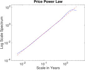
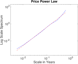
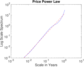
In Figure 5 we show the result of the segmentation procedure when we let $Q=4$ and we implement a two-level search with a coarse grid size of half a year and a fine grid size of five days. The estimated power-law parameters are for the four segments $H=.58,.49,.59,.40$ and $\sigma=225\%,62\%,145\%,62\%$. The first change point (January 16th 2014) corresponds to the hacking of Mt Gox, while the second change point (April 23rd 2017) corresponds to the start phase of the second strong growth period of the bitcoin price approximately at the time it reaches its previous maximum. The final change point (December 5th 2017) corresponds to the initiation of a phase of declining bitcoin price recordings.

Figure 5: The segmentation of the price time series into four epochs. The vertical lines gives the change points in between segments.

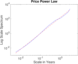
In Figure 6 we show the scale spectra corresponding to the data in the four segments. We remark that using more than four segments does nor lead to a further reduction in the residual $R$. It is remarkable that the local spectra have different power law behaviors and at the same time that the global spectrum has also a power law behavior (Figure 4). The precision of the Hurst estimates can be assessed by the precision obtained with fractional Brownian motion. For the window sizes of the data corresponding to the four windows in Figure 6, this gives a relative standard deviation for the Hurst exponent that is approximately 7% for the two first segments and 10% for the last two shorter segments. Moreover, for the two first segments there is a negligible bias while for the last two segments the bias is approximately $-.03$. The estimator is approximately Gaussian distributed, and thus the first, third, and fourth estimated values for $H$ can be said to be significantly different from $H=1/2$.

Figure 6: The scale spectra in the four estimated epochs (blue solid lines) and the power law spectra with the estimated parameters (red dashed straight lines). The estimated parameters are for the four epochs $H=.58,.49,.59,.40$ and $\sigma=225\%,62\%,145\%,62\%$.

4 Cryptocurrency Multiscale Correlations

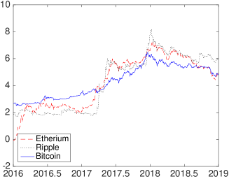
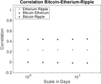
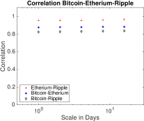
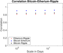
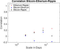
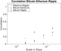
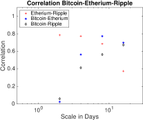
We consider next how the bitcoin price is correlated with some other cryptocurrencies. The two other cryptocurrencies considered are Ethereum and Ripple. We show in Figure 7 the three currencies (daily log-prices) on a common interval of existence, the period January 1st 2016 till December 29th 2018. We consider then the three periods corresponding to 2016, 2017 and 2018 respectively. In the context of the regimes for the bitcoin price estimated in the previous section this corresponds respectively to epochs of (i) relative efficiency and small persistence (ii) strong persistence and a growth spur (iii) strong antipersistence and significant price drop. We compute first the correlation coefficients of the approximation coefficients of the log-price time series, that are the averages of the log-prices over intervals of length $2^{j}$ for $j=0,\ldots,4$. The approximation coefficients give the price level variations at different scales, the dyadic scales between $1$ day and $16$ days. We remark that with one year of daily observations this corresponds to a relative accuracy ranging from roughly 5% till 20%. The case $j=0$ corresponds to the classic measure of correlation of the time series. The results are shown in the top subplots of Figure 8. The first epoch of relative efficiency is associated with smaller cryptocurrency correlation. Moreover, the bitcoin is consistently stronger correlated with Ethereum than with Ripple and the correlations are stable with respect to scale. The bottom subplots show the correlation coefficients of the difference coefficients, that are the $d_{j}$ as in (13) at levels $j=1,\ldots,4$. The case $j=1$ corresponds roughly to daily returns, while the other scales give measures of returns for longer scales. In general the correlation coefficients for the difference coefficients are smaller than for the approximation coefficients and the variability with respect to scale is higher. Indeed the correlation coefficients in the first epoch corresponding to relative efficiency are small. In general there is an enhanced correlation with respect to scale for the correlations between bitcoin and the two other currencies in the strongly persistent or anti-persistent epochs, while there is little observable systematic variation with respect to scale for correlations between Ethereum and Ripple.

Figure 7: Prices of the three cryptocurrencies considered; top (orange) line: bitcoin; middle (blue) line: Ethereum; bottom (red) line: Ripple. The vertical axis is in log scale, but with shifts for the lines to a common mean level.

Figure 8: Top plots show the correlation coefficients of the approximation coefficients in the three years 2016, 2017 and 2018 (left to right), while the bottom plots show the correlation coefficients of the difference coefficients. The (red) crosses are the correlation coefficients between Ethereum and Ripple, the (blue) stars between Ethereum and bitcoin and the (black) diamonds between Ripple and bitcoin.

5 Bitcoin Multifractality

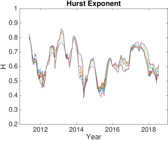
We briefly comment on measure of local multifractality for the bitcoin price and discuss this in more detail in C. We generalize the scale spectrum in (11) to the $q$-moment scale spectrum, $S_{j}(q)$ defined in (26). We can then, as in the above case with $q=2$, estimate the Hurst exponent via linear regression with respect to scale of the log-scale scale spectrum. In the case that the underlying process is fractional Brownian motion and we have a long data set this estimate is independent of $q$ while strong $q$-dependence is a measure of multifractality. We show the result of the Hurst exponent estimate for various values of $q$ in Figure 9. We note that the epoch associated with the Mt. Gox is associated with a particular high degree of multifractality. Thus, this measure identifies the special epoch associated with the hack which not only distinguishes itself via a change in Hurst exponent, but also a brief epoch of deviation from “pure” fractional scaling structure even locally.

Figure 9: Generalized Hurst exponent estimates for $q\in\{1/4,1/2,3/4,1,2,3,4\}$.

6 Conclusions

We have presented a scale-based analysis of the bitcoin cryptocurrency and associated measures of multiscale correlations. The strong growth spurs in the cryptocurrency can be understood in terms of such correlations and “superchaotic” behavior. We have shown that the fractional or anomalous-diffusion behavior that we observe can be attributed to an inherent temporal correlation structure rather than a non-Gaussian marginal character. The analysis is carried out using a Haar wavelet based approach which makes it possible to track local changes in the correlation properties of the price. We find that the changes in the price correlation structure can be used to estimate characteristic epochs of relative structural stationarity in the price evolution. We use the scale spectrum and its parameterization in terms of volatility and Hurst exponent, which we view as a market herding index, as a tool to identify four main epochs for the price evolution. There are two epochs with large Hurst exponents of approximately $.6$, that are characterized by relatively large price moves, and in between there is an epoch with Hurst exponent approximately $.5$, that is characterized by a relatively stable price level. Finally, there is an epoch of relative strong anti-persisitence or negatively correlated returns which corresponds to the recent epoch of price decay. The second epoch of relative efficiency starts after the hacking of the exchange platform Mt. Gox and lasts about $3.5$ years. A main result of our analysis is that over the entire period of bitcoin existence (about seven years) the scale spectrum conforms with that of a homogeneous power law with Hurst exponent about $.6$ which is larger than typical values obtained when considering the equity market [23] or classic currency markets [24].

We have also introduced a measure of multifractality which is indeed relatively strong in the epoch associated with the Mt. Gox hack. We have furthermore introduced a measure of scale-based correlation and have used this to analyze the correlations between Bitcoin and two other cryptocurrencies. We see in particular that the correlations of scale-based returns between bitcoin and Ripple indicate a coherence that increases with scale in inefficient markets.

We remark finally that it is also of interest to look at intraday bitcoin prices. Here we have focused on the spectral characteristics of the daily prices, which are important when the time horizon of interest is on the scale of multiple days. One can expect to have additional high-frequency intraday spectral features which may be somewhat different from those seen for usual currencies and equity markets. We do not consider intraday effects here, but we remark that the data analytic tools set forth in this paper could be used also for considering such intraday spectral features.

Appendix A Modeling Multi-fractional Brownian Motion

The classic model for a random process with power-law behavior is fractional Brownian motion [9], whose increments are stationary and whose power-law parameters, the Hurst exponent and the volatility, are constant. Here we present a class of random processes with local power-law behavior, whose power-law parameters vary in time. This corresponds to a generalization of fractional Brownian motion to multi-fractional Brownian motion. Below we give a precise definition of a multi-fractional Brownian motion and relate it to our model for the observations. Multi-fractional Brownian was introduced in [25, 26] and more details can be found in [27] for instance. Let $H:\mathbb{R}\to(0,1)$ and $\sigma:\mathbb{R}\to(0,\infty)$ be two measurable functions. A real-valued process $B_{H,\sigma}(t)$ is called a multi-fractional Brownian motion with Hurst exponent $H$ and volatility $\sigma$ if it admits the harmonizable representation

$$B_{H,\sigma}(t)=\frac{\sigma_{t}}{\sqrt{C(H_{t})}}{\rm Re}\Big{\{}\int_{\mathbb{R}}\frac{e^{-i\xi t}-1}{|\xi|^{1/2+H_{t}}}d\tilde{W}(\xi)\Big{\}},$$ (5)

where the complex random measure $d\tilde{W}$ is of the form $d\tilde{W}=dW_{1}+idW_{2}$ with $dW_{1},dW_{2}$ two independent real-valued Brownian measures, and $C(h)$ is the normalization function:

$$C(h)=\int_{\mathbb{R}}\frac{4\sin^{2}(\xi/2)}{|\xi|^{1+2h}}d\xi=\frac{\pi}{h\Gamma(2h)\sin(\pi h)}.$$ (6)

Let $h\in(0,1)$ and $s\in(0,\infty)$. If $H_{t}\equiv h$ and $\sigma_{t}\equiv s$, then $B^{(h,s)}(t)\equiv B_{H,\sigma}(t)$ is a fractional Brownian motion with Hurst exponent $h$ and volatility $s$, i.e. a zero-mean Gaussian process with covariance

$$\mathbb{E}\big{[}B^{(h,s)}(t)B^{(h,s)}(t^{\prime})\big{]}=\frac{s^{2}}{2}\big{(}|t|^{2h}+|t^{\prime}|^{2h}-|t-t^{\prime}|^{2h}\big{)}.$$ (7)

Let $\beta\in(0,1)$. Let $H:\mathbb{R}\to(0,1)$ and $\sigma:\mathbb{R}\to(0,\infty)$ be two $\beta$-Hölder functions, such that $\sup_{t}H_{t}<\beta$. The multifractional Brownian motion (5) is a zero-mean continuous Gaussian process that satisfies the Locally Asymptotically Self-Similar property [25]: At any time $\tau\in\mathbb{R}$, we have

$$\lim_{\epsilon\to 0^{+}}{\cal L}\Big{(}\big{(}\frac{B_{H,\sigma}(\tau+\epsilon t)-B_{H,\sigma}(\tau)}{\epsilon^{H_{\tau}}}\big{)}_{t\in\mathbb{R}}\Big{)}={\cal L}\Big{(}\big{(}B^{(H_{\tau},\sigma_{\tau})}(t)\big{)}_{t\in\mathbb{R}}\Big{)},$$ (8)

where ${\cal L}$ means “the distribution of”, which means that there is a fractional Brownian motion with Hurst exponent $H_{\tau}$ and volatility $\sigma_{\tau}$ tangent to the multi-fractional Brownian motion $B_{H,\sigma}$. This implies that its pointwise Hölder regularity is determined by its Hurst exponent.

Here, we shall assume that the parameter functions $H$ and $\sigma$ are smooth with a characteristic time of variation $T_{0}$ so that we can write

$$H_{t}=H_{0}\left(\frac{t}{T_{0}}\right),\quad\sigma_{t}=\sigma_{0}\left(\frac{t}{T_{0}}\right),$$

where $H_{0},\sigma_{0}$ have variations on the order one scale with respect to their dimensionless argument. Recall from Section 2.1 that we assume that we consider the data in a moving window with the $k$th window, $k=1,\ldots,N-M+1$, having center time $\tau_{k}$ and width $M\Delta t$. In the context of the data in (1) we then assume $M\Delta t\ll T_{0}$. In distribution we then model the daily recorded log-price recordings in (1) by

$$a_{0}^{(k)}(i)=\log\left(P(t_{i+k})\right)=\int_{t_{i+k}-\Delta t/2}^{t_{i+k}+\Delta t/2}B^{(h,s)}(t)\,dt,\quad i=0,\ldots,M-1,$$ (9)

with $h=H_{\tau_{k}},s=\sigma_{\tau_{k}}$. That is, the data in (1) are modeled as the level zero approximation coefficients of the process $B^{(h,s)}(t)$ relative to the Haar wavelet basis.

Appendix B Power Law estimation with the Scale Spectrum

We explain the details of how the local power-law parameters are estimated from the log-price data in (1) which are modeled as in (9).

The input parameters are the integers $j_{\rm i}<j_{\rm e}$ that determine the scale range under consideration, the inertial range, and the window size $M$ which is the size of the moving time window in which the local spectra are computed. We must have

$$1\leq j_{\rm i}<j_{\rm e}\leq\lfloor M/2\rfloor.$$ (10)

We proceed as follows:

1. Compute the scale spectrum ${\itbf S}^{(k)}=(S_{j}^{(k)})_{j=j_{\rm i}}^{j_{\rm e}}$ as the local mean square of the wavelet coefficients:

   $$S_{j}^{(k)}=\frac{1}{N_{j}}\sum_{i=0}^{N_{j}-1}\big{(}d_{j}^{(k)}(i)\big{)}^{2},$$ (11)

   where

   $$N_{j} = M-2j+1,$$ (12)

   $$d_{j}^{(k)}(i) = \frac{1}{\sqrt{2j}}\sum_{l=0}^{j-1}a_{0}^{(k)}(l+i)-a_{0}^{(k)}(l+i+j).$$ (13)

2. Define the $(j_{\rm e}-j_{\rm i}+1)$-dimensional vector ${\itbf Y}^{(k)}$ and the $(j_{\rm e}-j_{\rm i}+1)\times 2$-dimensional matrix ${\bf X}$ as

   $${\itbf Y}^{(k)} = \big{(}\log_{2}(S^{(k)}_{j_{\rm i}}),\cdots,\log_{2}(S^{(k)}_{j_{\rm e}})\big{)}^{T},$$ (14)

   $${\bf X} = \left[\begin{array}[]{cc}1&\log_{2}(2j_{\rm i})\\ 1&\log_{2}(2(j_{\rm i}+1))\\ \vdots&\vdots\\ 1&\log_{2}(2j_{\rm e})\end{array}\right],$$ (19)

   and for a $(j_{\rm e}-j_{\rm i}+1)\times(j_{\rm e}-j_{\rm i}+1)$-dimensional weighting matrix ${\bf R}$ compute the regression parameters $\hat{\itbf b}^{(k)}=(\hat{c}^{(k)},\hat{p}^{(k)})^{T}$ defined by

   $$\hat{{\itbf b}}^{(k)}=({\bf X}^{T}{\bf R}^{-1}{\bf X})^{-1}{\bf X}^{T}{\bf R}^{-1}{\itbf Y}^{(k)}.$$ (20)

   In (20) the matrix ${\bf X}$ is the design matrix, ${\bf R}$ is the least squares weighting matrix, and ${\itbf Y}^{(k)}$ is the data vector for the generalized least squares problem that allows to identify the local power-law parameters.

3. Compute the local Hurst exponent and volatility estimates as

   $$\widehat{H}(\tau_{k};{\bf R}) = \frac{\hat{p}^{(k)}-1}{2},$$ (21)

   $$\widehat{\sigma}(\tau_{k};{\bf R}) = \frac{2^{\hat{c}^{(k)}/2}}{\sqrt{h(\widehat{H}(\tau_{k};{\bf R}))}}.$$ (22)

   In (22) the scale-spectral scaling function $h$ is defined by (3).

4. For a diagonal weighting matrix of form (with $q>0$)

   $${R}^{q}_{j_{1}j_{2}} = {j_{1}^{q}}{\bf 1}_{j_{1}}(j_{2}),\quad j_{1},j_{2}\in\{j_{\rm i},\ldots,j_{\rm e}\},$$

   compute

   $$\overline{\bf R}^{(k)}=\begin{array}[t]{c}{\rm argmax}\\ \scriptstyle{{\bf R}\in\{{\bf R}^{1},{\bf R}^{3}\}\displaystyle}\end{array}\left(\widehat{H}(\tau_{k};{\bf R})\right),$$

   and obtain the robust parameter estimates by

   $$\widehat{H}(\tau_{k}) = \widehat{H}(\tau_{k};\overline{\bf R}^{(k)}),$$ (24)

   $$\widehat{\sigma}(\tau_{k}) = \widehat{\sigma}(\tau_{k};\overline{\bf R}^{(k)}).$$ (25)

We remark that in (21) we may threshold the estimation by
$\min(\max(\widehat{H}(\tau_{k};{\bf R}),0.05),0.95)$ in order to avoid any singular behavior. Note also that in order to obtain a robust estimator we have used a combination of two diagonal weighting matrices, see [28] for a discussion of the robustness and precision of this procedure.

Appendix C A Local Measure of Multi-fractality

In [2] the authors use a multi-fractal detrended fluctuation analysis (MF-DFA [3]) to detect multi-fractality. For a given duration $s$, this amounts to divide the time series into equal subsections of duration $s$ and to subtract from the time series a fitted polynomial of order $m$ for each subsection. Then, the variance of the detrended data is computed for each subsection. If the total data length is $N$ then the variances of the detrended data in each subsection are denoted by

$$F^{2}(s,v),\quad v=1,\ldots,N_{s}=\lfloor N/s\rfloor.$$

For a general moment $q>0$ an analogue of the scale spectrum is formed as

$$F_{q}(s)=\left\{\frac{1}{N_{s}}\sum_{v=1}^{N_{s}}F^{2}(s,v)^{q/2}\right\}^{1/q}.$$

A linear regression according to the model

$$\log\left(F_{q}(s)\right)=\log(A)+H(q)\log(s)$$

is carried out to get a generalized Hurst exponent $H(q)$. In the mono-fractal case the generalized Hurst exponent $H(q)$ should be $q$-independent (since $F^{2}(s,v)$ should be independent of $v$) and it should be equal to the actual Hurst exponent. In [2] the authors carry out such an analysis for each of the low and high price epochs (before and after February 2013) for both the bitcoin prices and returns. They find a stronger degree of multi-fractality in the first epoch, as reflected by a stronger dispersion in the generalized Hurst exponent. This is the case for both the returns and prices, moreover, the authors establish (by a randomly shuffling method) that fat-tails are the main source of multi-fractality in both low- and high-price epochs (i.e. before and after February 2013).

Here, we carry out a related analysis with a modified generalized Hurst exponent. First, we want to track the actual multi-fractal character, the changes in the Hurst exponent, that is why we use a moving window rather than a “global” analysis. Second, we want to look at the scaling structure for all scales and therefore do not subtract a fitted trend polynomial.

In order to detect residual multi-fractality within each window we form the generalized scale spectrum by

$$S_{j}{(q)}=\Big{\{}\frac{1}{N_{j}}\sum_{i=0}^{N_{j}-1}|d_{j}(i)|^{q}\Big{\}}^{2/q},$$ (26)

where we suppress the dependence on the window (with center point $\tau_{k}$). When the underlying process is fractional Brownian motion with Hurst exponent $H$ we have (provided $N_{j}\gg 1$ so that $S_{j}{(q)}\approx\mathbb{E}[|d_{j}(1)|^{q}]^{2/q}$):

$$\log_{2}\big{(}S_{j}{(q)}\big{)}\approx\frac{2}{q}\log_{2}\Big{(}\frac{2^{q/2}}{\sqrt{\pi}}\Gamma\big{(}\frac{q+1}{2}\big{)}\Big{)}+\log_{2}(\sigma^{2}h(H))+j(2H+1).$$ (27)

For an arbitrary process we get a generalized Hurst exponent, $H(q)$, via linear regression with respect to this model:

$$\log_{2}\big{(}S_{j}{(q)}\big{)}=\log_{2}(A)+j(2H(q)+1).$$

By (27) this generalized exponent is $q$-independent when the underlying process is mono-fractal Brownian motion.

In Figure 9 we show $H(q;\tau_{k})$ for the bitcoin data as function of window center point $\tau_{k}$. We can see some degree of within window multi-fractality in the first epoch of high Hurst exponent in early 2013, moreover, a rather high degree of within window multi-fractality just after the hacking of Mt. Gox. However, in general the degree of within window multi-fractality is relatively low. We remark that, for a finite window width there is a $q$-dependent bias in the generalized Hurst exponent estimate (as can be shown by a direct calculation for fractional Brownian motion), thus to examine the stability of the multifractal variations and eliminate this bias we center the curves with respect to the mean of the curve with $q=2$.

Appendix D Tail and Marginal Effects

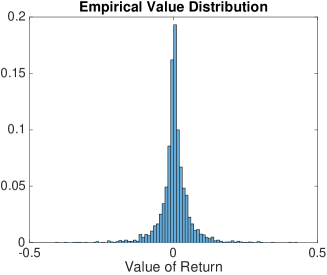
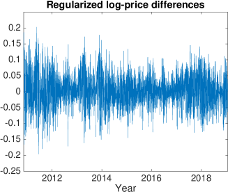
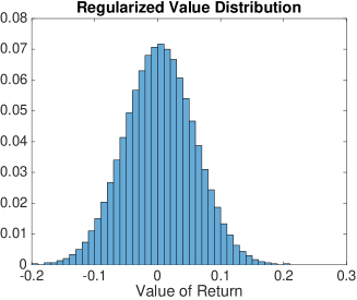
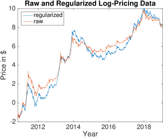
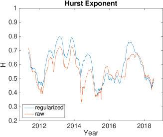
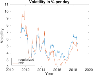
In this appendix we show that the fluctuations in the Hurst exponent, as a measure of multi-fractality, are not due to tail or marginal non-Gaussianity effects. The raw log-price differences are shown in Figure 10. The histogram exhibits a heavy-tail distribution. We regularize by a Gaussian marginal transformation of the log-price differences. Note that the log prices are differentiated, then the transformation is carried out (see Figure 11), and the regularized log-prices created by integration (see Figure 12) and subsequently used in the multi-scale analysis as before. We can see in Figure 13 that the power-law parameters are essentially the same ones for the raw data and for the regularized (Gaussianized) data. The only minor change is that the procedure applied to the regularized data seems to slightly overestimate large $H$ values compared to the case where the raw data are processed directly. Other regularization methods (such as truncation at plus or minus two standard deviations) give the same result.

Figure 10: Log-price differences (left) over the entire period of bitcoin existence and histogram (right).

Figure 11: Regularized log-price differences (left) over the entire period of bitcoin existence and histogram (right).

Figure 12: Raw (red) and regularized (blue) log prices.

Figure 13: Hurst exponent (left) and daily volatility (right) of the raw returns (red) and the regularized returns (blue).

Appendix E On Chaotic Behavior

Following [2] we can in the simplest case of a linear homogeneous system of embedding dimension one consider a chaotic system by

$$X_{n+1}=aX_{n}+\sigma\epsilon_{n},\quad X_{0}=x_{0},$$

with $\epsilon_{n}$ a sequence of independent and identically distributed standard Gaussian noise terms. The associated Lyapunov exponent is $\lambda=\log(a)$. If $\lambda>0$ then we have a chaotic system and an exponential growth:

$${\rm St.Dev}\left[X_{n}\right]=\sigma\sqrt{\frac{e^{2\lambda n}-1}{e^{2\lambda}-1}}.$$

Above we found from the global spectrum, see Figure 4, that the effective returns in the Gaussian case could be modeled as increments of fractional Brownian motion with Hurst exponent $H=.6$. In the continuous limit we may then model the price process by

$$P(n\Delta t)=p_{0}\exp\big{(}\sigma B^{H}(n\Delta t)\big{)},$$

and we have

$${\rm St.Dev}\left[P(n\Delta t)\right]=p_{0}\exp\big{(}\sigma^{2}|n\Delta t|^{2H}\big{)}\Big{(}1-\exp\big{(}-\sigma^{2}|n\Delta t|^{2H}\big{)}\Big{)}^{1/2}.$$

Thus, the price process, with $H=.6$, grows at super-exponential rate or is “super-chaotic”. In the anti-persistent case with $H<1/2$ the price process grows at sub-exponential rate. Note also that the return process itself is fractional Gaussian noise, and thus exhibits long-range correlations, however, is stationary and does not exhibit a chaotic behavior.

References

- [1] S. Nakamoto, Bitcoin: A peer-to-peer electronic cash system, https://bitcoin.org/en/bitcoin-paper (2008).
- [2] S. Lahmiria, S. Bekiros, Chaos, randomness and multi-fractality in bitcoin market, Chaos, Solitons and Fractals 106 (2018) 28–34.
- [3] J. W. Kantelhardt, S. A. Zschiegner, E. Koscielny-Bunde, S. Havlind, A. Bunde, H. E. Stanley, Multifractal detrended fluctuation analysis of nonstationary time series, Physica A 316 (2002) 87–114.
- [4] G. Gajardoa, W. Kristjanpollera, M. Minutolob, Does bitcoin exhibit the same asymmetric multifractal cross-correlations with crude oil, gold and djia as the euro, great british pound and yen?, Chaos, Solitons and Fractals 109 (2018) 195–205.
- [5] A. F. Bariviera, M. J. Basgall, W. Hasperue, M. Naiouf, Some stylized facts of the bitcoin market, Physica A 484 (2017) 82–90.
- [6] J. Alvarez-Ramirez, J. E. Rodriguez, C. Ibarra-Valdez, Long-range correlations and asymmetry in the bitcoin market, Physica A 492 (2018) 948–955.
- [7] S. Begušić, Z. Kostanjčar, H. Stanley, B. Podobnik, Scaling properties of extreme price fluctuations in bitcoin markets, Physica A 510 (2018) 400–406.
- [8] J.-P. Fouque, G. Papanicolaou, K. R. Sircar, K. Sølna, Multiscale Stochastic Volatility for Equity, Interest Rate, and Credit Derivatives, Springer, 2011.
- [9] B. B. Mandelbrot, J. Van Ness, Fractional brownian motion, fractional noises and applications, SIAM Review 10 (1968) 422–437.
- [10] B. B. Mandelbrot, When can price be arbitraged efficiently? A limit to the validity of the random walk and martingale models, Rev. Econom. Statis 53 (1971) 225–236.
- [11] B. B. Mandelbrot, Fractals and Scaling in Finance. Discontinuity, Concentration, Risk, Springer, New York, 1997.
- [12] E. Bayraktar, H. V. Poor, K. R. Sircar, Estimating the fractal dimension of the s&p 500 index using wavelet analysis,, International Journal of Theoretical and Applied Finance 7 (2004) 615–643.
- [13] G. Gajardo, W. Kristjanpoller, Asymmetric multifractal cross-correlations and time varying features between latin-american stock market indices and crude oil market, Chaos, Solitons and Fractals (2017) 121–128.
- [14] G. Oh, C. Eom, S. Havlin, W. S. Jung, F. Wang, H. E. Stanley, S. Kim, A multifractal analysis of Asian foreign exchange markets, Eur. Phys. J. B 85 (2012) 214.
- [15] D. O. Cajueiroa, B. M. Tabak, The hurst exponent over time: testing the assertion that emerging markets are becoming more efficient, Physica A 336 (2004) 521–537.
- [16] J. Alvarez-Ramirez, M. Cisneros, C. Ibarra-Valdez, A. Soriano, Multifractal Hurst analysis of crude oil prices, Physica A 313 (2002) 651–670.
- [17] J. Elder, A. Serletis, Long memory in energy futures prices, Review of Financial Economics 17 (2008) 146–155.
- [18] Z.-Q. Jiang, W.-J. Xie, W.-X. Zhou, Testing the weak-form efficiency of the WTI crude oil futures market, Physica A 405 (2014) 235–244.
- [19] N. Kalamaras, K. Philippopoulos, D. Deligiorgi, C. G. Tzanis, G. Karvounis, Multifractal scaling properties of daily air temperature time series, Chaos, Solitons and Fractals (2017) 38–43.
- [20] M. Laib, J. Golay, L. Telesca, M. Kanevski, Multifractal analysis of the time series of daily means of wind speed in complex regions, Chaos, Solitons and Fractals (2018) 118–127.
- [21] G. Papanicolaou, K. Sølna, Wavelet based estimation of local Kolmogorov turbulence, in: Long-Range Dependence Theory and Applications, Birkhäuser, Boston, 2001, pp. 473–506.
- [22] M. Rajkovic, M. Skoric, K. Sølna, G. Antar, Characterization of local turbulence in magnetic confinement devices, Nucl. Fusion 48 (2008) 024016.
- [23] C. Eom, S. Choi, G. Oh, W.-S. Jung, Hurst exponent and prediction based on weak-form efficient market hypothesis of stock markets, Physica A 387 (2008) 4630–4636.
- [24] J. Yao, C. L. Tan, A case study on using neural networks to perform technical forecasting of forex, Neurocomputing 34 (2000) 79–98.
- [25] A. Benassi, S. Jaffard, D. Roux, Gaussian processes and pseudodifferential elliptic operators, Revista Mathematica Iberoamericana 13 (1997) 19–90.
- [26] R. F. Peltier, J. Lévy-Vehel, Multifractional brownian motion: definition and preliminary results, Tech. Rep. 2645, INRIA (August 1995).
- [27] S. Cohen, J. Istas, Fractional Fields and Applications, Springer, Berlin, 2013.
- [28] J. Garnier, K. Sølna, Emergence of turbulent epochs in oil prices, http://arxiv.org/abs/1808.09382.