$O(N)$ Hierarchical algorithm for computing the expectations of truncated multi-variate normal distributions in $N$ dimensions

Abstract

In this paper, we study the $N$-dimensional integral $\phi(\mathbf{a},\mathbf{b};A)=\int_{\mathbf{a}}^{\mathbf{b}}H(\mathbf{x})f(\mathbf{x}|A)\text{d}\mathbf{x}$ representing the expectation of a function $H(\mathbf{X})$ where $f(\mathbf{x}|A)$ is the truncated multi-variate normal (TMVN) distribution with zero mean, $\mathbf{x}$ is the vector of integration variables for the $N$-dimensional random vector $\mathbf{X}$, $A$ is the inverse of the covariance matrix $\Sigma$, and $\mathbf{a}$ and $\mathbf{b}$ are constant vectors. We present a new hierarchical algorithm which can evaluate $\phi(\mathbf{a},\mathbf{b};A)$ using asymptotically optimal $O(N)$ operations when $A$ has “low-rank” blocks with “low-dimensional” features and $H(\mathbf{x})$ is “low-rank”. We demonstrate the divide-and-conquer idea when $A$ is a symmetric positive definite tridiagonal matrix, and present the necessary building blocks and rigorous potential theory based algorithm analysis when $A$ is given by the exponential covariance model. Numerical results are presented to demonstrate the algorithm accuracy and efficiency for these two cases. We also briefly discuss how the algorithm can be generalized to a wider class of covariance models and its limitations.

03D20, 34B27, 62H10, 65C60, 65D30, 65T40

1 Introduction

In this paper, we study the efficient computation of the expectation of function $H(\mathbf{X})$ given by

(1) $$\phi(\mathbf{a},\mathbf{b};A) = \int_{\mathbf{a}}^{\mathbf{b}}H(\mathbf{x})f(\mathbf{x}|A)\text{d}\mathbf{x}$$

$$= \int_{a_{1}}^{b_{1}}\cdots\int_{a_{N}}^{b_{N}}H(\mathbf{x})|\Sigma|^{-1/2}(2\pi)^{-N/2}e^{-\frac{1}{2}\mathbf{x}^{T}A\mathbf{x}}\text{d}x_{N}\cdots\text{d}x_{1},$$

where the $N$-dimensional random vector $\mathbf{X}=(X_{1},\ldots,X_{N})^{T}$ follows the truncated multivariate normal distribution (TMVN), $f(\mathbf{x}|A)$ is the $N$-dimensional multivariate Gaussian probability density function with zero mean and covariance matrix $\Sigma$, $A$ is the inverse of the symmetric positive definite (SPD) $N\times N$ covariance matrix $\Sigma$, $\mathbf{x}$ is the integration variable, and the integration limits are $\mathbf{a}=(a_{1},\ldots,a_{N})^{T}$ and $\mathbf{b}=(b_{1},\ldots,b_{N})^{T}$ which form a hyper-rectangle in $\mathbb{R}^{N}$. The efficient computation of $\phi$ is very important for many applications, including those in spatial and temporal statistics and in the study of other high dimensional random data sets where the Gaussian distribution is commonly used, see [3, 4, 5, 6, 10, 13, 16, 17, 43] and references therein. Note that $|\Sigma|^{-1/2}(2\pi)^{-N/2}$ is a constant. When $\Sigma$ has low-rank properties, $|\Sigma|^{-1/2}$ can be evaluated efficiently using existing low-rank linear algebra techniques [23, 27, 29, 31]. we ignore this term to simplify our discussions in this paper.

Due to the “curse of dimensionality”, direct evaluation of the $N$-dimensional integral using standard quadrature rules is computationally demanding (and impossible for many settings using today’s supercomputers), and most existing schemes either scale poorly when the dimension $N$ increases or rely on the Monte Carlo methods for very high dimensional cases [8, 12, 18, 19, 20, 22, 35, 30, 37, 38, 40, 41]. A good review of existing techniques can be found in [19]. The purpose of this paper is to show that when there exist special structures in $H$ and $A$ (or equivalently in $\Sigma$), fast direct evaluation of the $N$-dimensional integral becomes possible. In particular, when the function $H(\mathbf{x})$ is “low-rank” and the matrix $A$ has hierarchical low-rank blocks with “low-dimensional” singular vectors in their singular value decompositions, asymptotically optimal $O(N)$ hierarchical algorithms can be developed, by compressing these compact features and efficiently processing them “locally” on a hierarchical tree structure. We leave the mathematical rigorous definitions of the “low-rank” and “low-dimensional” concepts to later discussions, but only mention that such “compact” structures exist in many important applications. For example, when the high dimensional data can be properly clustered, e.g., by using their spatial or temporal locations and relative distance or pseudo-distance, the matrix blocks describing the “interactions” between different clusters are often low-rank as revealed by the principal component analysis (PCA).

This paper presents the algorithm analysis and implementation details for two representative matrices: (a) when $A$ is a tridiagonal SPD matrix; and (b) when $A$ has the same form as the covariance matrix in the exponential covariance model in one dimensional setting. In case (b) when $A$ is the exponential covariance matrix, the original covariance matrix $\Sigma=A^{-1}$ is approximately a tridiagonal system. In the numerical algorithm for both cases, a downward pass is first performed on a hierarchical tree structure, by introducing a $t$-variable to divide the parent problem (involving a function with no more than $2$ “effective” variables) into two child problems, each involving a function with no more than $2$ “effective” variables. The relation coefficients between the parent’s effective variables, new $t$-variable, and children’s effective variables are computed and stored for each tree node. At the leaf level, the one dimensional integral which only involves one $x_{j}$ variable is evaluated either analytically or numerically, and then approximated numerically by a global Fourier series representation. An upward pass is then performed, to recursively forming the approximating Fourier series of the parent’s $2$-effective variable function using those from its two children. The function value $\phi$ in Eq. (1) is simply given by the constant function (with two “null variables”) at the root level of the tree structure. The presented hierarchical algorithms share many similar features as many existing fast hierarchical algorithms in scientific computing, including the classical fast Fourier transform (FFT) [11], multigrid method (MG) [9, 28], fast multipole method (FMM) [25, 26], and the fast direct solvers (FDS) and hierarchical matrix ($\mathcal{H}$-matrix) algorithms [23, 31, 27, 29].

This paper is organized as follows. In Sec. 2, we introduce the mathematical definitions of the “low-rank” and “low-dimensional” concepts. In Sec. 3, we present the details of a hierarchical algorithm for computing $\phi$ when $A$ is a tridiagonal matrix. In Sec. 4, we show how the algorithm can be generalized to the case when $A$ has the same form as the exponential covariance matrix in one dimensional setting, and present the rigorous analysis using potential theory from ordinary and partial differential equation analysis, as the exponential covariance model in one dimension is closely related with the Green’s function and integral equation solutions of the boundary value ordinary differential equation $u(x)-u^{\prime\prime}(x)=f(x)$. Numerical results are presented to demonstrate the accuracy, stability, and $O(N)$ complexity of the new hierarchical algorithm for both cases. In Sec. 5, we discuss how the algorithm can be generalized to more complicated cases as well as its limitations. In particular, our current algorithm implementation relies heavily on existing numerical tools and software packages for accurately processing multi-variable functions (e.g., high dimensional non-uniform FFT or sparse grid techniques). Many of these tools are unfortunately still unavailable even when the number of independent variables is approximately $5\sim 20$. Finally in Sec. 6, we summarize our results.

2 Low-rank and Low-dimensional Properties

Our algorithm can be applied to a function $H(\mathbf{x})$ with the following structure,

(2) $$H(\mathbf{x})=\sum_{p=1}^{P}u_{p,1}(x_{1})u_{p,2}(x_{2})\cdots u_{p,N}(x_{N})=\sum_{p=1}^{P}\prod_{k=1}^{N}u_{p,k}(x_{k}),$$

where $P$ is assumed to be a small constant independent of $N$, and each function $u_{p,k}$ is a single variable function, not necessarily a continuous function. As the separation of variables

$$H(x,y)=\sum_{p=1}^{P}u_{p}(x)v_{p}(y)$$

can be considered as the non-orthogonalized function version of the singular value matrix decomposition

$$H_{m\times n}=U_{m\times P}\Lambda_{P\times P}V^{T}_{P\times n},$$

we refer to a function $H$ with a representation in Eq. (2) as a low-rank (rank-$P$) function. Plugging Eq. (2) into Eq. (1), the original problem of evaluating $\phi$ now becomes the evaluations of $P$ integrals, each has the form

(3) $$\phi_{p}(\mathbf{a},\mathbf{b};A)=\int_{a_{1}}^{b_{1}}\cdots\int_{a_{N}}^{b_{N}}\prod_{k=1}^{N}u_{p,k}(x_{k})\exp\left(-\frac{1}{2}\mathbf{x}^{T}A\mathbf{x}\right)\text{d}x_{N}\cdots\text{d}x_{1}.$$

We focus on $\phi_{p}$ in the following discussions, and simply denote $\phi_{p}$ as $\phi$.

For the inverse $A$ of the covariance matrix $\Sigma$, we assume it belongs to a class of hierarchical matrices ($\mathcal{H}$-matrices) [27, 29] with low-rank off-diagonal blocks. A sample Hierarchical matrix after $2$ (left) and $3$ (right) divisions is demonstrated in Fig. 1, where the blue square block represents the self-correlation within each cluster of random variables $X_{i}$, and the green block shows the correlation between two different clusters. We define a cluster in the original domain as a set of indices of the column vectors, and a cluster in the target space as a set of indices of the row vectors. The correlation between the cluster $J$ of the original domain and cluster $K$ of the target space is described by the matrix block formed by only extracting the $K$-entries from the $J$-columns. We consider $\mathcal{H}$-matrices with low-rank off-diagonal blocks, by assuming that the ranks of all the off-diagonal blocks are bounded by a constant $P$, which is independent of the block matrix size. We use $P$ to represents the dimension of a subspace or the rank of a matrix in this paper, and the rank $P$ of the off-diagonal blocks can be different from the rank $P$ in Eq. (2). In numerical linear algebra, “low-rank off-diagonal block” means that the off-diagonal block $A_{i,j}$ of size $n\times n$ has the following singular value decomposition

$$A_{i,j}=U_{i,j}\Lambda_{i,j}V^{T}_{i,j},$$

where $U$ and $V$ are of size $n\times P$ and respectively contain the orthonormal vectors in the target space and original domain, and $\Lambda$ is a size $P\times P$ diagonal matrix with ordered and non-negative diagonal entries. As the random variables $\{X_{i},i=1,\ldots,N\}$ are clustered hierarchically, we index the block matrices $A_{i,j}$ differently from those commonly used in matrix theory to emphasize this hierarchical structure in the $\mathcal{H}$-matrix, where $i$ represents the level of the matrix block, and $j$ is its index in that particular level. The original matrix $A$ is defined as the level $0$ matrix. After the $1^{st}$ division, the $4$ matrix blocks are indexed $(1,1)$, $(1,2)$, $(1,3)$, and $(1,4)$. The diagonal matrix blocks will be further divided and the off-diagonal matrices become leaf nodes to form an adaptive quad-tree structure. In the left of Fig. 1, the matrix $A_{1,2}$ denotes the second matrix block at level $1$, representing the correlations between the second cluster in the original domain and first cluster in the target space. For the covariance matrix, as the target space and original domain are the one and the same, the indices of the random variables $\mathbf{X}$ (and integration variables $\mathbf{x}$) will be used to cluster the indices of both the target space and original domain, to form a uniform binary tree structure. In the following, we focus on the integration variables $\{x_{i},i=1,\ldots,N\}$, which are referred to as the $x$-variables.

Figure 1: $\mathcal{H}$-matrix after $2$ (left) and $3$ (right) divisions, with low-rank off-diagonal blocks (green).

Next, we consider the “low-dimensional” concept, by studying a function with $M$ $t$-variables $t_{1}$, $t_{2}$, $\ldots$, $t_{M}$ of the form

$$F(t_{1}\mathbf{u}_{1}+t_{2}\mathbf{u}_{2}+\cdots+t_{M}\mathbf{u}_{M}).$$

When the dimension $P$ of the vector space $span\{\mathbf{u}_{1},\mathbf{u}_{2},\ldots,\mathbf{u}_{M}\}$ is much less than $M$, $P<<M$, we say $F$ is a “low-dimensional” function. Assuming the basis for the vector space $span\{\mathbf{u}_{1},\mathbf{u}_{2},\ldots,\mathbf{u}_{M}\}$ is given by $\{\mathbf{v}_{1},\mathbf{v}_{2},\ldots,\mathbf{v}_{P}\}$, the function $F$ can be considered as an “effective” $M$ variable function, where the new $w$-variables $\{w_{1},w_{2},\ldots,w_{P}\}$ are combinations of the $t$-variables and satisfy the relation

$$w_{1}\mathbf{v}_{1}+w_{2}\mathbf{v}_{2}+\cdots+w_{P}\mathbf{v}_{P}=t_{1}\mathbf{u}_{1}+t_{2}\mathbf{u}_{2}+\cdots+t_{M}\mathbf{u}_{M}.$$

The low-rank and low-dimensional structures exist in many practical systems. The well studied low-rank concept measures the rank of a matrix block and is closely related with the principal component analysis in statistics and singular value decomposition (SVD) in numerical linear algebra. When the data can be clustered, the covariance matrix block describing the relations between two different clusters is often low-rank, and both the storage of such a matrix block and related operations can be reduced significantly using today’s low-rank linear algebra techniques. The low-dimensional property in this paper considers the special structures in the singular vectors of the SVD decomposition of the low-rank off-diagonal blocks. Consider two clusters of the $x$-variables and the space formed by extracting all the corresponding sub-vectors describing the relations of these two clusters from the singular vectors in the SVD decompositions of all the off-diagonal matrices. When the covariance matrix is defined by a covariance function using the spatial or temporal locations (or pseudo-locations) $z_{i}$ and $z_{j}$ of the corresponding random variables $X_{i}$ and $X_{j}$, the covariance function is often “smooth” and only contains “low-frequency” information when $i\neq j$, it can be well approximated by a few terms of truncated Taylor expansion (or other basis functions) when a separation of variables is performed on the covariance function determined by the two location variables $z_{i}$ and $z_{j}$. In this case, all the singular vectors are the discretized versions of the polynomial basis functions at locations corresponding to the cluster index sets. The dimension of the space formed by these singular vectors is therefore determined by the highest degree of the polynomial basis functions. When the $\mathbf{u}_{i}$ vectors are extracted from these singular vectors, the function $F(t_{1}\mathbf{u}_{1}+t_{2}\mathbf{u}_{2}+\cdots+t_{M}\mathbf{u}_{M})$ will be low-dimensional and the number of effective variables is also determined by the highest degree of the polynomial basis functions. The special structures in the singular vectors were also used in [31, 32, 33]. The low-rank and low-dimensional concepts will be further studied in the next two sections.

3 Case I: Tridiagonal System

We demonstrate the basic ideas of the hierarchical algorithm by studying a simple tridiagonal system

(4) $$A=\left[\begin{array}[]{rrrrrrr}4&-2&0&.&.&.&0\\ -2&4&-2&0&.&.&0\\ 0&-2&4&-2&0&.&0\\ .&.&.&.&.&.&.\\ .&.&.&.&.&.&.\\ .&.&.&.&.&.&.\\ 0&.&.&.&0&-2&4\end{array}\right]_{N\times N}.$$

We assume $N=2^{L}$ and first consider a constant function $H(\mathbf{x})$ to simplify the notations and discussions. The algorithm for more general low-rank $H(\mathbf{x})$ in Eq. (3) only requires a slight change in the code for the leaf nodes, which will become clear after we present the algorithm details for the simplified integration problem

(5) $$\phi(\mathbf{a},\mathbf{b};A) = \int_{a_{1}}^{b_{1}}\cdots\int_{a_{N}}^{b_{N}}e^{-\frac{1}{2}\mathbf{x}^{T}A\mathbf{x}}\text{d}x_{N}\cdots\text{d}x_{1}$$

$$= \int_{\mathbf{a}}^{\mathbf{b}}e^{\left(-2x_{1}^{2}+2x_{1}x_{2}-2x_{2}^{2}+\cdots-2x_{k}^{2}+{\color[rgb]{1,0,0}2x_{k}x_{k+1}}-2x_{k+1}^{2}+\cdots-2x_{N-1}^{2}+2x_{N-1}x_{N}-2x_{N}^{2}\right)}\text{d}\mathbf{x},$$

where $k=2^{L-1}=N/2$. The tridiagonal matrix is a very special $\mathcal{H}$-matrix, where each off-diagonal matrix block only contains one non-zero number either at the lower-left or upper-right corner of the matrix block and is rank $1$. The singular vectors are either $\mathbf{u}_{i}=[1,0,0,\ldots,0]^{T}$ or $\mathbf{u}_{i}=[0,0,\ldots,0,1]^{T}$. For any given cluster of indices, the number of effective variables in $t_{1}\mathbf{u}_{1}+t_{2}\mathbf{u}_{2}+\cdots+t_{M}\mathbf{u}_{M}$ is therefore no more than 2, and the only non-zero numbers are located either at the first or the last entry in the singular vectors $\mathbf{u}_{1}$, $\mathbf{u}_{2}$, $\ldots$, $\mathbf{u}_{M}$.

3.1 Divide and Conquer on a Hierarchical Tree

Note that the $x$-variables $[x_{1},\ldots,x_{k}]$ and $[x_{k+1},\ldots,x_{N}]$ are coupled in the integrand only through one term $2x_{k}x_{k+1}$. If this “weak coupling” term had not been there, then we would have two completely decoupled “child problems”, and the integral could be evaluated as

$$\begin{array}[]{l}\int_{\mathbf{a}}^{\mathbf{b}}e^{\left(-2x_{1}^{2}+2x_{1}x_{2}-2x_{2}^{2}+\cdots-2x_{k}^{2}-2x_{k+1}^{2}+\cdots-2x_{N-1}^{2}+2x_{N-1}x_{N}-2x_{N}^{2}\right)}\text{d}\mathbf{x}\\ =\left(\int_{a_{1}}^{b_{1}}\cdots\int_{a_{k}}^{b_{k}}e^{\left(-2x_{1}^{2}+2x_{1}x_{2}-2x_{2}^{2}+\cdots-2x_{k}^{2}\right)}\text{d}x_{k}\cdots\text{d}x_{1}\right)\cdot\\ \left(\int_{a_{k+1}}^{b_{k+1}}\cdots\int_{a_{N}}^{b_{N}}e^{\left(-2x_{k+1}^{2}+\cdots-2x_{N-1}^{2}+2x_{N-1}x_{N}-2x_{N}^{2}\right)}\text{d}x_{N}\cdots\text{d}x_{k+1}\right).\end{array}$$

If the same assumptions could be made to each “child problem”, then the high-dimensional integral would become the product of $N$ one-dimensional integrals.

A convenient tool to decouple the $x$-variables in order to have two child problems is to use the Fourier transform formula for the Gaussian distribution as

(6) $$e^{-(x-y)^{2}}=c\int_{-\infty}^{\infty}e^{2it(x-y)}e^{-t^{2}}\text{d}t=c\int_{-\infty}^{\infty}{\color[rgb]{1,0,0}e^{2itx}e^{-2ity}}e^{-t^{2}}\text{d}t$$

where $i=\sqrt{-1}$ and $c=\frac{1}{\sqrt{\pi}}$. Note that the variables $x$ and $y$ are decoupled on the right hand side. Completing the square in Eq. (5) and applying the formula in Eq. (6) to the resulting $(x_{k}-x_{k+1})^{2}$ term (in red) in the integral, we get

$$\begin{array}[]{l}\phi(\mathbf{a},\mathbf{b};A)=\int_{\mathbf{a}}^{\mathbf{b}}e^{\left(-2x_{1}^{2}+2x_{1}x_{2}-2x_{2}^{2}+\cdots{\color[rgb]{0,0,1}-2x_{k}^{2}+2x_{k}x_{k+1}-2x_{k+1}^{2}}+\cdots-2x_{N-1}^{2}+2x_{N-1}x_{N}-2x_{N}^{2}\right)}\text{d}\mathbf{x}\\ =\int_{\mathbf{a}}^{\mathbf{b}}e^{\left(-2x_{1}^{2}+2x_{1}x_{2}-2x_{2}^{2}+\cdots{\color[rgb]{0,0,1}-x_{k}^{2}{\color[rgb]{1,0,0}-(x_{k}-x_{k+1})^{2}}-x_{k+1}^{2}}+\cdots-2x_{N-1}^{2}+2x_{N-1}x_{N}-2x_{N}^{2}\right)}\text{d}\mathbf{x}\\ =c\int_{-\infty}^{\infty}e^{-t^{2}}h_{1,1}(t)h_{1,2}(t)\text{d}t\end{array}$$

where $h_{1,1}(t)$ and $h_{1,2}(t)$ are both single $t$-variable functions given by

$$\begin{array}[]{l}h_{1,1}(t)=\int_{a_{1}}^{b_{1}}\cdots\int_{a_{k}}^{b_{k}}e^{\left(-2x_{1}^{2}+2x_{1}x_{2}-2x_{2}^{2}+\cdots{\color[rgb]{0,0,1}-x_{k}^{2}+2ix_{k}t}\right)}\text{d}x_{k}\cdots\text{d}x_{1},\\ h_{1,2}(t)=\int_{a_{k+1}}^{b_{k+1}}\cdots\int_{a_{N}}^{b_{N}}e^{\left({\color[rgb]{0,0,1}-2ix_{k+1}t-x_{k+1}^{2}}+\cdots-2x_{N-1}^{2}+2x_{N-1}x_{N}-2x_{N}^{2}\right)}\text{d}x_{N}\cdots\text{d}x_{k+1}.\end{array}$$

Note that the $x$-variables in the original problem (associated with a root node at level $0$ of a binary tree structure) are divided into two subsets of the same size, each set is associated with a “child node” and a single $t$-variable function $h_{1,k}(t)$, $k=1$ or $k=2$.

By introducing two new $t$-variables $t_{1,1}$ and $t_{1,2}$ for the functions $h_{1,1}$ and $h_{1,2}$, respectively, the same technique can be applied to decouple the $x$-variables $[x_{1},\ldots,x_{\frac{k}{2}}]$ and $[x_{\frac{k}{2}+1},\ldots,x_{k}]$ in $h_{1,1}(t)$ and the $x$-variables $[x_{k+1},\ldots,x_{\frac{3k}{2}}]$ and $[x_{\frac{3k}{2}+1},\ldots,x_{N}]$ in $h_{1,2}(t)$, to derive

$$h_{1,1}(t)=c\int_{-\infty}^{\infty}e^{-t_{1,1}^{2}}h_{2,1}(t_{1,1})h_{2,2}(t_{1,1},t)\text{d}t_{1,1}$$

$$h_{1,2}(t)=c\int_{-\infty}^{\infty}e^{-t_{1,2}^{2}}h_{2,3}(t,t_{1,2})h_{2,4}(t_{1,2})\text{d}t_{1,2},$$

where

$$\begin{array}[]{l}h_{2,1}(t_{1,1})=c\int_{a_{1}}^{b_{1}}\cdots\int_{a_{\frac{k}{2}}}^{b_{\frac{k}{2}}}e^{\left(-2x_{1}^{2}+2x_{1}x_{2}-2x_{2}^{2}+\cdots{-x_{\frac{k}{2}}^{2}+2ix_{\frac{k}{2}}t_{1,1}}\right)}\text{d}x_{\frac{k}{2}}\cdots\text{d}x_{1},\\ h_{2,2}(t_{1,1},t)=c\int_{a_{\frac{k}{2}+1}}^{b_{\frac{k}{2}+1}}\cdots\int_{a_{k}}^{b_{k}}e^{\left(-2ix_{\frac{k}{2}+1}t_{1,1}-x_{\frac{k}{2}+1}^{2}+\cdots-x_{k}^{2}+2ix_{k}t\right)}\text{d}x_{k}\cdots\text{d}x_{\frac{k}{2}+1},\\ h_{2,3}(t,t_{1,2})=c\int_{a_{k+1}}^{b_{k+1}}\cdots\int_{a_{\frac{3k}{2}}}^{b_{\frac{3k}{2}}}e^{\left(-2ix_{k+1}t-x_{k+1}^{2}+\cdots-x_{\frac{3k}{2}}^{2}+2ix_{\frac{3k}{2}}t_{1,2}\right)}\text{d}x_{\frac{3k}{2}}\cdots\text{d}x_{k+1},\\ h_{2,4}(t_{1,2})=c\int_{a_{\frac{3k}{2}+1}}^{b_{\frac{3k}{2}+1}}\cdots\int_{a_{N}}^{b_{N}}e^{\left({-2ix_{\frac{3k}{2}+1}t_{1,2}-x_{\frac{3k}{2}+1}^{2}}+\cdots+2x_{N-1}x_{N}-2x_{N}^{2}\right)}\text{d}x_{N}\cdots\text{d}x_{\frac{3k}{2}+1},\end{array}$$

Repeating this procedure recursively on the hierarchical tree structure derived by recursively dividing the parent’s $x$-variable set into two child subsets of the same size, a hierarchical $h$-function $h_{l,k}$ will be defined for each tree node, where $\{l,k\}$ is the index of the tree node defined in the same way as that of the $x$-variable sets. One can show that for a parent node with index $p$, its $h$-function $h_{p}(t_{l},t_{r})$ (with at most two $t$-variables $t_{l}$ and $t_{r}$) can be computed from the two child functions $h_{c_{1}}(t_{l},t_{m})$ and $h_{c_{2}}(t_{m},t_{r})$ (each with at most two $t$-variables) by integrating the $t$-variable $t_{m}$ used to decouple the parent problem using Eq. (6) as

(7) $${h_{p}(t_{l},t_{r})=c\int_{-\infty}^{\infty}e^{-t_{m}^{2}}h_{c_{1}}(t_{l},t_{m})h_{c_{2}}(t_{m},t_{r})\text{d}t_{m}.}$$

At the finest level when the $x$-variable set only contains one $x$-variable $x_{j}$, the two $t$-variable function is given by

$$h_{leaf_{x_{j}}}(t_{l},t_{r})=c\int_{a_{j}}^{b_{j}}e^{\alpha x_{j}^{2}-2ix_{j}(t_{l}-t_{r})}\text{d}x_{j}$$

where $\alpha=0$ for the interior nodes and $\alpha=-1$ for the two boundary nodes at the leaf level. For each boundary node in the tree structure, its associated $h$-function only involves one $t$-variable as the other becomes a null variable. In Fig. 2, we show the detailed decoupling procedure and the functions $h_{j,k}$ when $N=8$, where the first index $j$ of $t_{j,k}$ indicates the level at which the new $t$-variable is introduced, and the second index $k$ is its index at this level, ordered from bottom (left boundary of $x$-variables) to top (right boundary) in the figure.

Figure 2: A three-level partition that decomposes the original $N$-dimensional ($N=8$) integral.

Remark: Each parent’s $h$-function has no more than two $t$-variables, and it can be computed using the two children’s $h$-functions, each with no more than two $t$-variables, as shown in Eq. (7). Note that the decoupling process is performed on a hierarchical binary tree structure, by introducing one new $t$-variable and dividing parent’s $x$-variable set into two children’s subsets of the same size. As the depth of the tree is $O(\log N)$ so a total of $O(\log N)$ $t$-variables will be introduced for each tree branch from the root to leaf level. However, as the singular vectors are either $\mathbf{u}_{i}=[1,0,0,\ldots,0]^{T}$ or $\mathbf{u}_{i}=[0,0,\ldots,0,1]^{T}$. For a tree node containing a particular set of $x$-variable indices from $x_{j+1}$ to $x_{j+k}$, there are at most two non-zero vectors in the vector set $\{\mathbf{u}_{1},\mathbf{u}_{2},\ldots,\mathbf{u}_{M}\}$, with the non-zero entry located either at the first or the last entry in one of the two non-zero singular vectors of size $k$. The number of effective variables in $t_{1}\mathbf{u}_{1}+t_{2}\mathbf{u}_{2}+\cdots+t_{M}\mathbf{u}_{M}$ is therefore no more than 2, and

$$[x_{j+1},x_{j+2},\ldots,x_{j+k}]\cdot\left(t_{1}\mathbf{u}_{1}+t_{2}\mathbf{u}_{2}+\cdots+t_{M}\mathbf{u}_{M}\right)=-2ix_{j+1}t_{l}+2ix_{j+k}t_{r}.$$

Therefore all the $h$-functions in the hierarchical tree structure have no more than two effective variables and are “low-dimensional” functions.

3.2 Algorithm Details

Notice that in Eq. (7), because of the rapid decay of the weight function $e^{-t^{2}}$, one only needs to accurately approximate the function $h(t_{l},t_{r})$ in the region $[-7,7]^{2}$. In our algorithm implementation, we define a filter function

$$\text{filter}(x,\epsilon)=\frac{1}{2}\left(\text{erf}(\frac{x/7+1.5}{\epsilon})-\text{erf}(\frac{x/7-1.5}{\epsilon})\right)$$

where we set $\epsilon=\frac{1}{14}$ so that the function is approximately $\text{filter}\approx 1$ when $-7<x<7$ ($1-\text{filter}(7,\frac{1}{14})=2.09\text{e-}23$), and smoothly decays to $\text{filter}\approx 0$ at $\pm 14$ ($\text{filter}(14,\frac{1}{14})=2.09\text{e-}23$) , as shown in Fig. 3.

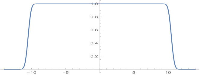
Figure 3: Filter function in $-14<x<14$.

At a leaf node, the integral is computed analytically either using

$$\int_{a}^{b}e^{-x^{2}-2ixt}dx=\frac{1}{2}\sqrt{\pi}\left(\text{Fadd}(ia-t)e^{-a^{2}-2iat}-\text{Fadd}(ib-t)e^{-b^{2}-2ibt}\right)$$

for a boundary node, or

$$\int_{a}^{b}e^{-2ixt}dx=\frac{i}{2t}\left(e^{-2ibt}-e^{-2iat}\right)$$

for an interior node and then evaluated at a set of uniformly distributed $(2M)^{2}$ sample points in $[-14,14]^{2}$ for the two $t$-variables. The function values are then filtered by the pointwise multiplication with the filter function for each variable. The Fourier series of the leaf node function, when needed, can be derived by a $2D$ FFT using the filtered function values. In the formula, we use the Faddeeva function [2, 1, 15, 34] defined as $\text{Fadd}(z)=e^{-z^{2}}\text{erfc}(-iz)$ for a complex number $z$, to avoid the possible overflow/underflow when computing small $e^{-t^{2}}$ times large $\text{erf}(a+it)$ values. An upward pass is then performed to recursively compute the parent’s filtered function $h_{p}$ values at the Fourier interpolation points using its children’s filtered function values at different $t_{l}$, $t_{m}$, and $t_{r}$ interpolation points through 5 steps: (i) multiplying two children’s values at each sample point; (ii) point-wise multiplication with the filter function; (iii) applying the $1D$ fast Fourier transform (FFT) to the $t_{m}$ variable in the region $[-14,14]$ to get the $2M$ Fourier coefficients from the filtered function values at each $t_{l},t_{r}$ interpolation point; (iv) the parent’s $h$-function value at each $t_{l}$ and $t_{r}$ interpolation point is derived by applying the formula

$$\frac{1}{\sqrt{\pi}}\int_{-\infty}^{\infty}e^{-t^{2}}e^{ik\pi t/L}\text{d}t=e^{-\frac{k^{2}\pi^{2}}{4L^{2}}}$$

to integrate the Fourier series expansion of $t_{m}$ variable from (iii) analytically; and (v) the function values will be further filtered. If needed, a $2D$ FFT can be performed to derive the parent’s Fourier series expansion coefficients. Note that the Fourier series in the region $[-14,14]^{2}$ can be extended to the whole space $(-\infty,\infty)^{2}$ as such extension will only introduce an error within machine precision when evaluating the integral in Eq. (7). At the root node, its $h$-function returns the $\phi$ value we are searching for.

The algorithm for efficiently evaluating Eq. (5) can be summarized as the following two passes. In the downward pass, the parent problem is decoupled by applying the Fourier transform to the coupling term, to obtain two child problems. At the finest level, a function with two $t$-variables is created for each leaf node followed by an upward pass to obtains each parent’s function values at the Fourier interpolation points from those of its two children’s functions. At the root level, the constant function (with null $t$-variables) gives the result of the integral in Eq. (5). The recursively implemented Matlab code for the upward pass is presented in Algorithm $1$.

function compute_tri(inode) global NODES %NODES contains the node informations. if NODES(5,inode) == 0, % inode is a leaf node. leafnode(inode); else child1=NODES(5,inode); child2=NODES(6,inode); % find children compute_tri(child1); % find child1’s coefficients. compute_tri(child2); % find child2’s coefficients. % combine children’s coefficients to get parent’s coefficients. if NODES(3,child1)==1 && NODES(3,child2)==2 root(child1,child2); % parent is the root node. elseif NODES(3,child1)==1 && NODES(3,child2)==4 leftbdry(child1,child2); % parent is a left boundary node. elseif NODES(3,child1)==3 && NODES(3,child2)==2 rightbdry(child1,child2); % parent is a right boundary node. else interiornode(child1,child2); % parent is an interior node. end end return end

Table 1: Algorithm 1: Recursive Matlab function for evaluating Eq. (5): upward pass

3.3 Preliminary Numerical Results

We present some preliminary results to demonstrate the accuracy and efficiency of the numerical algorithm for the tridiagonal system in Eq. (5). In the numerical experiments, we set all $a_{i}^{\prime}s$ to $-1$, $b_{1}=0.5$, $b_{2}=2$, and all other $b_{i}^{\prime}s$ to $+1$. We first study the accuracy of the algorithm. For $N=4$, we compute a reference solution using Mathematica with $PrecisionGoal\rightarrow 30$ and $WorkingPrecision\rightarrow 60$, the result is $\phi=2.2893342150887782603$. For $N=8$, Mathematica returns the result $\phi=6.6242487478171897$ with an estimated error $4.25\text{e-}5$, even though $PrecisionGoal\rightarrow 20$ and $WorkingPrecision\rightarrow 40$ are requested. For $N>8$, direct computation using Mathematica simply becomes impossible. In Table 2, we show the Matlab results for different dimensions $N$ and numbers of terms $2M$ in the Fourier series expansion. For all cases, our results converge when $M$ increases. For $N=4$, our result matches Mathematica result to machine precision as soon as enough Fourier terms are used. For $N=8$, our converged results agree with Mathematica result in the first $10$ digits, and we strongly believe our results are more accurate. The numerical tests are performed on a laptop computer with Intel i7-3520M CPU @2.90GHz, with $8.00G$ RAM. For $N=1024$ and $M=512$, approximately $1024\times 1024\times 2047$ function values at the Fourier interpolation points have to be stored in the memory ($\approx 16G$), which exceeds the installed RAM size, hence no result is reported.

$N$	4	8	16
$M$=16	2.326607912389402	6.736597967982384	56.44481808043047
$M$=32	2.289334215119377	6.624246691958165	55.44625398858155
$M$=64	2.289334215088778	6.624246691490006	55.44625397830180
$M$=128	2.289334215088779	6.624246691490009	55.44625397830178
$M$=256	2.289334215088778	6.624246691490005	55.44625397830176
$M$=512	2.289334215088778	6.624246691490003	55.44625397830172
$N$	32	64	1024
$M$=16	3962.697712673563	19531008.87334120	1.182324449792241e+118
$M$=32	3884.575992952042	19067179.07844248	1.019931849681238e+118
$M$=64	3884.575991340509	19067179.06178229	1.019931834748418e+118
$M$=128	3884.575991340506	19067179.06178229	1.019931834748411e+118
$M$=256	3884.575991340500	19067179.06178224	1.019931834748369e+118
$M$=512	3884.575991340498	19067179.06178220	N/A

Table 2: Computed $\phi$ values for different dimensions and number of Fourier terms.

We demonstrate the efficiency of our algorithm by presenting the Matlab simulation time for different dimensions. In the experiment, we present the CPU times for different $M$ and $N$ values, and the unit is in seconds. Clearly, the CPU time grows approximately linearly as the dimension $N$ increases. As a 3-variable {$t_{l}$, $t_{m}$, and $t_{r}$} function has to be processed in the current implementation when finding the parent’s values at the Fourier interpolation points, the CPU time grows approximately by a factor of $8$ as $M$ doubles. For $N=2048$ and $M=256$, approximately $8G$ memory is required, which exceeds the maximum available RAM size, hence no result is reported.

$N$	4	8	16	32	64
$M=32$ CPU time	0.02	0.04	0.15	0.34	0.80
$M=64$ CPU time	0.06	0.27	0.96	2.26	4.60
$M=128$ CPU time	0.12	2.15	6.81	16.5	39.1
$M=256$ CPU time	0.24	12.5	49.1	130	315
$N$	128	256	512	1024	2048
$M=32$ CPU time	1.95	3.75	8.29	16.6	40.1
$M=64$ CPU time	10.2	23.5	49.2	103	214
$M=128$ CPU time	88.5	228	445	970	1942
$M=256$ CPU time	718	1769	3476	8310	N/A

Table 3: CPU time (in seconds) for different $N$ and $M$ values.

4 Case II: Exponential Matrix

In the second case, we consider a matrix $A$ defined by the exponential covariance function

$$A_{i,j}=e^{-|z_{i}-z_{j}|/\beta},\beta>0.$$

To simplify the discussions, we consider a simple 1D setting from spatial or temporal statistics and assume that the rate of decay $\beta=1$ and each random number $X_{j}$ is observed at a location $z_{j}\in[0,b_{z}]$. We assume the $z$-locations $\{z_{j}\in[0,b_{z}]$, $j=1,\ldots,N=2^{P}\}$ are ordered from smallest to largest and the matrix entries are ordered accordingly. We demonstrate how to evaluate the $N$-dimensional integral

(8) $$\phi(\mathbf{a},\mathbf{b};A)=\int_{\mathbf{a}}^{\mathbf{b}}f(\mathbf{x}|A)\text{d}\mathbf{x}=\int_{a_{1}}^{b_{1}}\cdots\int_{a_{N}}^{b_{N}}\exp\left(-\frac{1}{2}\mathbf{x}^{T}A\mathbf{x}\right)\text{d}x_{N}\cdots\text{d}x_{1},$$

for the given constant vectors $\mathbf{a}$ and $\mathbf{b}$ using $O(N)$ operations. Results for different $\beta$ values can be derived by rescaling the $z$-locations and $x$-variables. The presented algorithm can be easily generalized to $\int_{\mathbf{a}}^{\mathbf{b}}H(\mathbf{x})f(\mathbf{x}|A)\text{d}\mathbf{x}$ when $H(\mathbf{x})$ is a low-rank function.

Similar to the tridiagonal matrix case, we generate a binary tree by recursively dividing the parent’s $z$-location set (or equivalently the $x$-variable set) into two child subsets, each containing exactly half of its parent’s points. The hierarchical binary tree is then reflected as a hierarchical matrix as demonstrated in Fig. 1. Unlike the (uniform) binary tree generated for the $z$-location set, the corresponding structure in the matrix sub-division process can be considered as an adaptive quad-tree, where only the diagonal blocks of the matrix are subdivided. Once an off-diagonal block is generated, it becomes a leaf node and no further division is required. Because of the hierarchical structure of the matrix and the low-rank properties of the off-diagonal blocks (which will be discussed next), the exponential matrix is a special $\mathcal{H}$-matrix.

4.1 Divide and Conquer on a Hierarchical Tree

Unlike the tridiagonal system, each off-diagonal matrix in this case is a dense matrix. For this exponential matrix, all the off-diagonal matrices are rank-1 matrices, which can be seen from the separation of variables

$$e^{-|z-y|}=\left\{\begin{array}[]{l}e^{-z}e^{y},\quad z\geq y\\ e^{z}e^{-y},\quad z<y\end{array}\right.$$

In matrix language, the off-diagonal block $A_{1,3}$ can be written as

(9) $$[A_{1,3}(y_{i},z_{j})]=[e^{-y_{N/2+1}},\ldots,e^{-y_{N}}]^{T}[e^{z_{1}},\ldots,e^{z_{N/2}}]$$

for $i=N/2+1,\ldots,N$ and $j=1,\ldots,N/2$. The singular value decomposition of $A_{1,3}$ can be easily derived using Eq. (9) as

$$A_{1,3}=\mathbf{u}\lambda\mathbf{v}^{T}$$

where the left and right singular vectors $\mathbf{u}$ and $\mathbf{v}$ are of size $\frac{N}{2}\times 1$ and respectively the normalized vectors of the discretized functions $e^{-y}$ and $e^{z}$.

When the $x$-variables are divided into $2$ subsets $\mathbf{x}_{1,1}$ and $\mathbf{x}_{1,2}$, the root matrix $A$ can be subdivided accordingly into $4$ blocks

$$A=\begin{bmatrix}A_{1,1}&A_{1,2}=\mathbf{v}\lambda\mathbf{u}^{T}\\ A_{1,3}=\mathbf{u}\lambda\mathbf{v}^{T}&A_{1,4}\end{bmatrix},\mathbf{x}=\begin{bmatrix}\mathbf{x}_{1,1}\\ \mathbf{x}_{1,2}\end{bmatrix},$$

where the first index of $A_{i,j}$ is the current level of the block matrix and the second index is its order in this level. Same indexing rules are used for the $z$-locations and $x$-variables. Completing the square, the quadratic form in the integrand can be reformulated as

$$\begin{array}[]{rcl}\mathbf{x}^{T}A\mathbf{x}&=&\mathbf{x}_{1,1}^{T}A_{1,1}\mathbf{x}_{1,1}+{\color[rgb]{0,0,1}\mathbf{x}_{1,1}^{T}\mathbf{v}\lambda\mathbf{u}^{T}\mathbf{x}_{1,2}+\mathbf{x}_{1,2}^{T}\mathbf{u}\lambda\mathbf{v}^{T}\mathbf{x}_{1,1}}+\mathbf{x}_{1,2}^{T}A_{1,4}\mathbf{x}_{1,2}\\ &=&\mathbf{x}_{1,1}^{T}A_{1,1}\mathbf{x}_{1,1}+\mathbf{x}_{1,2}^{T}A_{1,4}\mathbf{x}_{1,2}+{\color[rgb]{1,0,0}\left((\gamma\mathbf{u}^{T}\mathbf{x}_{1,2}+\frac{1}{\gamma}\mathbf{v}^{T}\mathbf{x}_{1,1})\sqrt{\lambda}\right)^{2}}\\ &&-{\color[rgb]{0,0,1}\mathbf{x}_{1,2}^{T}\gamma^{2}\mathbf{u}\lambda\mathbf{u}^{T}\mathbf{x}_{1,2}}-{\color[rgb]{0,0,1}\mathbf{x}_{1,1}^{T}\frac{1}{\gamma^{2}}\mathbf{v}\lambda\mathbf{v}^{T}\mathbf{x}_{1,1}}\\ &=&{\color[rgb]{0,1,0}\mathbf{x}_{1,1}^{T}(A_{1,1}-\frac{1}{\gamma^{2}}\mathbf{v}\lambda\mathbf{v}^{T})\mathbf{x}_{1,1}}+{\color[rgb]{0,1,0}\mathbf{x}_{1,2}^{T}(A_{1,4}-\gamma^{2}\mathbf{u}\lambda\mathbf{u}^{T})\mathbf{x}_{1,2}}\\ &&+{\color[rgb]{1,0,0}\left((\gamma\mathbf{u}^{T}\mathbf{x}_{1,2}+\frac{1}{\gamma}\mathbf{v}^{T}\mathbf{x}_{1,1})\sqrt{\lambda}\right)^{2}}\\ \end{array}$$

where the first two green terms are the child problems to be processed recursively at finer levels in the divide-and-conquer strategy, $\gamma$ is a constant to be determined, and the last red term shows how the two child problems are coupled. Similar to the tridiagonal case, by introducing a single $t$-variable and applying the Fourier transform formula in Eq. (6) to the coupling term (in red), we get

$$\begin{array}[]{l}\int_{\mathbf{a}}^{\mathbf{b}}e^{-\frac{1}{2}\mathbf{x}^{T}A\mathbf{x}}\text{d}\mathbf{x}=c\int_{-\infty}^{\infty}e^{-t^{2}}h_{1,1}(t)h_{1,2}(t)\text{d}t\end{array}$$

where $h_{1,1}(t)$ and $h_{1,2}(t)$ are the single $t$-variable functions for the two child nodes given by

(10) $$\begin{array}[]{l}h_{1,1}(t)=\int_{a_{1}}^{b_{1}}\cdots\int_{a_{k}}^{b_{k}}e^{-\frac{1}{2}\mathbf{x}_{1,1}^{T}(A_{1,1}-\frac{\lambda}{\gamma^{2}}\mathbf{v}\mathbf{v}^{T})\mathbf{x}_{1,1}+it\frac{\sqrt{2\lambda}}{\gamma}\mathbf{v}^{T}\mathbf{x}_{1,1}}\text{d}\mathbf{x}_{1,1},\\ h_{1,2}(t)=\int_{a_{k+1}}^{b_{k+1}}\cdots\int_{a_{N}}^{b_{N}}e^{-\frac{1}{2}\mathbf{x}_{1,2}^{T}(A_{1,4}-\gamma^{2}\lambda\mathbf{u}\mathbf{u}^{T})\mathbf{x}_{1,2}-it\sqrt{2\lambda}\gamma\mathbf{u}^{T}\mathbf{x}_{1,2}}\text{d}\mathbf{x}_{1,2}.\end{array}$$

Note that the $x$-variables are completely decoupled in the two child problems, and the coupling is now through the $t$-variable.

In order to have a divide-and-conquer algorithm on the hierarchical tree structure, the two child problems should have the following properties:

• By properly choosing the parameter $\gamma$, the new matrices $A_{1,1}-\frac{\lambda}{\gamma^{2}}\mathbf{v}\mathbf{v}^{T}$ and $A_{1,4}-\gamma^{2}\lambda\mathbf{u}\mathbf{u}^{T}$ should be symmetric positive definite; and

• The off-diagonal blocks of these new matrices should be low-rank.

We found that the choice of $\gamma$ is not unique, and there exist a range of $\gamma$ values for the child problems to have these properties. The choice of $\gamma$ is addressed next.

4.2 Potential Theory based Analysis

In this section, we apply the potential theory from the analysis of ordinary and partial differential equations and show how the divide-and-conquer strategy can be successfully performed on the hierarchical tree structure. Purely numerical linear algebra based approaches for more general cases will be briefly addressed later.

4.2.1 Green’s Functions

We present the results for $b_{z}=1$ to simplify the notations and assume $z_{j}\in[0,1]$. We start from the observation that

$$G(z,y)=\frac{1}{2}e^{-|z-y|}=\left\{\begin{array}[]{l}coef\cdot g_{r}(z)\cdot g_{l}(y),\quad z\geq y,\\ coef\cdot g_{r}(y)\cdot g_{l}(z),\quad z<y\end{array}\right.$$

is the domain Green’s function of the ordinary differential equation (ODE) two-point boundary value problem

(11) $$\left\{\begin{array}[]{l}u(z)-u^{\prime\prime}(z)=f(z),\quad z\in[0,1],\\ u(0)=u^{\prime}(0),\quad u(1)=-u^{\prime}(1),\end{array}\right.$$

where $coef=\frac{1}{2}$, $g_{l}(z)=e^{z-1}$ and $g_{r}(z)=e^{1-z}$. The proof is simply a straightforward validation that $u(z)=\int_{0}^{1}G(z,y)f(y)dy$ satisfies both the ODE and boundary conditions.

In the following discussions, we consider the continuous version of the original matrix problem, where the matrix $A$ is the discretized Green’s function $G(z,y)$, the two off-diagonal submatrices $A_{1,2}$ and $A_{1,3}$ are the discretized $g_{r}(z)\cdot g_{l}(y)$ and $g_{r}(y)\cdot g_{l}(z)$, respectively. Some simple algebra manipulations show that the submatrices $A_{1,1}-\frac{\lambda}{\gamma^{2}}\mathbf{v}\mathbf{v}^{T}$ and $A_{1,4}-\gamma^{2}\lambda\mathbf{u}\mathbf{u}^{T}$ can be considered as the discretized $G(z,y)-\tilde{\gamma}^{2}\cdot g_{l}(z)\cdot g_{l}(y)$ and $G(z,y)-\frac{1}{\tilde{\gamma}^{2}}\cdot g_{r}(z)\cdot g_{r}(y)$, and the coefficients $it\frac{\sqrt{2\lambda}}{\gamma}\mathbf{v}^{T}$ and $it\sqrt{2\lambda}\gamma\mathbf{u}^{T}$ for the linear terms of the $x$-variables $\mathbf{x}_{1,1}$ and $\mathbf{x}_{1,2}$ in Eq. (10) are the discretized $it\tilde{\gamma}g_{l}(z)$ and $it\frac{1}{\tilde{\gamma}}g_{r}(z)$, respectively.

Remark: The observation also allows easy proof of the positive definiteness of the matrix $A$, which is the discretized Green’s function $G(z,y)$. In order to show that for any vector $\mathbf{f}\neq\bf{0}$, the quadratic form satisfies $\frac{1}{2}\mathbf{f}^{T}A\mathbf{f}>0$, we consider its continuous version defined as

$$\int_{0}^{1}f(z)\left(\int_{0}^{1}G(z,y)f(y)dy\right)dz=\int_{0}^{1}f(z)u(z)dz$$

where $u(z)=\int_{0}^{1}G(z,y)f(y)dy$ and $f(y)$ is the continuous version of the (discretized) vector $\mathbf{f}$. As $f(z)=u(z)-u^{\prime\prime}(z)$, applying the integration by parts, we have

$$\int_{0}^{1}f(z)u(z)dz=\int_{0}^{1}\left(u^{2}(z)+(u^{\prime}(z))^{2}\right)dz-u^{\prime}(1)\cdot u(1)+u^{\prime}(0)\cdot u(0).$$

As $f(z)\neq 0$, therefore $u(z)\neq 0$, and applying the boundary conditions of the ODE, we have $\int_{0}^{1}f(z)u(z)dz>0$. We refer to the two-variable function $G(z,y)$ as a positive definite function. The positive definiteness of the matrix $A$ can be proved in a similar way using the discretized integration by parts.

A particular choice of $\gamma$ can be determined by considering the corresponding child ODE problems as follows. We first study the root problem and define its two children as the left child and right child, and the locations $z_{i}$ of the left child and $z_{j}$ of the right child satisfy the condition $z_{i}<z_{j}$ as the $z$-locations of the $x$-variables in the two child problems are separated and ordered. We pick a location $\zeta$ between the two clusters of $z$-locations. Note that the choice of $\zeta$ is not unique. We have the following results for the root node.

Theorem 4.1.

If we choose $\tilde{\gamma}=\frac{e^{-\zeta}}{\sqrt{2}}$, then

• for the left child, the new function $G_{l}(z,y)=G(z,y)-\tilde{\gamma}^{2}\cdot g_{l}(z)\cdot g_{l}(y)$ is the Green’s function of the ODE problem

  $$\left\{\begin{array}[]{l}\mathbf{u}_{1}(z)-\mathbf{u}_{1}^{\prime\prime}(z)=f(z),\quad z\in[0,\zeta],\\ \mathbf{u}_{1}(0)=\mathbf{u}_{1}^{\prime}(0),\quad\mathbf{u}_{1}(\zeta)=0.\end{array}\right.$$

  The function $G_{l}(z,y)$ is positive definite.

• For the right child, the new function $G_{r}(z,y)=G(z,y)-\frac{1}{\tilde{\gamma}^{2}}\cdot g_{r}(z)\cdot g_{r}(y)$ is the Green’s function of the ODE problem

  $$\left\{\begin{array}[]{l}\mathbf{u}_{2}(z)-\mathbf{u}_{2}^{\prime\prime}(z)=f(z),\quad z\in[\zeta,1],\\ \mathbf{u}_{2}(\zeta)=0,\quad\mathbf{u}_{2}(1)=-\mathbf{u}_{2}^{\prime}(1).\end{array}\right.$$

  The function $G_{r}(z,y)$ is positive definite.

• The two child ODE problem solutions $\mathbf{u}_{1}(z)$ and $\mathbf{u}_{2}(z)$ can be derived by subtracting a single layer potential defined at $z=\zeta$ from the parent’s solution $u(z)$ of Eq. (11), so that solutions $\mathbf{u}_{1}(z)$ and $\mathbf{u}_{2}(z)$ satisfy the zero interface condition at $z=\zeta$. The other boundary condition for each child ODE problem is the same as its parent’s boundary condition.

These results can be easily validated by plugging in the functions to the ODE problems. The positive definiteness of the child Green’s function can be proved using the same integration by part technique as we did for the parent’s Green’s function.

For a general parent node on the tree structure, we have the following generalized results.

Theorem 4.2.

Consider a parent node with the corresponding function $G_{p}(z,y)$ defined on the interval $[a,b]$, and $\zeta$ is a point separating the two children’s $z$-locations. Then there exists a number $\tilde{\gamma}$ which depends on $\zeta$, such that

• for the left child, the new function $G_{l}(z,y)=G(z,y)-\tilde{\gamma}^{2}\cdot g_{l}(z)\cdot g_{l}(y)$ is the Green’s function of the ODE problem

  $$\left\{\begin{array}[]{l}\mathbf{u}_{1}(z)-\mathbf{u}_{1}^{\prime\prime}(z)=f(z),\quad z\in[a,\zeta],\\ \mbox{same boundary condition as parent at $x=a$, and }\mathbf{u}_{1}(\zeta)=0.\end{array}\right.$$

  The function $G_{l}(z,y)$ is positive definite.

• For the right child, the new function $G_{r}(z,y)=G(z,y)-\frac{1}{\tilde{\gamma}^{2}}\cdot g_{r}(z)\cdot g_{r}(y)$ is the Green’s function of the ODE problem

  $$\left\{\begin{array}[]{l}\mathbf{u}_{2}(z)-\mathbf{u}_{2}^{\prime\prime}(z)=f(z),\quad z\in[\zeta,b],\\ \mathbf{u}_{2}(\zeta)=0,\mbox{ and same boundary condition as parent at $x=b$}.\end{array}\right.$$

  The function $G_{r}(z,y)$ is positive definite.

• The two child ODE problem solutions $\mathbf{u}_{1}(z)$ and $\mathbf{u}_{2}(z)$ can be derived by subtracting a single layer potential defined at $z=\zeta$ from the parent’s solution $u(z)$ of Eq. (11), so that solutions $\mathbf{u}_{1}(z)$ and $\mathbf{u}_{2}(z)$ satisfy the zero interface condition at $z=\zeta$. The other boundary condition for each child ODE problem is the same as its parent’s boundary condition.

The detailed formulas for the number $\tilde{\gamma}$ and Green’s functions are presented in the Appendix. The proof of the theorem is simply validations of the formulas.

4.2.2 Parent-children Relations

In the matrix form, for a general parent node at level $l$ in the hierarchical tree structure with left child $1$ and right child $2$, its $h$-function

(12) $$h_{p}(\mathbf{t}_{p})=\int_{\mathbf{a}_{p}}^{\mathbf{b}_{p}}e^{-\frac{1}{2}\mathbf{x}_{p}^{T}A_{p}\mathbf{x}_{p}}e^{i\mathbf{t}_{p}^{T}D_{p}\mathbf{x}_{p}}\text{d}\mathbf{x}_{p}$$

can be decomposed into two child problems as

$$h_{p}(\mathbf{t}_{p})=\frac{1}{\sqrt{\pi}}\int_{-\infty}^{\infty}e^{-t_{new}^{2}}h_{1}(\mathbf{t}_{1})h_{2}(\mathbf{t}_{2})\text{d}t_{new},$$

where

(13) $$\begin{array}[]{l}h_{1}(\mathbf{t}_{1})=\int_{\mathbf{a}_{1}}^{\mathbf{b}_{1}}e^{-\frac{1}{2}\mathbf{x}_{1}^{T}A_{1}\mathbf{x}_{1}}e^{it_{new}\tilde{\gamma}\mathbf{g}_{l}^{T}(\mathbf{z}_{1})\cdot\mathbf{x}_{1}}e^{i\mathbf{t}_{p}^{T}D_{p,1}\mathbf{x}_{1}}\text{d}\mathbf{x}_{1}=\int_{\mathbf{a}_{1}}^{\mathbf{b}_{1}}e^{-\frac{1}{2}\mathbf{x}_{1}^{T}A_{1}\mathbf{x}_{1}}e^{i\mathbf{t}_{1}^{T}D_{1}\mathbf{x}_{1}}\text{d}\mathbf{x}_{1},\\ h_{2}(\mathbf{t}_{2})=\int_{\mathbf{a}_{2}}^{\mathbf{b}_{2}}e^{-\frac{1}{2}\mathbf{x}_{1}^{T}A_{2}\mathbf{x}_{1}}e^{it_{new}\frac{1}{\tilde{\gamma}}\mathbf{g}_{r}^{T}(\mathbf{z}_{2})\cdot\mathbf{x}_{2}}e^{i\mathbf{t}_{p}^{T}D_{p,2}\mathbf{x}_{2}}\text{d}\mathbf{x}_{2}=\int_{\mathbf{a}_{2}}^{\mathbf{b}_{2}}e^{-\frac{1}{2}\mathbf{x}_{2}^{T}A_{2}\mathbf{x}_{2}}e^{i\mathbf{t}_{2}^{T}D_{2}\mathbf{x}_{2}}\text{d}\mathbf{x}_{2}.\end{array}$$

In the formulas, $\mathbf{t}_{p}$ is the vector containing all the $t$-variables introduced at coarser levels to subdivide $p$’s parents’ $h$-functions. $\mathbf{x}_{p}=[\mathbf{x}_{1};\mathbf{x}_{2}]$, $\mathbf{x}_{1}$, and $\mathbf{x}_{2}$ are respectively the vectors containing the $x$-variables of the parent $p$, child $1$, and child $2$. {$\mathbf{a}_{p}$,$\mathbf{b}_{p}$}, {$\mathbf{a}_{1}$,$\mathbf{b}_{1}$}, and {$\mathbf{a}_{2}$,$\mathbf{b}_{2}$} are respectively the lower and upper integration bounds of $\mathbf{x}_{p}$, $\mathbf{x}_{1}$, and $\mathbf{x}_{2}$. $A_{p}=\left[\begin{array}[]{cc}A_{l,1}&A_{l,2}\\ A_{l,3}&A_{l,4}\end{array}\right]$, $A_{1}$, and $A_{2}$ are respectively the discretized Green’s functions of the parent $p$, child $1$, and child $2$, which satisfy

$$A_{1}=A_{l,1}-\tilde{\gamma}^{2}\cdot\mathbf{g}_{l}(\mathbf{z}_{1})\cdot\mathbf{g}_{l}^{T}(\mathbf{z}_{1}),\quad A_{2}=A_{l,4}-\frac{1}{\tilde{\gamma}^{2}}\cdot\mathbf{g}_{r}(\mathbf{z}_{2})\cdot\mathbf{g}_{r}^{T}(\mathbf{z}_{2}),$$

$\mathbf{z}_{p}=[\mathbf{z}_{1};\mathbf{z}_{2}]$, $\mathbf{z}_{1}$, and $\mathbf{z}_{2}$ are respectively the $z$-location vectors of the parent $p$ and child $1$ and $2$, and $\mathbf{g}_{l}(\mathbf{z}_{1})$ and $\mathbf{g}_{r}(\mathbf{z}_{2})$ are the discrete function values of $g_{l}(z)$ and $g_{r}(z)$ in the Green’s functions evaluated at different $z$-locations. $\mathbf{t}_{p}^{T}D_{p}\mathbf{x}_{p}$ is a scalar term representing the linear combinations of the $t_{k}\cdot x_{j}$ terms, and by separating the $x$-variables, it can be written as

$$\mathbf{t}_{p}^{T}D_{p}\mathbf{x}_{p}=\mathbf{t}_{p}^{T}D_{p,1}\mathbf{x}_{1}+\mathbf{t}_{p}^{T}D_{p,2}\mathbf{x}_{2}.$$

After introducing the new $t$-variable $t_{new}$ to divide the parent’s problem to two subproblems of child $1$ and child $2$, each with half of the parent $p$’s $x$-variables, we have $\mathbf{t}_{1}=[\mathbf{t}_{p};t_{new}]$, $\mathbf{t}_{2}=[\mathbf{t}_{p};t_{new}]$, and

(14) $$\left\{\begin{array}[]{l}\mathbf{t}_{1}^{T}D_{1}\mathbf{x}_{1}=\mathbf{t}_{p}^{T}D_{p,1}\mathbf{x}_{1}+t_{new}\tilde{\gamma}\mathbf{g}_{l}^{T}(\mathbf{z}_{1})\cdot\mathbf{x}_{1},\\ \mathbf{t}_{2}^{T}D_{2}\mathbf{x}_{2}=\mathbf{t}_{p}^{T}D_{p,2}\mathbf{x}_{2}+t_{new}\frac{1}{\tilde{\gamma}}\mathbf{g}_{r}^{T}(\mathbf{z}_{2})\cdot\mathbf{x}_{2}.\end{array}\right.$$

For the root node, $A_{p}$ is the given matrix $A$ and $\mathbf{t}_{p}$ is an empty set. At a leaf node, we have

$$h_{leaf}(\mathbf{t}_{leaf})=\int_{a_{k}}^{b_{k}}e^{-\frac{1}{2}\alpha_{k}x_{k}^{2}}e^{i(\mathbf{t}_{leaf}^{T}D_{leaf})x_{k}}\text{d}x_{k}$$

where $D_{leaf}$ is a column vector of the same size as $\mathbf{t}_{leaf}$ (the size equals to the number of levels in the hierarchical tree structure). Analytical formula is available for $h_{leaf}(\mathbf{t}_{leaf})$ using

(15) $$\int_{a}^{b}e^{-x^{2}}e^{-2itx}\,\text{d}x=\frac{1}{2}\sqrt{\pi}e^{-t^{2}}(\text{erf}(b+it)-\text{erf}(a+it)).$$

4.2.3 Dimension Reduction and Effective Variables

Note that for a node at level $l$, its $h$-function $h(\mathbf{t})$ will contain as many as $l$ $t$-variables introduced at parent levels. Therefore for a $N$-dimensional problem, the number of $t$-variables for a leaf node can be as many as $\log(N)$. However, inspecting the term $(\mathbf{t}_{leaf}^{T}D_{leaf})x_{k}$ for the function $h_{leaf}(\mathbf{t}_{leaf})$, if one introduces a new single variable $w=\mathbf{t}_{leaf}^{T}D_{leaf}$, then $h_{leaf}$ is effectively a single variable function of $w$. We therefore study the effective variables and their properties in this section.

From Eq. (14), we see that when a new $t$-variable $t_{new}$ is introduced to divide the parent problem into two child problems, the additional terms added to the linear terms of the $x$-variables in the exponent are $t_{new}\tilde{\gamma}\mathbf{g}_{l}^{T}(\mathbf{z}_{1})\cdot\mathbf{x}_{1}$ for child $1$ and $t_{new}\frac{1}{\tilde{\gamma}}\mathbf{g}_{r}^{T}(\mathbf{z}_{2})\cdot\mathbf{x}_{2}$ for child $2$, where $\mathbf{g}_{l}(\mathbf{z}_{1})$ and $\mathbf{g}_{r}(\mathbf{z}_{2})$ are the discrete function values of $g_{l}(z)$ and $g_{r}(z)$ in the Green’s functions evaluated at different $z$-locations. For all the Green’s functions, $g_{l}(z)$ and $g_{r}(z)$ are always a combination of the basis functions $e^{z}$ and $e^{-z}$. This can be seen either from the ODE problems or from the Green’s functions in the Appendix. Therefore, switching the basis to $e^{z}$ and $e^{-z}$, the term $\mathbf{t}^{T}D\mathbf{x}$ can always be written as

(16) $$\mathbf{t}^{T}D\mathbf{x}=(w_{1}e^{\mathbf{z}}+w_{2}e^{-\mathbf{z}})^{T}\cdot\mathbf{x},$$

where $e^{\mathbf{z}}$ and $e^{-\mathbf{z}}$ are the vectors derived by evaluating the functions $e^{z}$ and $e^{-z}$ at the $z$-locations. Clearly, after this change of variables from $t$-variables to {$w_{1}$, $w_{2}$}, each $h$-function is effectively a function with no more than $2$ variables. We define $w_{1}$ and $w_{2}$ as the effective $w$-variables.

Our numerical experiments show that at finer levels of the hierarchical tree structure when the interval size of the tree node becomes smaller, the two basis functions $e^{z}$ and $e^{-z}$ are closer to linear dependent which will cause numerical stability issues. For better stability properties, orthogonal or near orthogonal basis functions are used. A sample basis is $\{\Phi_{1}(z)=\cosh(z-c),\Phi_{2}(z)=\frac{\sinh(z-c)}{b-a}\}$ when the $z$-locations of the $x$-variables are in the interval $[a,b]$. When $c$ is the center of the interval, the two functions are orthogonal to each other when measured using the standard $L_{2}$ norm with a constant weight function. For a parent node with effective $w$-variables $\{w_{1}^{p},w_{2}^{p}\}$ and basis functions $\{\mathbf{\Phi}_{1}^{p},\mathbf{\Phi}_{2}^{p}\}$, where the vector $\mathbf{\Phi}$ represents the discretized $\Phi(z)$ at the $z$-locations, in the divide-and-conquer strategy, the effective $w$-variables should satisfy the relations

(17) $$\left\{\begin{array}[]{l}w_{1}^{p}\Phi_{1}^{p}+w_{2}^{p}\Phi_{2}^{p}+t_{new}\tilde{\gamma}g_{l}(z)=w_{1}^{1}\Phi_{1}^{1}+w_{2}^{1}\Phi_{2}^{1},\\ w_{1}^{p}\Phi_{1}^{p}+w_{2}^{p}\Phi_{2}^{p}+t_{new}\frac{1}{\tilde{\gamma}}g_{r}(z)=w_{1}^{2}\Phi_{1}^{2}+w_{2}^{2}\Phi_{2}^{2},\end{array}\right.$$

where $\{\Phi_{1}^{p},\Phi_{2}^{p}\}$, $\{\Phi_{1}^{1},\Phi_{2}^{1}\}$, $\{\Phi_{1}^{2},\Phi_{2}^{2}\}$ are respectively the continuous basis for the parent, child 1, and child 2, $\{w_{1}^{1},w_{2}^{1}\}$ and $\{w_{1}^{2},w_{2}^{2}\}$ are the effective $w$-variables of child $1$ and child $2$ for the discrete basis vectors $\{\mathbf{\Phi}_{1}^{1},\mathbf{\Phi}_{2}^{1}\}$ and $\{\mathbf{\Phi}_{1}^{2},\mathbf{\Phi}_{2}^{2}\}$, respectively. In the Appendix, we present the detailed formulas demonstrating the relations between parent $p$’s and children’s effective $w$-variables for the basis choice {$\cosh(z-c)$, $\frac{\sinh(z-c)}{b-a}$}.

In the tridiagonal case discussed in Section 3, we only need to study the $h$-functions when their $t$-variables satisfy $|t_{j}|<7$, as outside the interval the integrand value is controlled by the factor $e^{-t_{j}^{2}}$ and hence can be neglected. Similar results can be obtained for the exponential case, when a proper set of basis is chosen. Assuming all the $z$-locations are approximately uniformly distributed in the interval $[0,1]$, we have the following theorem for the effective $w$-variables $w_{1}$ and $w_{2}$.

Theorem 4.3.

Assume the $N\times N$ matrix $A$ is defined by the exponential covariance function, the $z$-locations are uniformly distributed in the interval $[0,1]$, and all the $t$-variables satisfy $|t_{j}|<7$. When the basis functions are chosen as $\{\Phi_{1}(z)=\cosh(z-c),\Phi_{2}(z)=\frac{\sinh(z-c)}{b-a}\}$ for each tree node, then there exists a constant $C$ independent of $N$, such that the corresponding effective $w$-variables $w_{1}$ and $w_{2}$ (combinations of the $t$-variables) satisfy the conditions $|w_{1}|\leq C$ and $|w_{2}|\leq C$.

The proof of this theorem is simply the leading order analysis of the parent-children effective $w$-variable relations, and the fact that $\cos(h)=1+\frac{h^{2}}{2}+O\left(h^{4}\right)$, $\frac{\sinh(h)}{2h}=\frac{1}{2}+\frac{h^{2}}{12}+O\left(h^{4}\right)$, $\sinh\left(\frac{h}{2}\right)\sqrt{\sinh(h)\text{csch}(2h)\text{csch}(h)}=\frac{\sqrt{h}}{2\sqrt{2}}-\frac{7h^{5/2}}{48\sqrt{2}}+O\left(h^{9/2}\right)$, and $\sum_{k=0}^{L}\sqrt{\frac{1}{2^{k}}}<\sqrt{2}+2$, where $L$ is the number of levels in the tree structure. We skip the proof details. Interested readers can request a copy of our Mathematica file for further details. We point out that when the basis functions are chosen as $\{e^{z},e^{-z}\}$, the effective $w$-variables become unbounded.

Remark: In the numerical implementation, instead of using the upper bound $C$ for a tree node $j$, the ranges $C_{1}^{j}$ and $C_{2}^{j}$ of the effective $w$-variables $w_{1}$ and $w_{2}$ are computed using the parent-children effective $w$-variable relations in Eq. (17) and stored in the memory. Similar to the tridiagonal case, a filter function is applied to the $h$-functions so that the filtered function smoothly decays to zero in the region $|w_{1}|\in[C_{1},2C_{1}]$ or $|w_{2}|\in[C_{2},2C_{2}]$, see Fig. 3. Then the Fourier series of the filtered $h$-function is constructed in the region $[-2C_{1},2C_{1}]\times[-2C_{2},2C_{2}]$, and finally the constructed Fourier series is expanded to the whole space when deriving parent’s $h$-function values. In the algorithm implementation, when the uniform FFT [14] can no longer be applied, we use the open source NUFFT package developed in [24, 36] to accelerate the computation of the Fourier series.

4.3 Pseudo-algorithm

Similar to the tridiagonal case, the algorithm can be summarized as the following two passes: In the downward pass, the parent problem is decoupled by applying the Fourier transform to the coupling term, to obtain two child problems. Six coefficients $\{c_{1},c_{2},c_{3},c_{4},c_{5},c_{6}\}$ are derived so that the effective $w$-variables of the current node satisfy

(18) $$w_{1}=c_{1}w_{1}^{p}+c_{2}w_{2}^{p}+c_{3}t_{new},\quad w_{2}=c_{4}w_{1}^{p}+c_{5}w_{2}^{p}+c_{6}t_{new},$$

where $w_{1}^{p}$ and $w_{2}^{p}$ are the parent’s effective $w$-variables. Also, the ranges $C_{1}$ and $C_{2}$ of the effective $w$-variables $w_{1}$ and $w_{2}$ are computed. A total of $8$ numbers are stored for each node. Note that both the storage and number of operations are constant for each tree node. The pseudo-algorithm is presented in Algorithm $2$, where the details of computing the $8$ numbers for each node is presented in the Appendix.

function compexp_downward(inode) global NODES %NODES contains the node informations. global TRANSCoef %TRANSCoef contains the $8$ numbers. if NODES(5,inode) == 0, % inode is a leaf node. return; else child1=NODES(5,inode); child2=NODES(6,inode); % find children compute the $8$ numbers using the formulas in Appendix for inode is a root, left boundary, right boundary, or interior node. compexp_downward(child1); % find child 1’s $8$ numbers. compexp_downward(child2); % find child 2’s $8$ numbers. end return end

Table 4: Algorithm 2: Recursive Matlab function for exponential case: downward pass

At the finest level, a function with one effective variable is constructed analytically using Eq. (15). A numerically equivalent two-variable $\{w_{1}^{leaf},w_{2}^{leaf}\}$ Fourier series expansion is then constructed by evaluating the analytical solution at the interpolation points, applying the filter function, and then applying FFT to derive the $2D$ Fourier series expansion which is considered valid in the whole space. An upward pass is then performed, to obtains each parent’s Fourier coefficients from those of its two children’s functions. For each parent node, we first replace the child’s effective $w$-variables with $w_{1}^{p}$, $w_{2}^{p}$ and $t_{new}$ using Eq. (18) and the $6$ numbers from the downward pass, then evaluate each child’s global Fourier series at the uniform interpolation points of $w_{1}^{p}$, $w_{2}^{p}$ and $t_{new}$ (determined by the ranges $C_{1}$ and $C_{2}$ from the downward pass, we set the range of $t_{new}$ to $7$). In this step, we have to use the NUFFT as the $8$ numbers for different tree nodes are different so the uniform FFT is not applicable. Multiplying the two children’s function values and the filter function values at each interpolation point, we then apply the FFT to the $t_{new}$ variable and derive the Fourier series of $t_{new}$ at each $w_{1}^{p}$ and $w_{2}^{p}$ interpolation point. The integral

$$h_{p}(w_{1}^{p},w_{2}^{p})=\frac{1}{\sqrt{\pi}}\int_{-\infty}^{\infty}e^{-t_{new}^{2}}h_{1}h_{2}\text{d}t_{new}$$

is then evaluated analytically at each $w_{1}^{p}$ and $w_{2}^{p}$ interpolation point. Finally, another 2D FFT is performed to derive the coefficients of $h_{p}$. At the root level, the constant function (with no $t$-variables) gives the result of the integral. In the implementation, as we use unified formulas for both the boundary nodes and interior nodes, the two functions $leftbdry$ and $rightbdry$ become unnecessary, see Appendix for details. Except for the detailed implementations in the functions $leafnode$, $root$, and $interiornode$, the recursively implemented Matlab algorithm for the upward pass is identical in structure as the presented Algorithm $1$ for the tri-diagonal case, we therefore skip the pseudo-code.

The algorithm complexity can be computed as follows. In both the upward pass and downward pass, constant numbers of operations and storage are required for each tree node, the overall algorithm complexity and memory requirement are therefore both asymptotically optimal $O(N)$ for the $N$-dimensional integration problem.

4.4 Preliminary Numerical Results

We present some preliminary results to demonstrate the accuracy and efficiency of the numerical algorithm for the exponential case. The $N$ $z$-location points are randomly chosen in $[0,1]$ and sorted. A uniform tree is then generated by recursively subdividing the $z$-locations and corresponding $x$-variables, and the same settings of $\mathbf{a}$ and $\mathbf{b}$ are used as in the tridiagonal case. We first study the accuracy of the algorithm. For $N=4$, we compute a reference solution $\phi=9.63128791560604001$ using Mathematica, with an estimated error $5.99\text{e-}8$. For $N=8$, Mathematica returns the result $\phi=1.16750673314578e+02$ with an estimated error $0.064$. For $N>8$, direct computation using Mathematica becomes impossible. In Table 5, we show the Matlab results for different dimensions $N$ when $2M$ Fourier series terms are used in the approximation. The error tolerance for the NUFFT solver is set to $1\text{e-}12$. For all cases, our results converge when $M$ increases. For both $N=4$ and $N=8$, our converged results match those from Mathematica within the estimated error from Mathematica.

In the current implementation, as the exponential case involves operations on a 3-variables function $h(w_{1}^{p},w_{2}^{p},t_{new})$ for each child when forming the parent’s Fourier series expansion, while both the storage and operations for the tridiagonal case can be compressed so one only works on 2-variable functions (variables $\{t_{l},t_{m}\}$ for child $1$ and $\{t_{m},t_{r}\}$ for child $2$), the exponential solver therefore requires more operations and memory than the tridiagonal case. We tested our code on a desktop with 16GB memory and Intel Xeon CPU E3-1225 v6 @3.30GHz. For $N=4$ and $M=512$, More than $8G$ memory is already required, hence no result for $M=512$ is reported.

$N$	4	8	16
$M$=16	9.646301617204299	118.8260790816760	21594.43676761628
$M$=32	9.631244805483258	116.7475848966488	17592.18271523017
$M$=64	9.631287915305332	116.7505122381643	17591.75082916860
$M$=128	9.631287915311097	116.7505122544810	17591.75095515863
$M$=256	9.631287915311061	116.7505122544801	17591.75095515877
$N$	32	64	128
$M$=16	1131582930.741270	4.332761307147880e+18	7.074841023044070e+37
$M$=32	550963842.9679267	1.046292247268069e+18	9.380354831605098e+36
$M$=64	540456718.9698794	8.163524406713720e+17	3.432262767034514e+36
$M$=128	540456737.4129881	8.163182314210313e+17	3.394537652388589e+36
$M$=256	540456737.4129064	8.163182314206217e+17	3.394537652164628e+36

Table 5: Computed $\phi$ values for different dimensions and numbers of Fourier terms, exponential case.

Remark: We explain the large errors when $M=16$ (and $M=32$) for large $N$ values. When the dimension of the problem increases, its condition number also increases exponentially. For each leaf node, if we assume the numerical solution has a relative error $\epsilon$ in each leaf node function $h_{leaf}$, in the worst case, the relative error for the $N$ dimensional integral can be approximated by $(1+\epsilon)^{N}-1$ as the $N$ leaf node functions will be “multiplied” together in the upward pass to get the final integral value. Clearly, the condition number of the analytical problem grows exponentially as $N$ increases. In our current implementation, we set the error tolerance of the NUFFT solver to $10^{-12}$ relative error. Therefore, a very rough estimate for the error when $N=128$, assuming $M$ is large enough so the leaf node function $h_{leaf}$ is resolved to machine precision, is given by $(1+10^{-12})^{128}\approx 1+10^{-10}$, i.e., at most $10$ digits are correct if the worst case happens. Our numerical results show that for the same $N$ value, all the converged results match at least in the first $10$ significant digits in Table 5.

We demonstrate the efficiency of our algorithm by presenting the Matlab simulation time for different $M$ and $N$ values, and the unit for the CPU time is in seconds. The current Matlab code has not been fully vectorized or parallelized, and significant performance improvement in the prefactor of the $O(N)$ algorithm is expected from a future optimized code. However, the numerical results in Table 6 using our existing code sufficiently and clearly show the asymptotic algorithm complexity: the CPU time grows approximately linearly as the dimension $N$ increases, and it increases by a factor of approximately $8$ as $M$ doubles.

$N$	4	8	16	32	64
$M=32$ CPU time	1.03	2.96	6.67	14.1	29.2
$M=64$ CPU time	8.06	23.4	53.8	115	238
$M=128$ CPU time	65.2	191	445	949	1965
$N$	128	256	512	1024	2048
$M=32$ CPU time	59.4	119	244	471	951
$M=64$ CPU time	491	988	1924	3889	7766
$M=128$ CPU time	4049	8029	16068	32465	65073

Table 6: CPU time (in seconds) for different $M$ and $N$ values, exponential case.

5 Generalizations and Limitations

In both the tridiagonal and exponential cases, we present the algorithms for the case $H(\mathbf{x})=constant$. For a general $H$ with low-rank properties, i.e.,

$$H(\mathbf{x})=\sum_{p=1}^{P}\prod_{k=1}^{N}u_{p,k}(x_{k}),$$

as $P$ is a small number, we can evaluate the expectation of each $p$ term $\prod_{k=1}^{N}u_{p,k}(x_{k})$ and then add up the results. As the $x$-variables are already separated in the representation, the downward decoupling process can be performed the same as that in the tridiagonal or exponential case. At the finest level, the leaf node’s function $h_{leaf}$ becomes

$$h_{leaf}(\mathbf{t}_{leaf})=\int_{a_{k}}^{b_{k}}u_{p,k}(x_{k})e^{-\frac{1}{2}\alpha_{k}x_{k}^{2}}e^{i(\mathbf{t}_{leaf}^{T}D_{leaf})x_{k}}\text{d}x_{k}.$$

Note that analytical formula is in general not available for $h_{leaf}$, a numerical scheme has to be developed to compute the Fourier coefficients of $h_{leaf}$. This is clearly numerically feasible as the integral is one-dimensional and $h_{leaf}$ is effectively a single variable function.

Next we consider more general $A$ matrices. We restrict our attention to the symmetric positive definite $\mathcal{H}$-matrices, and discuss the required low-rank and low dimensional properties in order for our method to become asymptotically optimal $O(N)$. A minimal requirement from the algorithm is that the off-diagonal matrices should be low rank. Consider a parent’s matrix $A$ with such low rank off-diagonals and the corresponding $x$-variables,

$$A=\begin{bmatrix}A_{l,1}&A_{l,2}=\mathbf{V}\Lambda\mathbf{U}^{T}\\ A_{l,3}=\mathbf{U}\Lambda\mathbf{V}^{T}&A_{l,4}\end{bmatrix},\mathbf{x}=\begin{bmatrix}\mathbf{x}_{l,1}\\ \mathbf{x}_{l,2}\end{bmatrix},$$

where the first index $l$ is the current level of the block matrices and point sets, and we assume $\Lambda$ is low rank, $rank(\Lambda)=P$. Then we can rewrite the quadratic term in the exponent of the integrand as

$$\begin{array}[]{rcl}\mathbf{x}^{T}A\mathbf{x}&=&\mathbf{x}_{l,1}^{T}A_{l,1}\mathbf{x}_{l,1}+{\color[rgb]{0,0,1}\mathbf{x}_{l,1}^{T}\mathbf{V}\Lambda\mathbf{U}^{T}\mathbf{x}_{l,2}+\mathbf{x}_{l,2}^{T}\mathbf{U}\Lambda\mathbf{V}^{T}\mathbf{x}_{l,1}}+\mathbf{x}_{l,2}^{T}A_{l,4}\mathbf{x}_{l,2}\\ &=&{\color[rgb]{1,0,0}(B\mathbf{U}^{T}\mathbf{x}_{l,2}+B^{-T}\mathbf{V}^{T}\mathbf{x}_{l,1})^{T}\Lambda(B\mathbf{U}^{T}\mathbf{x}_{l,2}+B^{-T}\mathbf{V}^{T}\mathbf{x}_{l,1})}+\\ &&\mathbf{x}_{l,1}^{T}A_{l,1}\mathbf{x}_{l,1}-{\color[rgb]{0,0,1}\mathbf{x}_{l,2}^{T}\mathbf{U}B^{T}\Lambda B\mathbf{U}^{T}\mathbf{x}_{l,2}}+\\ &&\mathbf{x}_{l,2}^{T}A_{l,4}\mathbf{x}_{l,2}-{\color[rgb]{0,0,1}\mathbf{x}_{l,1}^{T}\mathbf{V}B^{-1}\Lambda B^{-T}\mathbf{V}^{T}\mathbf{x}_{l,1}}\\ &=&{\color[rgb]{0,1,0}\mathbf{x}_{l,1}^{T}(A_{l,1}-\mathbf{V}B^{-1}\Lambda B^{-T}\mathbf{V}^{T})\mathbf{x}_{l,1}}+\\ &&{\color[rgb]{0,1,0}\mathbf{x}_{l,2}^{T}(A_{l,4}-\mathbf{U}B^{T}\Lambda B\mathbf{U}^{T})\mathbf{x}_{l,2}}+\\ &&{\color[rgb]{1,0,0}(B\mathbf{U}^{T}\mathbf{x}_{l,2}+B^{-T}\mathbf{V}^{T}\mathbf{x}_{l,1})^{T}\Lambda(B\mathbf{U}^{T}\mathbf{x}_{l,2}+B^{-T}\mathbf{V}^{T}\mathbf{x}_{l,1})},\end{array}$$

where the first two green terms are the child problems to be processed recursively at finer levels after we use a number $P$ of $t$-variables to decouple the $\mathbf{x}_{l,1}$ and $\mathbf{x}_{l,2}$ variables using Eq. (6). Clearly, the number of effective variables cannot be smaller than $P$ in this case. There are several difficulties in this divide-and-conquer strategy. First, the $P\times P$ constant matrix $B$ should be chosen so that the resulting children’s matrices are also symmetric positive definite. As the choice of $B$ is not unique, its computation is currently done numerically using numerical linear algebra tools, and we are still searching for additional conditions so that we can have uniqueness in $B$ and better numerical stabilities in the algorithm. Second, consider a covariance matrix of a general data set, compared with the original off-diagonal matrix blocks in $A_{l,1}$ and $A_{l,4}$, the numerical rank of the off-diagonal blocks of the new child matrices $A_{l,1}-\mathbf{V}B^{-1}\Lambda B^{-T}\mathbf{V}^{T}$ and $A_{l,4}-\mathbf{U}B^{T}\Lambda B\mathbf{U}^{T}$, may increase. In the worst case, the new rank can be as high as the old rank plus $P$. When this happens, the number of $t$-variables required will increase rapidly when decoupling the finer level problems, and the number of effective variables also increases dramatically. Fortunately, for many problems of interest today, the singular vectors $\mathbf{U}$ and $\mathbf{V}$ also have special structures. For example, when the off-diagonal covariance function can be well-approximated by a low degree polynomial expansion using the separation of variables, then the singular vectors are just the discretized versions of these polynomials, therefore the rank of all the old and new off-diagonal matrix blocks cannot be higher than the number of the polynomial basis functions, and the number of effective variables is also bounded by this number. In numerical linear algebra language, this means that all the left (or right) singular vectors of the off-diagonal blocks belong to the same low-dimensional subspace, so that the singular vectors of the new child matrices $A_{l,1}-\mathbf{V}B^{-1}\Lambda B^{-T}\mathbf{V}^{T}$ and $A_{l,4}-\mathbf{U}B^{T}\Lambda B\mathbf{U}^{T}$ can be represented by the same set of basis vectors in the subspace. For problems with this property, our algorithm can be generalized, by numerically finding the relations between the effective variables in the downward pass, and finding the parent’s function coefficients using its children’s in the upward pass. The numerical complexity of the resulting algorithm remains asymptotically optimal $O(N)$.

However, our algorithm also suffers from several severe limitations due to the lack of effective tools for high dimensional problems. The main limitation is the large prefactor in the $O(N)$ complexity, as the prefactor grows exponentially when the rank of the off-diagonal blocks (and hence the number of effective variables) increases. We presented the results when the number of effective variables are no more than $2$ in this paper. When this number increases to $5\sim 20$, it may still be possible to introduce the sparse grid ideas [7, 21, 39, 42] when integrating the multi-variable $h$-functions. When this number is more than $20$, as far as we know, no current techniques can analytically handle problems of this size. Also, notice that for the current numerical implementation of the exponential case, fast algorithms such as FFT and NUFFT have to be introduced or the computation will become very expensive. However, as far as we know, existing NUFFT tools are only available in $1$, $2$, and $3$ dimensions. Finally, as the condition number of the problem increases exponentially as $N$ increases, it is important to have very accurate representations of the $h$-functions for the hierarchical tree nodes so reasonable accurate results are possible in higher dimensions. We are currently studying possible strategies to overcome these hurdles, by studying smaller matrix blocks so the rank can be lower, and more promisingly, by coupling the Monte Carlo approach with our divide-and-conquer strategy [17]. Results along these directions will be reported in the future.

6 Conclusions

The main contribution of this paper is an asympotically optimal $O(N)$ algorithm for evaluating the expectation of a function $H(\mathbf{X})$

$$\phi(\mathbf{a},\mathbf{b};A)=\int_{\mathbf{a}}^{\mathbf{b}}H(\mathbf{x})f(\mathbf{x}|A)\text{d}\mathbf{x},$$

where $f(\mathbf{x}|A)$ is the truncated multi-variate normal distribution with zero mean for the $N$-dimensional random vector $\mathbf{X}$, when the off-diagonal blocks of $A$ are “low-rank” with “low-dimensional” features and $H(\mathbf{x})$ is “low-rank”. In the algorithm, a downward pass is performed to obtain the relations between the parent’s and children’s effective variables, followed by an upward pass to construct the $h$-functions for each node on the hierarchical tree structure. The function at the tree root returns the desired expectation. Numerical results are presented to demonstrate the accuracy and efficiency of the algorithm. The generalizations and limitations of the new algorithm are also discussed, with possible strategies so the algorithm can be applied to a wider class of problems.

Appendix

We first present the detailed formulas for the Green’s function $G_{p}(z,y)$ of a parent node $p$ and the functions $G_{1}(z,y)$ and $G_{2}(z,y)$ of $p$’s left child $1$ and right child $2$. These functions are defined as

$$G_{p}(z,y)=\left\{\begin{array}[]{l}coef^{p}\cdot g_{r}^{p}(z)\cdot g_{l}^{p}(y),\quad y<z,\\ coef^{p}\cdot g_{l}^{p}(z)\cdot g_{r}^{p}(y),\quad y>z,\end{array}\right.$$

$$G_{1}(z,y)=\left\{\begin{array}[]{l}coef^{1}\cdot g_{r}^{1}(z)\cdot g_{l}^{1}(y),\quad y<z,\\ coef^{1}\cdot g_{l}^{1}(z)\cdot g_{r}^{1}(y),\quad y>z,\end{array}\right.$$

$$G_{2}(z,y)=\left\{\begin{array}[]{l}coef^{2}\cdot g_{r}^{2}(z)\cdot g_{2}^{p}(y),\quad y<z,\\ coef^{2}\cdot g_{l}^{2}(z)\cdot g_{2}^{p}(y),\quad y>z.\end{array}\right.$$

We assume parent’s $z$-locations satisfy $z\in[a,b]$. We choose $\zeta=c$ to separate the parent’s locations, and the child intervals are therefore $[a,c]$ and $[c,b]$, respectively.

Case 1: $p$ is the root node ($a=0$, $b=1$): The functions are

$$\begin{array}[]{lll}g_{l}^{p}(z)=e^{z-1},&g_{r}^{p}(z)=e^{1-z},&\quad coef^{p}=\frac{1}{2};\\ g_{l}^{1}(z)=e^{z-c},&g_{r}^{1}(z)=\sinh(c-z),&\quad coef^{1}=1;\\ g_{l}^{2}(z)=\sinh(z-c),&g_{r}^{2}(z)=e^{c-z},&\quad coef^{2}=1;\end{array}$$

Case 2: $p$ is a left boundary node($a=0$): The functions are

$$\begin{array}[]{lll}g_{l}^{p}(z)=e^{z-b},&g_{r}^{p}(z)=\sinh(b-z),&\quad coef^{p}=1;\\ g_{l}^{1}(z)=e^{z-c},&g_{r}^{1}(z)=\sinh(c-z),&\quad coef^{1}=1;\\ g_{l}^{2}(z)=\sinh(z-c),&g_{r}^{2}(z)=\sinh(b-z),&\quad coef^{2}=\frac{2e^{b+c}}{e^{2b}-e^{2c}};\end{array}$$

Case 3: $p$ is a right boundary node($b=1$): The functions are

$$\begin{array}[]{lll}g_{l}^{p}(z)=\sinh(z-a),&g_{r}^{p}(z)=e^{a-z},&\quad coef^{p}=1;\\ g_{l}^{1}(z)=\sinh(z-a),&g_{r}^{1}(z)=\sinh(c-z),&\quad coef^{1}=\frac{2e^{a+c}}{e^{2c}-e^{2a}};\\ g_{l}^{2}(z)=\sinh(z-c),&g_{r}^{2}(z)=e^{c-z},&\quad coef^{2}=1;\end{array}$$

Case 4: $p$ is an interior node: The functions are

$$\begin{array}[]{lll}g_{l}^{p}(z)=\sinh(z-a),&g_{r}^{p}(z)=\sinh(b-z),&\quad coef^{p}=\frac{2e^{a+b}}{e^{2b}-e^{2a}};\\ g_{l}^{1}(z)=\sinh(z-a),&g_{r}^{1}(z)=\sinh(c-z),&\quad coef^{1}=\frac{2e^{a+c}}{e^{2c}-e^{2a}};\\ g_{l}^{2}(z)=\sinh(z-c),&g_{r}^{2}(z)=\sinh(b-z),&\quad coef^{2}=\frac{2e^{b+c}}{e^{2b}-e^{2c}};\end{array}$$

Next, we present the relations of the parent $p$’s two $w$-variables $w_{1}^{p}$ and $w_{2}^{p}$ with the left child $1$’s two $w$-variables {$w_{1}^{1}$, $w_{2}^{1}$} and right child $2$’s two $w$-variables {$w_{1}^{2}$, $w_{2}^{2}$}. We use $t_{new}$ to represent the new $t$-variable introduced to divide the parent problem into two sub-problems of child $1$ and child $2$. We use a unified set of basis functions for each node on the hierarchical tree structure. For the parent node, the basis functions are $\{\Phi_{1}^{p}=\cosh(z-c),\Phi_{2}^{p}=\frac{\sinh(z-c)}{b-a}\}$. The basis functions for the left and right children are $\{\Phi_{1}^{1}=\cosh(z-p),\Phi_{2}^{1}=\frac{\sinh(z-p)}{c-a}\}$ and $\{\Phi_{1}^{2}=\cosh(z-q),\Phi_{2}^{2}=\frac{\sinh(z-q)}{b-c}\}$, respectively, where $p$ and $q$ are either the interface $\zeta$ points when further subdividing the two child problems, or the mid-point of the child intervals when they become leaf nodes.

Case 1: $p$ is the root node ($a=0$, $b=1$): Parent has no effective $w$-variables.

$$\begin{array}[]{l}w_{1}^{1}=\frac{t_{new}e^{p-c}}{\sqrt{2}},\quad w_{2}^{1}=-\frac{t_{new}(a-c)e^{p-c}}{\sqrt{2}};\\ w_{1}^{2}=\frac{t_{new}e^{c-q}}{\sqrt{2}},\quad w_{2}^{2}=-\frac{t_{new}(b-c)e^{c-q}}{\sqrt{2}}.\end{array}$$

Case 2: $p$ is a left boundary node($a=0$):

$$\begin{array}[]{l}w_{1}^{1}=\frac{w_{2}^{p}\sinh(c-p)}{a-b}+\frac{e^{p}t_{new}\sqrt{e^{-2c}-e^{-2b}}}{\sqrt{2}}+w_{1}^{p}\cosh(c-p),\\ w_{2}^{1}=(a-c)\left(\frac{w_{2}^{p}\cosh(c-p)}{a-b}+w_{1}^{p}\sinh(c-p)\right)-\frac{e^{p}t_{new}(a-c)\sqrt{e^{-2c}-e^{-2b}}}{\sqrt{2}};\\ w_{1}^{2}=\frac{w_{2}^{p}\sinh(c-q)}{a-b}+t_{new}\sqrt{\coth(b-c)-1}\sinh(b-q)+w_{1}^{p}\cosh(c-q),\\ w_{2}^{2}=\frac{(b-c)(w_{1}^{p}(b-a)\sinh(c-q)-w_{2}^{p}\cosh(c-q))}{a-b}+t_{new}(c-b)\sqrt{\coth(b-c)-1}\cosh(b-q).\end{array}$$

Case 3: $p$ is a right boundary node($b=1$):

$$\begin{array}[]{l}w_{1}^{1}=\frac{w_{2}^{p}\sinh(c-p)}{a-b}+t_{new}\sqrt{-\coth(a-c)-1}\sinh(p-a)+w_{1}^{p}\cosh(c-p),\\ w_{2}^{1}=(a-c)\left(\frac{w_{2}^{p}\cosh(c-p)}{a-b}+w_{1}^{p}\sinh(c-p)\right)+t_{new}(c-a)\sqrt{-\coth(a-c)-1}\cosh(a-p);\\ w_{1}^{2}=\frac{w_{2}^{p}\sinh(c-q)}{a-b}+\frac{e^{-q}t_{new}\sqrt{e^{2c}-e^{2a}}}{\sqrt{2}}+w_{1}^{p}\cosh(c-q),\\ w_{2}^{2}=\frac{e^{-q}t_{new}\sqrt{e^{2c}-e^{2a}}(c-b)}{\sqrt{2}}+\frac{(b-c)(w_{1}^{p}(b-a)\sinh(c-q)-w_{2}^{p}\cosh(c-q))}{a-b}.\end{array}$$

Case 4: $p$ is an interior node:

$$\begin{array}[]{l}w_{1}^{1}=t_{new}\sinh(p-a)\sqrt{\text{csch}(a-b)\text{csch}(a-c)\sinh(b-c)}+\frac{w_{2}^{p}\sinh(c-p)}{a-b}+w_{1}^{p}\cosh(c-p),\\ w_{2}^{1}=t_{new}(c-a)\cosh(a-p)\sqrt{\text{csch}(a-b)\text{csch}(a-c)\sinh(b-c)}+(a-c)\left(\frac{w_{2}^{p}\cosh(c-p)}{a-b}+w_{1}^{p}\sinh(c-p)\right);\\ w_{1}^{2}=t_{new}\sinh(b-q)\sqrt{\text{csch}(a-b)\sinh(a-c)\text{csch}(b-c)}+\frac{w_{2}^{p}\sinh(c-q)}{a-b}+w_{1}^{p}\cosh(c-q),\\ w_{2}^{2}=t_{new}(c-b)\cosh(b-q)\sqrt{\text{csch}(a-b)\sinh(a-c)\text{csch}(b-c)}+\frac{(b-c)(w_{1}^{p}(b-a)\sinh(c-q)-w_{2}^{p}\cosh(c-q))}{a-b}.\end{array}$$

Mathematica files for computing these formulas are available.

References

- [1] Sanjar M Abrarov and Brendan M Quine. Efficient algorithmic implementation of the voigt/complex error function based on exponential series approximation. Applied Mathematics and Computation, 218(5):1894–1902, 2011.
- [2] Sanjar M Abrarov and Brendan M Quine. On the fourier expansion method for highly accurate computation of the voigt/complex error function in a rapid algorithm. arXiv preprint arXiv:1205.1768, 2012.
- [3] Reinaldo B Arellano-Valle and Adelchi Azzalini. On the unification of families of skew-normal distributions. Scandinavian Journal of Statistics, 33(3):561–574, 2006.
- [4] Reinaldo B Arellano-Valle, Márcia D Branco, and Marc G Genton. A unified view on skewed distributions arising from selections. Canadian Journal of Statistics, 34(4):581–601, 2006.
- [5] Reinaldo B Arellano-Valle and Marc G Genton. On the exact distribution of the maximum of absolutely continuous dependent random variables. Statistics & Probability Letters, 78(1):27–35, 2008.
- [6] Adelchi Azzalini and Antonella Capitanio. The skew-normal and related families, volume 3. Cambridge University Press, 2014.
- [7] Volker Barthelmann, Erich Novak, and Klaus Ritter. High dimensional polynomial interpolation on sparse grids. Advances in Computational Mathematics, 12(4):273–288, 2000.
- [8] Zdravko I Botev. The normal law under linear restrictions: simulation and estimation via minimax tilting. Journal of the Royal Statistical Society: Series B (Statistical Methodology), 79(1):125–148, 2017.
- [9] Achi Brandt. Multi-level adaptive solutions to boundary-value problems. Mathematics of computation, 31(138):333–390, 1977.
- [10] Stefano Castruccio, Raphaël Huser, and Marc G Genton. High-order composite likelihood inference for max-stable distributions and processes. Journal of Computational and Graphical Statistics, 25(4):1212–1229, 2016.
- [11] James W Cooley and John W Tukey. An algorithm for the machine calculation of complex fourier series. Mathematics of computation, 19(90):297–301, 1965.
- [12] Peter Craig. A new reconstruction of multivariate normal orthant probabilities. Journal of the Royal Statistical Society: Series B (Statistical Methodology), 70(1):227–243, 2008.
- [13] Clément Dombry, Marc G Genton, Raphaël Huser, and Mathieu Ribatet. Full likelihood inference for max-stable data. arXiv preprint arXiv:1703.08665, 2017.
- [14] Matteo Frigo and Steven G Johnson. Fftw: An adaptive software architecture for the fft. In Acoustics, Speech and Signal Processing, 1998. Proceedings of the 1998 IEEE International Conference on, volume 3, pages 1381–1384. IEEE, 1998.
- [15] Walter Gautschi. Efficient computation of the complex error function. SIAM Journal on Numerical Analysis, 7(1):187–198, 1970.
- [16] Marc G Genton. Skew-elliptical distributions and their applications: a journey beyond normality. CRC Press, 2004.
- [17] Marc G Genton, David E Keyes, and George Turkiyyah. Hierarchical decompositions for the computation of high-dimensional multivariate normal probabilities. Journal of Computational and Graphical Statistics, 27(2):268–277, 2018.
- [18] Alan Genz. Numerical computation of multivariate normal probabilities. Journal of computational and graphical statistics, 1(2):141–149, 1992.
- [19] Alan Genz and Frank Bretz. Computation of multivariate normal and t probabilities, volume 195. Springer Science & Business Media, 2009.
- [20] Alan Genz, Frank Bretz, Tetsuhisa Miwa, Xuefei Mi, F Leisch, F Scheipl, B Bornkamp, M Maechler, and T Hothorn. Multivariate normal and t distributions. http://cran. r-project. org/web/packages/mvtnorm/mvtnorm. pdf, 2014.
- [21] Thomas Gerstner and Michael Griebel. Numerical integration using sparse grids. Numerical algorithms, 18(3):209–232, 1998.
- [22] John Geweke. Efficient simulation from the multivariate normal and student-t distributions subject to linear constraints and the evaluation of constraint probabilities, 1991.
- [23] Leslie Greengard, Denis Gueyffier, Per-Gunnar Martinsson, and Vladimir Rokhlin. Fast direct solvers for integral equations in complex three-dimensional domains. Acta Numerica, 18:243–275, 2009.
- [24] Leslie Greengard and June-Yub Lee. Accelerating the nonuniform fast fourier transform. SIAM review, 46(3):443–454, 2004.
- [25] Leslie Greengard and Vladimir Rokhlin. A fast algorithm for particle simulations. Journal of computational physics, 73(2):325–348, 1987.
- [26] Leslie Greengard and Vladimir Rokhlin. A new version of the fast multipole method for the laplace equation in three dimensions. Acta numerica, 6:229–269, 1997.
- [27] Wolfgang Hackbusch. A sparse matrix arithmetic based on -matrices. part i: Introduction to -matrices. Computing, 62(2):89–108, 1999.
- [28] Wolfgang Hackbusch. Multi-grid methods and applications, volume 4. Springer Science & Business Media, 2013.
- [29] Wolfgang Hackbusch and Boris N Khoromskij. A sparse -matrix arithmetic. Computing, 64(1):21–47, 2000.
- [30] Vassilis Hajivassiliou, Daniel McFadden, and Paul Ruud. Simulation of multivariate normal rectangle probabilities and their derivatives theoretical and computational results. Journal of econometrics, 72(1-2):85–134, 1996.
- [31] Kenneth L Ho and Leslie Greengard. A fast direct solver for structured linear systems by recursive skeletonization. SIAM Journal on Scientific Computing, 34(5):A2507–A2532, 2012.
- [32] Kenneth L Ho and Lexing Ying. Hierarchical interpolative factorization for elliptic operators: differential equations. Communications on Pure and Applied Mathematics, 69(8):1415–1451, 2016.
- [33] Kenneth L Ho and Lexing Ying. Hierarchical interpolative factorization for elliptic operators: integral equations. Communications on Pure and Applied Mathematics, 69(7):1314–1353, 2016.
- [34] Till Moritz Karbach, Gerhard Raven, and Manuel Schiller. Decay time integrals in neutral meson mixing and their efficient evaluation. arXiv preprint arXiv:1407.0748, 2014.
- [35] Michael P Keane. 20 simulation estimation for panel data models with limited dependent variables. 1993.
- [36] June-Yub Lee and Leslie Greengard. The type 3 nonuniform fft and its applications. Journal of Computational Physics, 206(1):1–5, 2005.
- [37] Christian Meyer. Recursive numerical evaluation of the cumulative bivariate normal distribution. arXiv preprint arXiv:1004.3616, 2010.
- [38] Tetsuhisa Miwa, AJ Hayter, and Satoshi Kuriki. The evaluation of general non-centred orthant probabilities. Journal of the Royal Statistical Society: Series B (Statistical Methodology), 65(1):223–234, 2003.
- [39] Fabio Nobile, Raúl Tempone, and Clayton G Webster. A sparse grid stochastic collocation method for partial differential equations with random input data. SIAM Journal on Numerical Analysis, 46(5):2309–2345, 2008.
- [40] Ioannis Phinikettos and Axel Gandy. Fast computation of high-dimensional multivariate normal probabilities. Computational Statistics & Data Analysis, 55(4):1521–1529, 2011.
- [41] James Ridgway. Computation of gaussian orthant probabilities in high dimension. Statistics and computing, 26(4):899–916, 2016.
- [42] Jie Shen and Haijun Yu. Efficient spectral sparse grid methods and applications to high-dimensional elliptic problems. SIAM Journal on Scientific Computing, 32(6):3228–3250, 2010.
- [43] Alec Stephenson and Jonathan Tawn. Exploiting occurrence times in likelihood inference for componentwise maxima. Biometrika, 92(1):213–227, 2005.