Stochastic density functional theory

Abstract

Linear-scaling implementations of density functional theory (DFT) reach their intended efficiency regime only when applied to systems having a physical size larger than the range of their Kohn-Sham density matrix (DM). This causes a problem since many types of large systems of interest have a rather broad DM range and are therefore not amenable to analysis using DFT methods. For this reason, the recently proposed stochastic DFT (sDFT), avoiding exhaustive DM evaluations, is emerging as an attractive alternative linear-scaling approach. This review develops a general formulation of sDFT in terms of a (non)orthogonal basis representation and offers an analysis of the statistical errors (SEs) involved in the calculation. Using a new Gaussian-type basis-set implementation of sDFT, applied to water clusters and silicon nanocrystals, it demonstrates and explains how the standard deviation and the bias depend on the sampling rate and the system size in various types of calculations. We also develop basis-set embedded-fragments theory, demonstrating its utility for reducing the SEs for energy, density of states and nuclear force calculations. Finally, we discuss the algorithmic complexity of sDFT, showing it has CPU wall-time linear-scaling. The method parallelizes well over distributed processors with good scalability and therefore may find use in the upcoming exascale computing architectures.

I Introduction

Density functional theory (DFT) is emerging as a usefully-accurate general-purpose computational platform for predicting from first principles the ground-state structure and properties of systems spanning a wide range of length scales, from single atoms and gas-phase molecules, through macromolecules, proteins, nanocrystals, nanosheets, nanoribbons, surfaces, interfaces up to periodic or amorphous homogeneous or heterogeneous materials (Ratcliff, 2013; Tsuneda, 2014; Morin and Pelletier, 2013; Engel and Dreizler, 2011; Graziani et al., 2014). Significant efforts have been diverted towards the development of numerical and computational methods enabling the use of DFT for studying extensive molecular systems. Several routes have been suggested: linear-scaling approaches (Yang, 1991; Li et al., 1993; Ordejon et al., 1993; Goedecker and Colombo, 1994; Nunes and Vanderbilt, 1994; Wang et al., 1995; Hernandez and Gillan, 1995; Goedecker, 1995; Ordejon et al., 1996; Bowler et al., 1997; Baer and Head-Gordon, 1997a, b; Palser and Manolopoulos, 1998; Goedecker, 1999; Scuseria, 1999; Galli, 2000; Adhikari and Baer, 2001; Soler et al., 2002; Skylaris et al., 2005; Gillan et al., 2007; Ochsenfeld et al., 2007; Havu et al., 2009; Lin et al., 2009; Ozaki, 2010; Bowler and Miyazaki, 2012; Moussa, 2016; Ratcliff et al., 2017), relying on the sparsity of the density matrix (Kohn, 1996), DFT-based tight-binding (DFTB) methods (Elstner et al., 1998; Aradi et al., 2007; Karasiev and Trickey, 2015) which reduce the numerical scaling using model Hamiltonians. Moreover, significant efforts have gone towards developing orbital-free DFT (Witt et al., 2018; Karasiev and Trickey, 2015) approaches using density-dependent kinetic energy functionals. The first two types of approaches mentioned above are designed to answer questions typically asked about molecules, while for materials and other large scale systems, we are more interested in coarse-grained properties. For example, with molecules, one is interested in bond orders, bond lengths spectral lines; while for large systems we are more interested in atomic densities, pair-correlation distributions (measured using neutron scattering) as well as charge/spin densities, polarizabilities and optical and electrical conductivity. In molecules, we strive to understand each occupied/unoccupied Kohn-Sham eigenstate while in large systems we are concerned with the density of hole and electron states.

Of course, detailed “molecular type” questions can also arise in large systems, primarily when the processes of interest occur in small pockets or localized regions — for example, biochemical processes in proteins, localized catalytic events on a surface, impurities in solids, etc. Here, a combination of methods, where the small subsystem can be embedded in the larger environment is required.

In this advanced review, we will focus on the stochastic DFT (sDFT) approach, developed using grids and plane-waves in recent years (Baer et al., 2013; Neuhauser et al., 2014; Arnon et al., 2017; Cytter et al., 2018; Neuhauser et al., 2015) but also based on ideas taken from works starting in the early 1990’s, mainly within the tight-binding electronic structure framework (Drabold and Sankey, 1993; Sankey et al., 1994; Wang, 1994; Röder et al., 1997; Weiße et al., 2006; Bekas et al., 2007; Lin et al., 2016; Wang et al., 2018). We make the point that the efficiency of sDFT results from its adherence to answering the coarse-grained “large system questions” mentioned above, rather than those asked for molecules.

The new viewpoint taken here is that of stochastic DFT using non-orthogonal localized basis-sets. The primary motivation behind choosing local basis-sets is that they are considerably more compact than plane-waves and therefore may enable studying significantly larger systems. Deterministic calculations using local basis-sets are more readily applicable to large systems, and thus can generate useful benchmarks with which the statistical errors and other properties characterizing sDFT can be studied in detail.

The review includes three additional sections, further divided into subsections, to be described later. Section II reviews the theory and techniques used for non-orthogonal sDFT and studies in detail the statistical errors and their dependence on sampling and system size. In section III we explain the use of embedded fragments and show their efficacy in reducing the stochastic errors of sDFT. Section IV summarizes and discusses the findings.

II Theory and methods

In this section, we discuss three formulations of KS-DFT represented in non-orthogonal basis-sets. Since the issue of algorithmic scaling is at the heart of developing DFT methods for large systems, we emphasize for each formulation the associated algorithmic complexity (so-called system-size scaling). We start with the traditional basis-set formulation of the Kohn-Sham equations leading to standard cubic-scaling (subsection II.1). Then, showing how, by focusing on observables and exploiting the sparsity of the matrices, a quadratic-scaling approach can be developed with no essential loss of rigor or accuracy (subsection II.2). Most of the discussion will revolve around the third and final approach, stochastic DFT, which estimates expectation values using stochastic sampling methods, as described in subsection II.3. This latter approach leads, to linear-scaling complexity.

II.1 Traditional basis-set formulation of Kohn-Sham equations with cubic scaling

The Kohn-Sham (KS) density functional theory (KS-DFT) is a molecular orbitals (MOs) approach which can be applied to a molecular system of $N_{e}$ electrons using a basis-set of atom-centered orbitals $\phi_{\alpha}\left(\boldsymbol{r}\right)$, $\alpha=1,\dots,K.$ The basis functions were developed to describe the electronic structure of the parent atom, and for molecules they are the building blocks from which the orthonormal MOs are built as superpositions:

$$\psi_{n}\left(\boldsymbol{r}\right)=\sum_{\alpha=1}^{K}\phi_{\alpha}\left(\boldsymbol{r}\right)C_{\alpha n},\,n=1,\dots,K.$$ (1)

In the simplest “population” model, each MO can either “occupy” two electrons (of opposing spin) or be empty. The occupied MOs (indexed as the first $N_{occ}=N_{e}/2$ MOs) are used to form the total electron density:

$$n\left(\boldsymbol{r}\right)=2\times\sum_{n}^{N_{occ}}\left|\psi_{n}\left(\boldsymbol{r}\right)\right|^{2}.$$ (2)

The coefficient matrix $C$ in Eq. (1) can be obtained from the variational principle applied to the Schrï¿œdinger equation, leading to the Roothaan-Hall generalized eigenvalue equations (Roothaan, 1951; Hall, 1951) (we follow the notations in refs. (Szabo and Ostlund, 1996; Koch and Holthausen, 2001; Abrol and Kuppermann, 2002)):

$$FC=SCE.$$ (3)

Here, $F=T+V^{en}+J\left[n\right]+V^{xc}\left[n\right]$ is the $K\times K$ KS Fock matrix, $S_{\alpha\alpha^{\prime}}=\left\langle\phi_{\alpha}|\phi_{\alpha^{\prime}}\right\rangle$ is the overlap matrix of the AO’s and $E$ is a diagonal matrix containing the MO energies, $\varepsilon_{1},\dots,\varepsilon_{K}$. The Fock matrix $F_{\alpha\alpha^{\prime}}$ includes the kinetic energy integrals, $T_{\alpha\alpha^{\prime}}=\left\langle\phi_{\alpha}\left|-\frac{1}{2}\nabla^{2}\right|\phi_{\alpha^{\prime}}\right\rangle$, the nuclear attraction integrals $V_{\alpha\alpha^{\prime}}^{en}=\left\langle\phi_{\alpha}\left|\hat{v}_{en}\right|\phi_{\alpha^{\prime}}\right\rangle$, where $\hat{v}_{en}$ is the electron-nuclear interaction operator, the Coulomb integrals $J_{\alpha\alpha^{\prime}}=\left\langle\phi_{\alpha}\left|v_{H}\left[n\right]\left(\hat{\boldsymbol{r}}\right)\right|\phi_{\alpha^{\prime}}\right\rangle$, where $v_{H}\left[n\right]\left(\boldsymbol{r}\right)=\int\frac{n\left(\boldsymbol{r}^{\prime}\right)}{\left|\boldsymbol{r}-\boldsymbol{r}^{\prime}\right|}d^{3}r^{\prime}$ is the Hartree potential, and finally, the exchange-correlation integrals, $V_{\alpha\alpha^{\prime}}^{xc}=\left\langle\phi_{\alpha}\left|v_{xc}\left[n\right]\left(\hat{\boldsymbol{r}}\right)\right|\phi_{\alpha^{\prime}}\right\rangle$ where $v_{xc}\left[n\right]\left(\hat{\boldsymbol{r}}\right)$ is the exchange correlation potential.

In KS theory, the Fock matrix $F$ and the electron density $n\left(\boldsymbol{r}\right)$ are mutually dependent on each other and must be obtained self-consistently. This is usually achieved by converging an iterative procedure,

$$\dots\longrightarrow n\left(\boldsymbol{r}\right) \longrightarrow\left\{v_{H}\left[n\right]\left(\boldsymbol{r}\right),v_{xc}\left[n\right]\left(\boldsymbol{r}\right)\right\}\longrightarrow$$ (4)

$$\longrightarrow F \xrightarrow{O\left(K^{3}\right)}\left\{C,E\right\}\longrightarrow n\left(\boldsymbol{r}\right)\longrightarrow\dots,$$

where in each iteration, a previous density iterate $n\left(\boldsymbol{r}\right)$ is used to generate the Hartree $v_{H}\left[n\right]\left(\boldsymbol{r}\right)$ and exchange-correlation $v_{xc}\left[n\right]\left(\boldsymbol{r}\right)$ potentials from which we construct the Fock matrix $F$. Then, by solving Eq. (3) the coefficient matrix $C$ is obtained from which a new density iterate $n\left(\boldsymbol{r}\right)$ is generated via Eqs. (1)-(2). The iterations continue until convergence (density stops changing with a predetermined threshold), and a self-consistent field solution is thus obtained.

This implementation of the basis-set based approach becomes computationally expensive for very large systems due to the cubic scaling of solving the algebraic Roothan-Hall equations (Eq. (3)). This cubic-scaling step is marked by placing $O\left(K^{3}\right)$ on the corresponding arrow in Eq. (4). The Coulomb integral calculation has a much lower scaling and can be completed in a $O\left(K\log K\right)$ scaling effort, either using continuous fast-multipole methods (Shao and Head-Gordon, 2000; White et al., 1994) or fast-Fourier transforms on grids, as done here.

II.2 Equivalent trace-based formulation with quadratic scaling

In order to lower the scaling, we can take advantage of the fact that both $F$ and $S$ are very sparse matrices in the AO representation. The complication, however, is that the $C$ matrix of Eq. (3) is non-sparse and therefore should be circumvented. This is challenging since the $C$ matrix of Eq. (3) is used to extract both the eigenvalues $\varepsilon_{n}$ and at the same time to enforce the MO orthogonalization, both described by the matrix equations:

$$C^{T}FC=E,\,\,\text{and}\,\,C^{T}SC=I.$$ (5)

The first step in circumventing the calculation of the $C$ matrix introduces the density matrix (DM) formally defined as

$$P=Cf\left(E;T,\mu\right)C^{T},$$ (6)

where $f\left(E;T,\mu\right)$ is the diagonal matrix obtained by plugging $E$ instead of $\varepsilon$ in the Fermi-Dirac distribution function:

$$f\left(\varepsilon;T,\mu\right)\equiv\frac{1}{1+e^{\left(\varepsilon-\mu\right)/k_{B}T}}.$$ (7)

The diagonal matrix elements, $2f\left(\varepsilon_{n}\right)$ (we omit designating the temperature $T$ and chemical $\mu$ in $f$ when no confusion is expected) represent the level occupation of the MO $\psi_{n}\left(\boldsymbol{r}\right)$ (which typically holds a spin-up and a spin-down electron, hence the factor of 2). $T$ can be a real finite temperature or a very low fictitious one. In the latter case, the $T\to 0$ limit of Eq. (7) yields $f\left(\varepsilon_{n}\right)=1$ for $n\leq N_{\text{occ}}$ and $0$ otherwise, assuming that the chemical $\mu$ has been chosen such that $N_{e}=2\sum_{n}f\left(\varepsilon_{n}\right)$.

In contrast to the formal definition in Eq. (5) of $P$ as a matrix, in sDFT regards $P$ as an operator expressed in terms of $F$ and $S$ through the relation

$$P=f\left(S^{-1}F;T,\mu\right)S^{-1}.$$ (8)

Here, $S^{-1}F$ is “plugged” in place of $\varepsilon$ into the function $f$ of Eq. (7) . Just like $P$ is an operator, our method also views $S^{-1}$ as an operator which is applied to any vector $u$ with linear-scaling cost using a preconditioned conjugate gradient method [59,60]). The operator $P$, applied to an arbitrary vector $u$, uses a Chebyshev expansion [9,17,44,61] of length $N_{C}$: $Pu=\sum_{l=0}^{N_{C}}a_{l}\left(T,\mu\right)u^{l}$ where $a_{l}$ are the expansion coefficients and $u^{0}=S^{-1}u$, $u^{1}=Hu^{0}$ and then $u^{l+1}=2Hu^{l}-u^{l-1}$, $l=2,3,...$. In this expansion the operator $H$ is a shifted-scaled version of the operator $S^{-1}F$ bringing its eigenvalue spectrum into the $\left[-1,1\right]$ interval. Every operation $Pu$, which involves repeated applications of $H$ to various vectors is automatically linear-scaling due to the fact that $F$ and $S$ are sparse. Clearly, the numerical effort in the application of $P$ to $u$ depends on the length $N_{C}$ of the expansion. When the calculation involves a finite physical temperature $T$, $N_{C}=2\left(\frac{E_{max}-E_{min}}{k_{B}T}\right)$, where $E_{max}\left(E_{min}\right)$ is the largest (smallest) eigenvalue of $H$. Since $N_{C}$ is inversely proportional to $T$, the numerical effort of sDFT reduces as $T^{-1}$ in contrast to deterministic KS-DFT approaches where it rises as $T^{3}$ (Cytter et al., 2018). For zero temperature calculations one still uses a finite temperature but chooses it according to the criterion $k_{B}T\ll\varepsilon_{g}$ where $\varepsilon_{g}$ is the KS energy gap. For metals it is common to take a fictitious low temperatures.

The above analysis shows then, that the application of $P$ to a vector can be performed in a linear-scaling cost without constructing $P$. We use this insight in combination with the fact that the expectation value of one-body observables $\hat{O}=\sum_{n=1}^{N_{e}}\hat{o}_{n}$ (where $\hat{o}$ is the underlying single electron operator and the sum is over all electrons) can be achieved as a matrix trace with $P$:

$$\left\langle\hat{O}\right\rangle=2\text{Tr}\left[PO\right],$$ (9)

where $O_{\alpha\alpha^{\prime}}=\left\langle\phi_{\alpha}\left|\hat{o}\right|\phi_{\alpha^{\prime}}\right\rangle$ is the matrix representation of the operator within the atomic basis. Eq. (9) can be used to express various expectation values, such as the electron number

$$N_{e} =2\text{Tr}\left[PS\right]$$ (10)

$$=2Tr\left[f\left(S^{-1}F;T,\mu\right)\right],$$

the orbital energy

$$E_{orb} =2Tr\left[PF\right]$$ (11)

$$=2\text{Tr}\left[e\left(S^{-1}F;T,\mu\right)\right],$$

where, $e\left(\varepsilon\right)=f\left(\varepsilon\right)\varepsilon$ and the fermionic entropy

$$\Sigma {}_{F}=-2k_{B}\text{Tr}\left[PS\ln PS+\left(I-PS\right)\ln\left(I-PS\right)\right]$$ (12)

$$=2\text{Tr}\left[\sigma_{F}\left(S^{-1}F;\beta,\mu\right)\right]$$

where $\sigma_{F}=-k_{B}\left(f\ln f+\left(1-f\right)\ln\left(1-f\right)\right)$. The expectation value of another observable, the density of states $\rho_{s}\left(E\right)=\sum_{n}\delta\left(E-\varepsilon_{n}\right)$ can also be written as a trace (Gross Eberhard et al., 1991):

$$\rho_{s}\left(\varepsilon\right) =\pi^{-1}\lim_{\eta\to 0}\text{Im}\,\text{Tr}\left[\left(\varepsilon S-F-i\eta S\right)^{-1}S\right],$$ (13)

$$=\pi^{-1}\text{Im}\,\text{Tr}\left[g\left(S^{-1}F;\varepsilon\right)\right]$$

where $g\left(\varepsilon^{\prime};\varepsilon\right)=\lim_{\eta\to 0}\frac{1}{\varepsilon-\varepsilon^{\prime}-i\eta}$.

Since the density matrix is an operator in the present approach, the trace in Eq. (9) can be evaluated by introducing the unit column vectors $u^{\left(\alpha^{\prime}\right)}$ ($\alpha^{\prime}=1,\dots,K$) and operating with $P$ on them, and the trace becomes:

$$\left\langle\hat{O}\right\rangle=2\sum_{\alpha,\alpha^{\prime}=1}^{K}\left(Pu^{\left(\alpha^{\prime}\right)}\right)_{\alpha}O_{\alpha\alpha^{\prime}}.$$ (14)

Evaluating this equation requires quadratic-scaling computational complexity since it involves $K$ applications of $P$ to unit vectors $u^{\left(\alpha^{\prime}\right)}$ . One important use of Eq. (9) is to compute the electron density at spatial point $\boldsymbol{r}$:

$$n\left(\boldsymbol{r}\right) =2\text{Tr}\left[PN\left(\boldsymbol{r}\right)\right],$$ (15)

where $N_{\alpha\alpha^{\prime}}\left(\boldsymbol{r}\right)=\phi_{\alpha}\left(\boldsymbol{r}\right)\phi_{\alpha^{\prime}}\left(\boldsymbol{r}\right)$ is the overlap distribution matrix, leading to the expression

$$n\left(\boldsymbol{r}\right)=2\sum_{\alpha,\alpha^{\prime}=1}^{K}\left(Pu^{\left(\alpha^{\prime}\right)}\right)_{\alpha}\phi_{\alpha}\left(\boldsymbol{r}\right)\phi_{\alpha^{\prime}}\left(\boldsymbol{r}\right).$$ (16)

Here, given $\boldsymbol{r}$, only a finite (system-size independent) number of $\alpha$ and $\alpha^{\prime}$ pairs must be summed over. Hence, the calculation of the density at just this point involves a linear-scaling effort because of the need to apply $P$ to a finite number of $u^{\left(\alpha^{\prime}\right)}$’s. It follows, that the density function $n\left(\boldsymbol{r}\right)$ on the entire grid can be obtained in quadratic scaling effort . This allows us to change the SCF schema of Eq. (4) to:

$$\dots\longrightarrow n\left(\boldsymbol{r}\right) \longrightarrow\left\{v_{H}\left[n\right]\left(\boldsymbol{r}\right),v_{xc}\left[n\right]\left(\boldsymbol{r}\right)\right\}\longrightarrow$$ (17)

$$\longrightarrow F \xrightarrow{O\left(K^{2}\right)}n\left(\boldsymbol{r}\right)\longrightarrow\dots,$$

where the quadratic step is marked $O\left(K^{2}\right)$.

Summarizing, we have shown an alternative trace-based formulation of Kohn Sham theory which focuses on the ability to apply the DM to vectors in a linear-scaling way, without actually calculating the matrix $P$ itself. This leads to a deterministic implementation of KS-DFT theory of quadratic scaling complexity.

II.3 Basis-set stochastic density functional theory with linear-scaling

The first report of linear-scaling stochastic DFT (sDFT) (Baer et al., 2013) used a grid-based implementation and focused on the standard deviation error. Other developments of sDFT included implementation of a stochastic approach to exact exchange in range-separated hybrid functionals (Neuhauser et al., 2015) and periodic plane-waves applications to warm dense matter (Cytter et al., 2018) and materials science (Ming et al., 2018). These developments were all done using orthogonal or grid representations and included limited discussions of the statistical errors.

Here, sDFT is presented in a general way (subsection II.3.1), applicable to any basis, orthogonal or not. We then present a theoretical investigation of the variance (subsection II.3.3) and bias (subsection II.3.4) errors, and using our Gaussian-type basis code, bsInbar, we actually calculate these SEs in water clusters (by direct comparison to the deterministic results) and study their behavior with sampling and system size. Finally, in subsection II.3.5 we discuss the scaling and the scalability of the method.

II.3.1 sDFT formulation

Having described the quadratic scaling in the previous section, we are but a step away from understanding the way sDFT works. The basic idea is to evaluate the trace expressions (Eqs. (9)-(16)) using the stochastic trace formula (Hutchinson, 1990):

$$\text{Tr}\left[M\right]=\text{{E} }\left\{\sum_{\alpha\alpha^{\prime}}^{K}\chi_{\alpha}M_{\alpha\alpha^{\prime}}\chi_{\alpha^{\prime}}\right\}\equiv\text{{E} }\left\{\chi^{T}M\chi\right\},$$ (18)

where $M$ is an arbitrary matrix, $\chi_{\alpha}$ are $K$ random variables taking the values $\pm 1$ and $\text{{E} }\left\{\chi^{T}M\chi\right\}$ symbolizes the statistical expected value of the functional $\chi^{T}M\chi$. One should notice that Eq. (18) is an identity, since we actually take the expected value. However, in practice we must take a finite sample of only $I$ independent random vectors $\chi$’s. This gives an approximate practical way of calculating the trace of $M$:

$$\text{Tr}\left[M\right]\approx\text{Tr}_{I}\left[M\right]\equiv\frac{1}{I}\sum_{i=1}^{I}\left(\chi^{i}\right)^{T}M\chi^{i}.$$ (19)

From the central limit theorem, this trace evaluation introduces a fluctuation error equal to

$$\boldsymbol{\text{Var}}\left(\text{Tr}_{I}\left[M\right]\right)=\frac{\Sigma_{M}^{2}}{I},$$ (20)

where $\Sigma_{M}^{2}=\text{{Var}}\left(\text{Tr}_{1}\left[M\right]\right)$ is the variance of $\sum_{\alpha\alpha^{\prime}}^{K}\chi_{\alpha}M_{\alpha\alpha^{\prime}}\chi_{\alpha^{\prime}}$ (discussed in detail in below). This allows to balance between statistical fluctuations and numerical effort, a trade-off which we exploit in sDFT.

With this stochastic technique, the expectation value of an operator $\hat{O}$ becomes (c.f. Eq. (14)):

$$\left\langle\hat{O}\right\rangle=2\text{{E} }\left\{\left(P\chi\right)^{T}\left(O\chi\right)\right\},$$ (21)

where the application of $P$ to the random vector $\chi$ is performed in the same manner as described above for $u$ (see the text immediately after Eq. (8)). This gives the electronic density (see Eq. (16)):

$$n\left(\boldsymbol{r}\right) =2\text{{E}}\left\{\psi_{P\chi}\left(\boldsymbol{r}\right)\psi_{\chi}\left(\boldsymbol{r}\right)\right\},$$ (22)

yielding a vector (called a grid-vector) of density values $n\left(\boldsymbol{r}\right)$ at each grid-point. This involves producing two grid-vectors, $\psi_{\chi}\left(\boldsymbol{r}\right)=\chi_{\alpha}\phi_{\alpha}\left(\boldsymbol{r}\right)$ and $\psi_{P\chi}\left(\boldsymbol{r}\right)=\left(P\chi\right)_{\alpha^{\prime}}\phi_{\alpha^{\prime}}\left(\boldsymbol{r}\right)$ and then multiplying them point by point and averaging on the $I$ random vectors.

II.3.2 sDFT calculation detail in the basis-set formalism

It is perhaps worthwhile discussing one trick-of-the-trade allowing the efficient calculation of expectation values of some observables, such as $N_{e}$, $E_{orb}$, $\Sigma_{F}$ and $\rho_{s}$, see Eqs. (10) - (13). These are all expressed as traces over a function $z\left(\varepsilon\right)$, respectively $f$$\left(\varepsilon\right)$, $\varepsilon f\left(\varepsilon\right)$, $\sigma_{F}\left(\varepsilon\right)$ and $\rho_{e}\left(\varepsilon\right)$. As a result, all calculations of such expectation values can be expressed as

$$\text{Tr}\left[z\left(FS^{-1}\right)\right]=\sum_{l=0}^{N_{C}}a_{l}m_{l},$$ (23)

where $a_{l}$ are the Chebyshev expansion coefficients (defined above, in subsection II.2), easily calculable, depending on the function $z$ and:

$$m_{l}=\text{Tr}\left[\chi^{T}T_{l}\chi\right]=\text{{E}}\left\{\chi^{T}T_{l}\chi\right\},$$ (24)

are the Chebyshev moments (Röder et al., 1997), where $T_{l}$ is the $l$’th Chebyshev polynomial. The computationally expensive part of the calculation, evaluating the moments $m_{l}$, is done once and then used repeatedly for all relevant expectation values. One frequent use of this moments method involves repeated evaluation of the number of electrons $N_{e}$ until the proper value of the chemical potential is determined.

We should note that many types of expectation values cannot be calculated directly from the moments $m_{l}$. For example, the density, the kinetic and potential energies. For these a full stochastic evaluation is needed.

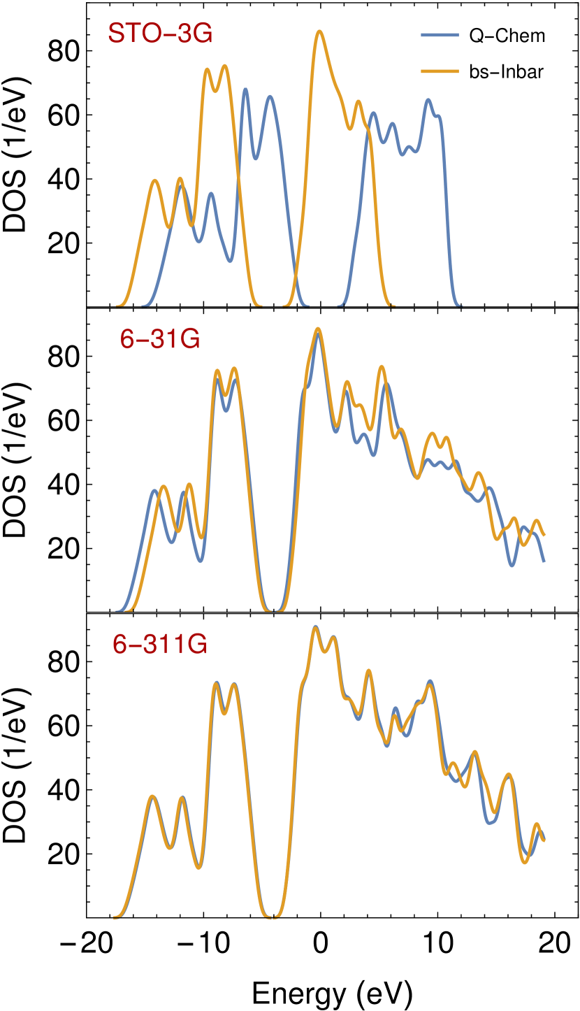
Figure 1: The DOS as a function of energy for a hydrogen-saturated silicon cluster ($\text{Si}_{87}\text{H}_{76}$) calculated using the all-electron Q-CHEM (Shao et al., 2015) and the the bs-Inbar codes. Comparison is made for three standard Gaussian basis-sets as indicated in the panels. We used the local density approximation (LDA) for the exchange-correlation energy. Both calculations plot the DOS of Eq. (13) using $k_{B}T=0.01E_{h}$.

Let us digress a little to explain how we make the calculations, presented in this review, that enable us to study the properties of sDFT and compare them to deterministic calculations. The code we have written for that purpose is called bs-Inbar , and implements both the deterministic Kohn-Sham DFT approach described in the present and previous sections as well as the stochastic DFT to be discussed below. Following previous works (Soler et al., 2002; VandeVondele et al., 2005), we use an auxiliary equally-spaced (grid spacing $\Delta x=0.5a_{0}$) Cartesian grid for calculating the electron-nuclear interaction integrals $V_{\alpha\alpha^{\prime}}^{en}$, the Coulomb repulsion integrals $J_{\alpha\alpha^{\prime}}$, built from the grid vector representing the density $n\left(\boldsymbol{r}\right)$ using fast Fourier transform techniques, and the exchange correlation integrals $V_{\alpha\alpha^{\prime}}^{xc}$. This is the $n\left(\boldsymbol{r}\right)\to\left\{v_{H}\left[n\right]\left(\boldsymbol{r}\right),v_{xc}\left[n\right]\left(\boldsymbol{r}\right)\right\}\to F$ step of Eq. (4). We developed efficient methods to represent the basis functions on the grid to quickly generate molecular orbitals of the type of Eq. (1) on the grid. These techniques are necessary for the step $F\to n\left(\boldsymbol{r}\right)$ of Eq. (17) for generating the density $n\boldsymbol{\left(r\right)}$ from the DM Eq. (16). There are some technical details, such as the effects of core electrons, which cannot be treated efficiently on the grid, and thus are taken into account using norm-conserving pseudopotentials techniques (Troullier and Martins, 1991; Kleinman and Bylander, 1982), and the deleterious Coulomb/Ewald images which are screened out using the method of Ref. Martyna and Tuckerman, 1999. Additional technical elements concerning the bs-Inbar implementation will be presented elsewhere. In Fig. 1 we demonstrate the validity of the deterministic bs-Inbar implementation by comparing its $\text{Si}_{87}\text{H}_{76}$ DOS function to that obtained from the eigenvalues of an all-electron calculation within the same basis-set (using the Q-CHEM program (Shao et al., 2015)). For the largest basis-set (triple zeta 6-311G) the two codes produce almost identical DOS (with small difference at high energies), while for the smallest basis (STO-3G) the all electron result shifts strongly to higher energies. Clearly, the bs-Inbar results are less sensitive to the basis-set, likely due to the use of pseudopotentials instead of treating core electrons explicitly.

Having demonstrated the validity of our deterministic numerical implementation by comparing to deterministic DFT results of Q-CHEM, let us now turn our attention to demonstrating the validity of the sDFT calculation when comparing it to deterministic calculation under the same conditions. In Fig. 2 (top panel) where we plot, for water clusters of three indicated sizes, the energy per electron as a function of $1/I$, where $I$ is the number of random vector $\chi^{\prime}s$ used for the stochastic trace formulas (Eq. (22)-(24)). As the the number of random vectors $I$ grows (and $1/I$ drops) the results converge to the deterministic values (shown in the figure as stars at $1/I=0$). We repeated the calculations 10 times with different random number generator seeds and used the scatter of results for estimating the standard deviation $\sigma$ and the expected value $\mu$ (these are represented, respectively, as error bars and their midpoints in the figure). It is seen that the standard deviation in the energy per particle drops as $I$ increases and in Fig. 3 it is demonstrated that the standard deviation drops as $I^{-1/2}$, in accordance with the central limit theorem. The average values of the energy per particle in Fig. 2 drop steadily towards the converged deterministic values (stars). The fact that the average is always larger than the exact energy, as opposed to fluctuating around it, is a manifestation of a bias $\delta E$ in the method. When $\delta E$ is larger than $\sigma$ it drops in proportion to $I^{-1}$. In subsections (II.3.3)-(II.3.4) we will discuss and explain this behavior.

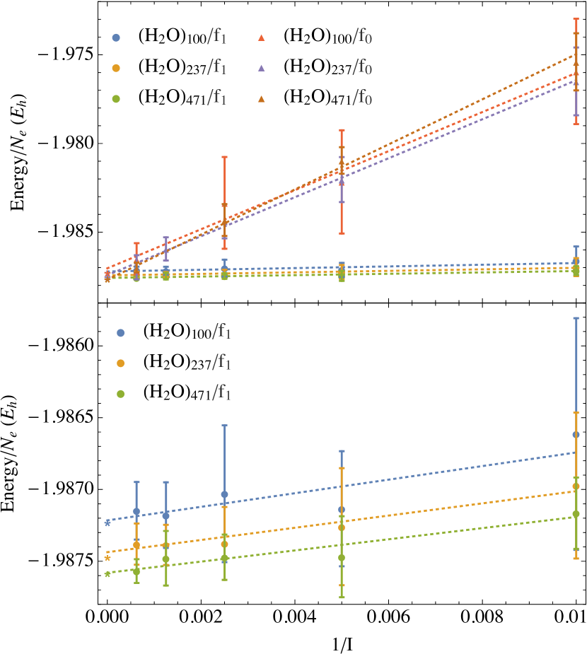
Figure 2: Top panel: The estimate of energy per electron as a function of the inverse number of random vectors ($1/I$) for water molecule clusters of indicated sizes, without fragments ($/f_{0}$) and with fragments (discussed in section (III)) of single $\text{H}_{2}\text{O}$ molecules ($/f_{1}$). The dotted lines are linear fit to the data (weighted by the inverse error bar length). The deterministic results are represented at $1/I=0$ by star symbols. Bottom panel: a zoomed view of the $/f_{1}$ results. These results were calculated using the STO-3G basis-set within the LDA.

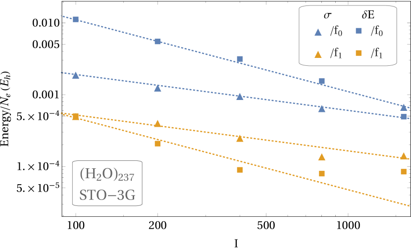
Figure 3: The standard deviation ($\sigma,$circles) and errors ($\delta E$, squares) of the stochastic estimate of the energy per electron as a function of the number of random vectors ($I$) in $\left(\text{H}_{2}\text{O}\right)_{237}$ without fragments ($/f_{0}$, blue) and with $\text{H}_{2}\text{O}$ fragments ($/f_{1}$, yellow, discussed in section (III)) . The dashed lines are best fit functions $\alpha I^{-n}$to the data, where $n=1/2$ for fitting the standard deviations and $n=1$ for the bias. These results were calculated using the STO-3G basis-set within the LDA.

II.3.3 Statistical fluctuations

It is straightforward to show that the variance of the trace formula Eq. (18) is:

$$\Sigma_{M}^{2} \equiv\text{{Var}}\left\{\sum_{\alpha\alpha^{\prime}}^{K}\chi_{\alpha}M_{\alpha\alpha^{\prime}}\chi_{\alpha^{\prime}}\right\}$$ (25)

$$=\frac{1}{2}\sum_{\alpha\neq\alpha^{\prime}}^{K}\left(M_{\alpha\alpha^{\prime}}+M_{\alpha^{\prime}\alpha}\right)^{2}$$

$$=\left(\text{sym}\right)2\sum_{\alpha\neq\alpha^{\prime}}^{K}M_{\alpha\alpha^{\prime}}^{2},$$ (26)

where $\left(\text{sym}\right)$ marks an equality when $M$ is a symmetric matrix. Therefore, from Eq. (15) the variance in the density $\hat{n}\left(\boldsymbol{r}\right)$ is

$$\text{{Var}}_{\text{I}}\left\{\hat{n}\left(\boldsymbol{r}\right)\right\} =\frac{8}{I}\sum_{\alpha\neq\alpha^{\prime}}^{K}\left[\sum_{\beta}^{K}P_{\alpha\beta}\phi_{\beta}\left(\boldsymbol{r}\right)\phi_{\alpha^{\prime}}\left(\boldsymbol{r}\right)\right]^{2}.$$ (27)

The quantity inside the square brackets involves a limited number, independent of system size, of $\alpha^{\prime}$-$\beta$ index pairs $\left[\left(PS\right)_{\alpha\alpha^{\prime}}\right]^{2}$ and since $tr\left[PS\right]=N_{e}$ we can assume that the magnitude of the brackets squared is $O\left(\frac{N_{e}}{K}\right)^{2}$, i.e. independent of system size. Summing over $\alpha$ introduces a system size dependence, hence we conclude that $\text{{Var}}_{\text{I}}\left\{\hat{n}\left(\boldsymbol{r}\right)\right\}$ has magnitude of $O\left(\frac{N_{e}}{I}\right)$. When the system is large enough $P$ becomes sparse and then $\text{{Var}}_{\text{I}}\left(n\left(\boldsymbol{r}\right)\right)$ will tend to become of the magnitude $O\left(\frac{1}{I}\right)$, i.e. system-size independent. The same kind of analysis applies to any single electron observable $\hat{O}$ with sparse matrix representation:

$$\boldsymbol{\text{Var}}_{\text{I}}\left\{\hat{O}\right\}\propto\frac{N_{e}}{I}.$$ (28)

and independent of system size once $P$ localizes. Since intensive properties are obtained by dividing the related extensive properties by $N_{e}$, the standard deviation per electron of intensive properties will evaluate as:

$$\sigma_{\text{intensive}} \propto\frac{\sqrt{\boldsymbol{\text{Var}}_{\text{I}}\left\{\hat{n}\left(\boldsymbol{r}\right)\right\}}}{N_{e}}\propto\frac{1}{\sqrt{IN_{e}}}.$$ (29)

The decay of the sDFT fluctuations with system size, first pointed out in Ref. Baer et al., 2013, is compatible with the fact that fluctuations in intensive variables decay to zero in the thermodynamic limit (Gibbs, 1902). For non-metallic systems $P$ becomes sparse as system size grows. Once this sparsity kicks in, $\sigma_{\text{intensive}}$ is expected to decay as $1/\left(\sqrt{I}N_{e}\right)$. A numerical demonstration of Eq. (29) is given in Fig. 4, for systems of varying numbers $N_{waters}$ of water molecules (all using $I=100$ random vectors $\chi$), where the standard deviation $\sigma$ in the energy per particle (blue triangles) indeed drops with system size roughly as $N_{water}^{-1/2}$.

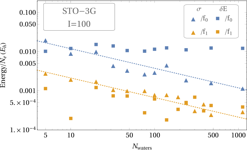
Figure 4: The standard deviation ($\sigma$, triangles) and errors ($\delta E$ squares) of the stochastic estimate of the energy per electron as a function of the number of water molecules $N_{water}$ using no fragments ($/f_{0}$, blue markers) and single water molecule fragments ($/f_{1}$, yellow markers). The dotted lines are $1/\sqrt{N_{water}}$ fits to the $\sigma$ values. These results were calculated using the STO-3G basis-set within the LDA and employed $I=100$ random vectors.

II.3.4 Bias due to nonlinearities

In sDFT, the Hamiltonian $H=S^{-1}F$ is estimated using a random density, and therefore it too, is a random variable with an expected value $\bar{H}=\text{{E}}\left\{H\right\}$ and a fluctuation due to the a covariance matrix $\sigma_{ij;kl}^{2}=\boldsymbol{\text{E}}\left\{H_{ij}H_{kl}\right\}-\bar{H}_{kl}$. Consider an observable $\hat{O}$ with an exact expectation value $\left\langle\hat{O}\right\rangle_{\bar{H}}=\text{Tr}\left(f\left(\bar{H};T,\mu\right)S^{-1}O\right)$ (Eqs. (8) and (21)). We note, that even when $\bar{H}$ is the exact (deterministic) Hamiltonian, the expectation values $\left\langle\hat{O}\right\rangle_{H}$ will not average to the exact value $\left\langle\hat{O}\right\rangle_{\bar{H}}$, simply because the function of the average of a random variable is distinct or “biased” from the average of the function: $\text{{E}}\left\{\left\langle\hat{O}\right\rangle_{H}\right\}\neq\left\langle\hat{O}\right\rangle_{\bar{H}}$. Clearly, the extent of this bias stems from the how $\boldsymbol{\text{E}}\left\{f\left(H;T,\mu\right)\right\}$ deviates from $f\left(\boldsymbol{\text{E}}\left\{H\right\};T,\mu\right)$ and using Taylor’s theorem this can be estimated as

$$\text{{E}}\left\{f\left(H;T,\mu\right)\right\} -f\left(\bar{H};T,\mu\right)=$$ (30)

$$\frac{1}{2}\sum_{i,j,k,l} \sigma_{ij;kl}^{2}\frac{\partial}{\partial H_{ij}}\frac{\partial}{\partial H_{kl}}f\left(\bar{H};T,\mu\right).$$

There are three lessons from this analysis: 1) all expectation values $\left\langle\hat{O}\right\rangle$ based on $I$ random vectors in the sDFT method suffer a bias $\delta\left\langle\hat{O}\right\rangle\propto\text{coVar}_{\text{I}}\left\{H\right\}\propto\text{Var}_{\text{I}}\left\{\hat{O}\right\}$ ; 2) from Eq. (28) this bias in the intensive value $\left\langle\hat{O}\right\rangle/N_{e}$ is proportional to $I^{-1}$ but independent from system size; and lastly: the double derivative of $f$ on the right hand side of Eq. (30) (called the “Hessian”) is related in a complicated way to the curvature $f^{\prime\prime}\left(\varepsilon;T,\mu\right)$ of the Fermi-Dirac function. This curvature is practically zero for almost all $\varepsilon$ except near $\varepsilon\approx\mu\pm k_{B}T$, and for sufficiently small temperatures, the large Fermi-Dirac curvature regions are safely tucked into the HOMO-LUMO gap, so that indeed the bias can be small.

Summarizing, we find the following trends in the SEs of intensive quantities:

$$\sigma_{\text{intensive}} \propto\left(\frac{1}{N_{e}I}\right)^{1/2},$$ (31)

$$\delta_{\text{intensive}} \propto\frac{1}{I}.$$ (32)

Numerical demonstrations of Eq. (32) are given in Fig. 3 (blue squares) where the bias $\delta E/N_{e}$ is seen to drop as $I^{-1}$ and in Fig. 4 (blue squares) where the bias is seen to be independent of the system size.

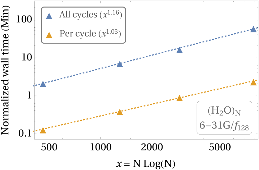
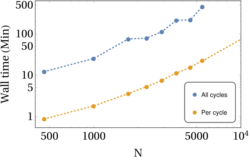
Figure 5: The timing of DFT calculations of $\left(\text{H}_{2}\text{O}\right)_{N}$ water clusters using the 6-31G basis-set within the LDA. Left panel: The sDFT wall time as function of $x=N\log N$ normalized to one random orbital per thread for a full SCF calculation (blue symbols) and for a single SCF cycle (orange symbols). Dashed lines are functions $t=Ax^{n}$, where $n$ is best-fitted to the data and shown in the legend. Right panel: Wall time of a conventional SCF calculation (using Q-CHEM (Shao et al., 2015)), performed on a single node, as a function of $N$ for a full SCF calculation (blue symbols) and for a single SCF cycle (orange symbols). The Calculations were run on an Intel Xeon CPU E3-1230 v5 @ 3.40GHz 64 GB RAM (without Infiniband networking). Each processor supports 8 threads. The sDFT results were calculated with 800 random vectors and fragments of a representative size of 128 water molecules (denoted $/f_{128}$).

II.3.5 Scaling and scalability

In the left panel of Fig. 5 we show, using a series of water clusters how wall times scale as a function of system size for the sDFT calculation. Because the evaluation of the Hartree potential is made with fast Fourier transforms, the effort is expected to scale as $x=N\log N$ where $N$ indicates the number of water molecules. When considering a single SCF iteration we find this near-linear-scaling as expected. When considering the entire calculation until SCF convergence (which is achieved when the change in the total energy per electron is smaller than $10^{-5}E_{h}$), we find the number of SCF iterations growing gently with system size and the scaling seems to be near $O\left(x^{1.16}\right)$.

As demonstrated in Fig. 6, we see excellent scalability with number of processors with a mere 8% decrease from the ideal speedup when the number of cores was increased by a factor of 8. This is a result of assigning to each thread a smaller number of random vectors. Ideal wall times are achieved when the there is but one stochastic orbital per thread . For the systems studied Fig. 5 it is an hour for a full SCF calculation of the water 1100 system (ca. 9000 electrons, 13000 orbitals).

Under these conditions, the sDFT wall-times can be significantly lower than those of “conventional” basis-set DFT calculations, as shown in the right panel of Fig. 5. This happens despite the fact that the program used, Q-CHEM, was remarkably still showing quadratic scaling since the cubic scaling component was not yet dominant.

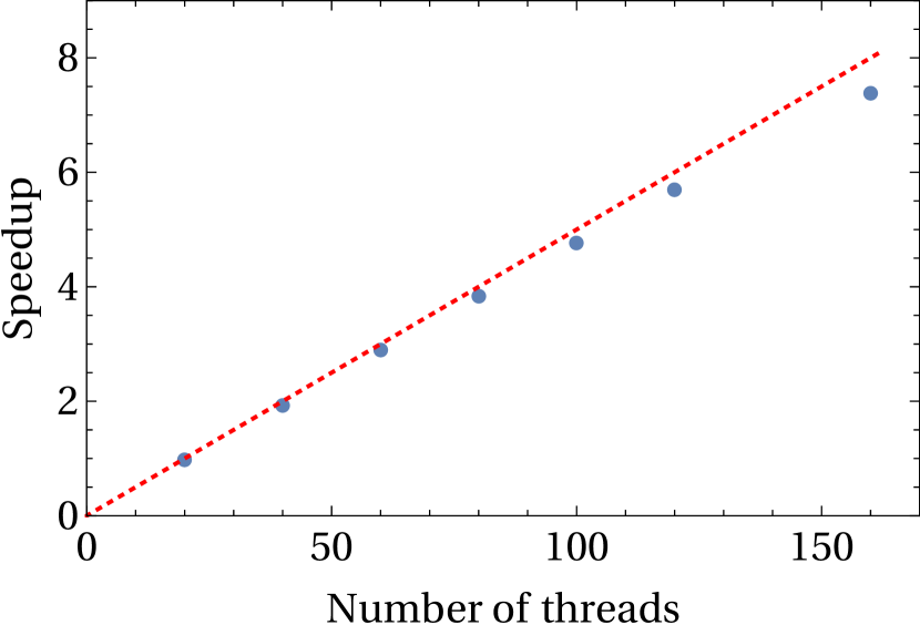
Figure 6: Scalability plot of the calculation, showing the speedup as a function of the number of threads used when calculating a SCF iteration of $\left(\text{H}_{2}\text{O}\right)_{1120}$ (at the 6-31G basis-set level within LDA) using a total of 2400 random vectors. Calculations were performed on several 2.30GHz Intel Xeon E5-2650 v3 with 252 GB and Infiniband networking.

III Embedded fragments method

III.1 Theory

The notion of fragments, developed first in Ref. Neuhauser et al., 2014 was to break up the system into disjoint pieces called fragments labeled by the index $f$, and for each fragment compute a DM $P^{f}$, such that to a good approximation we can write:

$$P\approx\sum_{f}P^{f}.$$ (33)

Clearly, the coherences between different fragments are also missing from $\sum_{f}P^{f}$ and these too are assumed small but not totally negligible. From Eq. (9), the expectation value of an arbitrary one-electron operator $\hat{O}$ can be expressed as a contribution of two terms, $\left\langle\hat{O}\right\rangle=2\text{Tr}\left[\sum_{f}P^{f}O\right]+2\text{Tr}\left[\left(P-\sum_{f}P^{f}\right)O\right]$, where the first is the “fragment expected value” and the second is a correction, expressed as a small trace to be evaluated using the stochastic trace formula. Applying the stochastic trace formula to just a small trace obviously lowers the SEs when compared to using it for a full trace.

Ref. Neuhauser et al., 2014 considered two types of fragmentation procedures. The first was to used natural fragments which could just be considered separately, for example, a single water molecule in a water cluster or a single $\text{C}_{60}$ molecule in a cluster of $\text{C}_{60}$’s. Since the molecules are not covalently bonded they are weakly interacting and Eq. (33) is expected to be satisfied to a good degree (however, adjacent water molecules can interact via hydrogen bonds and this may reduce the efficacy of the single-molecule fragments, as discussed below).

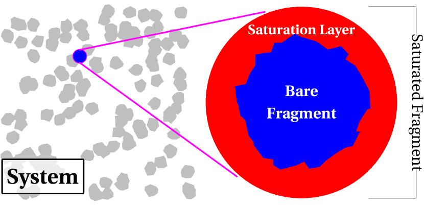
Figure 7: A schematic depiction of a bare fragment (blue region) as a localized set of atoms or molecules within the large system. The fragment is first saturated by coating it with capping atoms (red region), its saturated-DM is calculated using a deterministic DFT calculation, from which a bare DM $P^{f}$ is is “carved” out by an algebraic procedure.

The efficiency of the fragments depends entirely on the closeness of the approximation in Eq. (33) and therefore significant effort has to go to developing techniques for constructing fragments. One can probably make good use of the experience gained by the biological and materials embedding methods (Barone et al., 2010; van der Kamp and Mulholland, 2013; Sabin et al., 2010; Huang and Carter, 2011; Lan et al., 2015; Ghosh et al., 2010; Elliott et al., 2010).

The notion of saturated fragments was developed further in Ref. Arnon et al., 2017 and used in silicon clusters where covalent bonds were cut when forming the bare fragment. The dangling bonds on the surface of the bare fragments were then saturated with foreign H or Si atoms. This produced a saturated fragment (see Fig. 7) and a special algebraic technique was developed for carving out the bare fragment DM $P^{f}$. The results facilitated what seems to be nearly unbiased force evaluations for the atoms in large nanocrystals, with the structure studied using Langevin molecular dynamics.

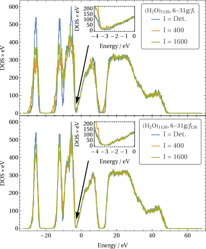
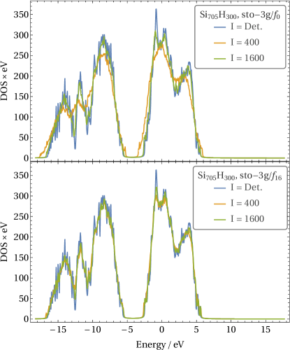
Figure 8: Left panels: The LDA DOS of a cluster of 1120 water molecules using the 6-31G basis-set computed with $I=400$ and $I=1600$ random vectors and using single-molecule fragments ($/f_{1}$ top panel) and 128 molecule fragments ($/f_{128}$ bottom left panel). The insets zoom on the region of the band gap. Right panels: The LDA DOS of $\text{Si}_{705}\text{H}_{300}$, a hydrogen-terminated silicon nanocrystal, using the STO-3G basis-set computed with $I=400$ and $I=1600$ random vectors and using no fragments ($/f_{0}$ top panel) and 16 atom fragments ($/f_{16}$ bottom panel). In all panels the results are compared to deterministic calculations under the same conditions.

III.2 Efficiency of the embedded fragments

To asses the utility of fragments that do not strictly require saturation, such as water fragments in water clusters, consider first Fig. 2, where we compare the energy per particle of $\left(\text{H}_{2}\text{O}\right)_{n}$, with $n=100$, $237$ and $471$, estimated using sDFT with no fragments (denoted $/f_{0}$) and using fragments of just one water molecule ($/f_{1})$. It is seen that there is a dramatic decrease in the the standard deviation and in the bias. In Fig. 3 we study in more detail $\left(\text{H}_{2}\text{O}\right)_{n}$, finding that with no fragments we are in a bias dominated regime while the use of fragments allows us to move to a regime controlled by fluctuations. Evidently, in the latter case, the large fluctuations mask the linear decrease of the bias with $1/I$, which was so clearly visible in the former one. In Fig. 4, we study the SEs as a function of system size $N$, comparing the calculations with and without fragments. We see that while fragments help reducing SEs, they do not change the fact that the bias is largely independent of $N$.

The use of fragments greatly benefits other types of sDFT observables. Consider, for example, the density of states function $\rho_{e}\left(E\right)$ of water (Neuhauser et al., 2014). In the left panels of Fig. 8 we plot the DOS for a $\left(\text{H}_{2}\text{O}\right)_{1120}$ cluster described using the 6-31G basis-set comparing to the deterministic result under an identical setup. We see in the top left panel, that by using $I=400$ random vectors and small single-molecule fragments ($/f_{1}$), the sDFT DOS generally follows that of the exact calculation quite closely. However, a zoom into the frontier orbital gap shows, that even though the stochastic-based calculation exhibits, as it should, a very low DOS in the frontier gap region, there is clearly room for further improvement, since the gap is not sufficiently-well described. Increasing the number of random vectors used from $I=400$ to $I=1600$ improves the overall accuracy but increasing the fragment size to 128 water molecules ($/f_{128}$) is even more advantageous, as can be seen in the lower left panel of the figure. It is evident from this description that it is crucial to develop methods that enable better fragments (in the sense that the approximation in Eq. (33) is as tight as possible). Despite the obvious utility of the fragments for the water cluster systems, there is a need to reach quite large fragments for high accuracy. Perhaps this is due to the fact that we do not saturate the bare fragments with their neighboring molecules, as first suggested in recent unpublished work (Ming et al., 2018). Future work will test this hypothesis.

Finally we also show in Fig. 8 (right panels) the effect of fragments on the DOS of a large silicon cluster. Here, we must use saturated fragments, as was done in Ref. Arnon et al., 2017. The density of states, compared to a deterministic calculation is again greatly improved when fragments of size 16 silicon atoms are used (bottom left panel).

III.3 Localized energy changes

So far, we have dealt with two types of observables: intensive properties (such as energy per electron) which is a highly averaged quantity, and density of states which, due to the tall number of levels in large systems can be smeared, i.e. locally average, with little loss of essential accuracy. We now demonstrate the possibility of calculating forces on a small atom or molecule within the large system, using stochastic DFT. Previous works concerning this issue (Baer et al., 2013; Arnon et al., 2017) demonstrated that the Hellman-Feynman force $F^{a}=-\int n\left(\boldsymbol{r}\right)\frac{\partial}{\partial R^{a}}v_{eN}\left(\boldsymbol{r}\right)d\boldsymbol{r}+\sum_{a\neq a}\frac{Z_{a}Z_{a^{\prime}}\left(\boldsymbol{R}^{a}-\boldsymbol{R}^{b}\right)}{\left|\boldsymbol{R}^{a}-\boldsymbol{R}^{b}\right|^{3}}$ involves a controlled variance and small bias.

Here we consider a related but different question, the possibility of systematically reducing the bias in forces on nuclei within a localized region of interest in a large system. This is useful when modeling reactions in biomolecular systems, as often done using the QM/MM approach, where quantum chemistry forces are used for simulating chemical reactions and other electronic processes (charge transfer or excitation) while force fields are used for the rest of the system (Cho et al., 2005; Svozil and Jungwirth, 2006; Lin and Truhlar, 2007; Sharir-Ivry et al., 2008; Sabin et al., 2010; Barone et al., 2010; van der Kamp and Mulholland, 2013).

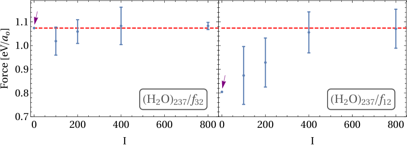
Figure 9: The force on a marked water molecule in $\left(\text{H}_{2}\text{O}\right)_{237}$ (red dashed line is the deterministic DFT value) calculated as $-\delta E/\delta x$ where $\delta E$ is the energy difference between two positions of the molecule displaced by a distance $\delta x=0.05a_{0}$. On the left (right) panel we present $/f_{12}$ ($/f_{32}$) results. The arrow points to the force $F\left(I=0\right)$ (the deterministic force on the molecule when in the parent fragment). The “error bars” are 95% confidence intervals for $\text{{E}}\left\{F\left(I\right)\right\}$. These results were calculated using the STO-3G basis-set within the LDA.

For this, we take a fragment which encapsulates the region of interest and “embed” it into the system using sDFT. We study such a process in Fig. 9 where the force $F$ exerted on a certain, marked, water molecule in a larger $\left(\text{H}_{2}\text{O}\right)_{237}$ cluster is calculated, first by deterministic DFT (shown as a dashed red line in the figure) and then by sDFT as a function of the number of random vectors $I$ ($F\left(I\right)$), using two types of fragment sizes: 12-molecule fragments ($/f_{12}$), on the left, and larger 32-molecule fragments ($/f_{32})$ on the right. We note, that $F\left(I=0\right)$ is the deterministic force felt by the molecule in its parent fragment. In the right panel we show the case of a parent fragment which fully encloses the marked molecule. At $I=0$ the force is already very close to the deterministic value, indicating $\sum_{f}P_{f}$ is an excellent approximation for $P$. When embedded by $I>0$ stochastic iterations, we find that fluctuations are introduced, but the error bars (marking 95% chance that $\text{{E}}\left\{F\left(I\right)\right\}$ always include the exact value) indicate a small bias (such that the error is not dominated by the bias). If we repeat this calculation, but use small fragments which do not encapsulate the marked molecule, the $F\left(I=0\right)$ is very different from the deterministic exact force ($\sum_{f}P_{f}$ is a deficient approximation for $P$). When embedded by $I>0$ stochastic iterations, the bias is gradually removed as $I$ grows, in accordance with the steady diminishing of the bias discussed in subsection II.3.4.

We may conclude from this computational experiment that sDFT may be especially useful for studying chemical processes in small subsystems which can be encapsulated in fragments. Without using fragments, this is also possible an increase in the number of samplings $I$ needs to be employed in order to remove the bias.

IV Summary and Discussion

The sDFT approach has been used in various means and for a selection of applications (Baer et al., 2013; Neuhauser et al., 2014; Arnon et al., 2017; Cytter et al., 2018; Neuhauser et al., 2015; Ming et al., 2018). The common thread for all the previous sDFT works was its formulation using an orthogonal basis (grids or plane-waves representation). In this review, we have focused on studying sDFT in the perspective of a local non-orthogonal basis-set. One advantage of the localized basis-set method is that even for large systems the deterministic calculation can still be performed allowing to study in detail errors and their dependence on system size.

The sDFT theory was described using three stages, starting from the standard basis-set formulation of DFT, leading to cubic scaling. Next, we developed a deterministic trace-based calculation, exploiting the sparsity of the Fock and overlap matrices, which lead to a quadratic approach but remained numerically accurate. Finally, came the sDFT which uses stochastic sampling to evaluate the trace-based calculations, thereby lowering the scaling to linear. The price to pay is the introduction of statistical errors, which one can mitigate by increasing the sampling rate. In order to study and demonstrate the sDFT properties, we developed a basis-set DFT approach using an auxiliary grid for constructing the Hartree and exchange-correlation matrices. Based on this code we also developed the stochastic sDFT implementation. We also developed a basis-set-based fragment method and tested its utility

Using the code, we analyzed the statistical errors associated with the stochastic calculations and their dependence on the number of stochastic samples $I$, the system size, $N$ (one can take the number of electrons $N_{e}$ or the basis-set size $K$ as $N$), and the fragment size. As in previous sDFT papers, the results demonstrated a $I^{-1/2}$ and $N^{-1/2}$ dependence of the statistical fluctuations. Furthermore, we were able to explore the nature of the systematic errors in the sDFT calculation. The bias errors in stochastic methods, have been discussed before in (Cytter et al., 2018; Neuhauser et al., 2017). In sDFT we show that they do not grow with system size and that they decay as $I^{-1}$. We also developed an analytical model to explain these observations.

It has also been shown that using fragments the noise in the results can be significantly reduced reaching a regime where the statistical fluctuations are the dominating contributions to the error (rather than the bias). These conclusions are in line with previous studies (Neuhauser et al., 2014; Arnon et al., 2017; Chen et al., 2018), By implementing the fragments we were able to calculate other observables (such as the density of states, or forces) in a much more accurate fashion for a very similar cost.

We demonstrated that our sDFT implementation displays system-size linear-scaling CPU time (Figure 5) and that it is efficacious in parallel architectures (Figure 6). Indeed, it seems to reach its full utility in CPU-abundant architectures, suggesting it may be suitable for Exascale computing.

Future work in the sDFT implementation is required for speeding up the calculations on each node, this can be achieved by shared-memory or GPU parallelization. Further development is also needed for improved fragments which will reduce the variance and bias errors as well as reduce the number of SCF iterations. Finally, as mentioned above, using the sDFT code to drive a Langevin sampling of the nuclear configurations (Arnon et al., 2017) will allow us to compute observables related to the thermal-nuclear structure of the molecular systems.