Differential Dynamic Programming for Nonlinear Dynamic Games

Abstract

Dynamic games arise when multiple agents with differing objectives choose control inputs to a dynamic system. Dynamic games model a wide variety of applications in economics, defense, and energy systems. However, compared to single-agent control problems, the computational methods for dynamic games are relatively limited. As in the single-agent case, only very specialized dynamic games can be solved exactly, and so approximation algorithms are required. This paper extends the differential dynamic programming algorithm from single-agent control to the case of non-zero sum full-information dynamic games. The method works by computing quadratic approximations to the dynamic programming equations. The approximation results in static quadratic games which are solved recursively. Convergence is proved by showing that the algorithm iterates sufficiently close to iterates of Newton’s method to inherit its convergence properties. A numerical example is provided.

I INTRODUCTION

Dynamic games arise when multiple agents with differing objectives act upon a dynamic system. In contrast, optimal control can be viewed as the specialization of dynamic games to the case of a single agent. Dynamic games have many applications including pursuit-evasion [1], active-defense [2, 3], economics [4] and the smart grid [5]. Despite a wide array of applications, the computational methods for dynamic games are considerably less developed than the single-agent case of optimal control.

This paper shows how the differential dynamic programming (DDP) method from optimal control [6] extends to discrete-time non-zero sum dynamic games. Closely related works from [7, 8] focus on the case of zero-sum dynamic games. Classical differential dynamic programming operates by iteratively solving quadratic approximations to the Bellman equation from optimal control. Our method applies similar methods to the generalization of the Bellman equation for dynamic games [9]. Here, at each stage, the algorithm solves a static game formed by taking quadratic approximations to the value function of each agent. We show that the algorithm converges quadratically in the neighborhood of a strict Nash equilibrium. To prove convergence, we extend arguments from [10], which relate DDP iterates to those of Newton’s method, to the case of dynamic games. In particular, we extend the recursive solution for Newton’s method [11] to dynamic games, and demonstrate that the solutions produced Newton’s method and the DDP method are close.

I-A Related Work

A great deal of work on algorithmic solutions to dynamic games has been done. This subsection reviews related work which is a bit more removed from the closer references described above. As we will see, most works solve somewhat different problems compared to the current paper.

Methods for finding Nash equilibria via extremum seeking were presented in [12, 13, 14]. In particular, the controllers drive the states of a dynamic system to Nash equilibria of static games. A related method for linear quadratic games was presented in [15]. For these works, each agent only requires measurements of its own cost. However, it is limited to finding equilibria in steady state. Our method requires each agent to have explicit model information, but gives equilibria over finite horizons. This is particularly important for games in which trajectories from initial to final states are desired.

Several works focus on the solution to dynamic potential games. Potential games are more tractable than general dynamic games, as they can be solved using methods from single-agent optimal control [16, 17, 18, 19, 20, 21]. However, potential games satisfy restrictive symmetry conditions. In particular, the assumption precludes interesting applications with heterogeneous agents.

I-B Paper Outline

The general problem is formulated in Section II. The algorithm is described in Section III and the convergence proof is sketched in Section IV. A numerical example is described in V. Conclusions and future directions are discussed in VI while the proof details are given in the appendix.

II DETERMINISTIC NONLINEAR DYNAMIC GAME PROBLEM

In this section, we introduce deterministic finite-horizon nonlinear game problem, the notations for the paper, the solution concept and convergence criterion of our proposed method.

The main problem of interest is a deterministic full-information dynamic game of the form below.

Problem 1

Nonlinear dynamic game
Each player tries to minimize their own cost

$$J_{n}(u)=\sum_{k=0}^{T}c_{n,k}(x_{k},u_{:,k})$$ (1)

Subject to constraints

$$x_{k+1}=f_{k}(x_{k},u_{:,k})$$ (2a)

$$x_{0}\textrm{ is fixed.}$$ (2b)

Here, the state of the system at time $k$ is denoted by $x_{k}\in\mathbb{R}^{n_{x}}$.

Player $n$’s input at time $k$ is given by $u_{n,k}\in\mathbb{R}^{n_{u_{n}}}$. The vector of all player actions at time $k$ is denoted by: $u_{:,k}=[u_{1,k}^{\top},u_{2,k}^{\top},\ldots,u_{N,k}^{\top}]^{\top}\in\mathbb{R}^{n_{u}}$. The cost for player $n$ at time $k$ is $c_{n,k}(x_{k},u_{:,k})$. This encodes the fact that the costs for each player can depend on the actions of all the players.

In later analysis, some other notation will be helpful. The vector player $n$’s actions over all time is denoted by $u_{n,:}=[u_{n,0}^{\top},u_{n,1}^{\top},\ldots,u_{n,T}^{\top}]^{\top}$. The vector of all actions other than those of player $n$ is denoted by $u_{-n,:}=[u_{1,:}^{\top},\ldots,u_{n-1,:}^{\top},u_{n+1,:}^{\top},\ldots,u_{N,:}^{\top}]^{\top}$. The vector of all states is denoted by $x=[x_{0}^{\top},x_{1}^{\top},\ldots,x_{T}^{\top}]^{\top}$ while the vector of all inputs is given by $u=[u_{1,:}^{\top},u_{N,:}^{\top},\ldots,u_{N,:}^{\top}]^{\top}$.

Note that since the initial state is fixed and the dynamics are deterministic, the costs for each player can be expressed as functions of the vector of actions, $J_{n}(u)$.

A local Nash equilibrium for problem 1 is a set of inputs $u^{\star}$ such that

$$J_{n}(u_{n,:},u_{-n,:}^{\star})\geq J_{n}(u^{\star}),\ n=1,2,\ldots,N$$ (3)

for all $u_{n,:}$ in a neighborhood of $u_{n,:}^{\star}$. In the context of dynamic games, this correponds to an open-loop, local Nash equilibrium [9]. The equilibrium is called a strict local Nash equilibrium if the inequality in (3) is strict for all $u_{n,:}\neq u_{n,:}^{\star}$ in a neighborhood of $u_{n,:}^{\star}$.

In this paper, we focus on computing Nash equilibria by solving the following necessary conditions for local Nash equilibria:

Problem 2

Necessary conditions

$$\frac{\partial J_{n}}{\partial u_{n,:}}=0$$ (4)

for $n=1,\ldots,N$.

For convenient notation, we stack all of the gradient vectors from (4) into a single vector:

$$\mathcal{J}(u)=\begin{bmatrix}\frac{\partial J_{1}}{\partial u_{1,:}}&\frac{\partial J_{2}}{\partial u_{2,:}}&\cdots&\frac{\partial J_{N}}{\partial u_{N,:}}\end{bmatrix}^{\top}.$$ (5)

Thus, the necessary condition is equivalent to $\mathcal{J}(u)=0$. Such conditions arise in works such as [22, 23].

We will present a method for solving these necessary conditions for a local Nash equilibrium via differential dynamic programming (DDP). In principle, an input vector satisfying the necessary conditions $\mathcal{J}(u)=0$ could be found via Newton’s method. Similar to the single-player case from [10], we analyze the convergence properties of DDP by proving that its solution is close to that computed by Newton’s method.

To guarantee convergence, we assume that $\mathcal{J}(u)$ satisfies the smoothness and non-degeneracy conditions required by Newton’s method [24]. For smoothness, we assume that $\mathcal{J}(u)$ is differentiable with locally Lipschitz derivatives. For non-degeneracy, we assume that $\frac{\partial\mathcal{J}(u^{*})}{\partial u}$ is invertible. A sufficient condition for the smoothness assumptions is that the functions $f_{k}$ and $c_{n,k}$ are twice continuously differentiable with Lipschitz second derivatives. In our DDP solution, we will solve a sequence of stage-wise quadratic games. As we will see, a sufficient condition for invertibility of $\frac{\partial\mathcal{J}(u^{*})}{\partial u}$ is the unique solvability of the stage-wise games near the equilibrium.

III Differential Dynamic Programming Algorithm

This section describes the differential dynamic programming algorithm for dynamic games of the form in Problem 1. Subsection III-A gives a high-level description of the algorithm, while Subsection III-B describes the explicit matrix calculations used in algorithm.

III-A Algorithm Overview

The equilibrium solution to the general dynamic game can be characterized by the Bellman recursion:

$$V_{n,T+1}^{\star}(x_{T+1}) =0$$ (6a)

$$Q_{n,k}^{\star}(x_{k},u_{:,k}) =c_{n,k}(x_{k},u_{:,k})+V_{n,k+1}^{\star}(f_{k}(x_{k},u_{:,k}))$$ (6b)

$$V_{n,k}^{\star}(x_{k}) =\min_{u_{n,k}}Q_{n,k}^{\star}(x_{k},u_{:,k}).$$ (6c)

In particular, if a solution to the Bellman recursion is found, the corresponding optimal strategy for player $n$ at time $k$ would be the $u_{n,k}$ which minimizes $Q_{n,k}^{\star}(x_{k},u_{:,k})$. Note that (6c) defines a static game with respect to the $u_{:,k}$ variable at step $k$.

The idea of the differentiable dynamic programming (DDP) is to maintain quadratic approximations of $V_{n,k}^{*}$ and $Q_{n,k}^{*}$ denoted by $\tilde{V}_{n,k}$ and $\tilde{Q}_{n,k}$, respectively.

We need some notation for our approximations. For a scalar-valued function, $h(z)$, we denote the quadratic approximation near $\bar{z}$ by:

$$\textrm{quad}(h(z))_{\bar{z}}= \frac{1}{2}\begin{bmatrix}1\\ \delta z\end{bmatrix}^{\top}\begin{bmatrix}2h(\bar{z})&\frac{\partial h(\bar{z})}{\partial z}\\ \frac{\partial h(\bar{z})}{\partial z}^{\top}&\frac{\partial^{2}h(\bar{z})}{\partial z^{2}}\end{bmatrix}\begin{bmatrix}1\\ \delta z\end{bmatrix}$$ (7a)

$$\delta z= z-\bar{z}.$$ (7b)

If $h:\mathbb{R}^{n}\to\mathbb{R}^{m}$ we form the quadratic approximation by stacking all of the quadratic approximations of the entries:

$$\textrm{quad}(h(z))_{\bar{z}}=[\textrm{quad}(h_{1}(z))_{\bar{z}},\ldots,\textrm{quad}(h_{m}(z))_{\bar{z}}]^{\top}$$ (8)

Let

$$z_{k}=\begin{bmatrix}x_{k}\\ u_{:,k}\end{bmatrix}$$ (9)

and let $\bar{x}_{k}$ and $\bar{u}_{:,k}$ be a trajectory of states and actions satisfying the dynamic equations from (2). The approximate Bellman recursion around this trajectory is given by:

$$\tilde{V}_{n,T+1}(x_{T+1}) =0$$ (10a)

$$\tilde{Q}_{n,k}(z_{k}) =\textrm{quad}(c_{n,k}(z_{k})+\tilde{V}_{n,k+1}(f_{k}(z_{k})))_{\bar{z}_{k}}$$ (10b)

$$\tilde{V}_{n,k}(x_{k}) =\min_{u_{n,k}}\tilde{Q}_{n,k}(x_{k},u_{:,k}).$$ (10c)

Note that (10c) is now a quadratic game in the $u_{:,k}$ variables which has unique and ready solution [9]. Recall the $\mathcal{J}(u)$ function defined in (5). A sufficient condition for solvability of these games is given in terms of $\mathcal{J}(u)$ is given in the following lemma. Its proof is in Appendix A-D.

Lemma 1

If $\frac{\partial\mathcal{J}(\bar{u})}{\partial u}$ is invertible, the game defined by (10c) has a unique solution of the form:

$$u_{:,k}=\bar{u}_{:,k}+\tilde{K}_{k}\delta x_{k}+\tilde{s}_{k}.$$ (11)

In the notation defined above, we have that $\delta x_{k}=x_{k}-\bar{x}_{k}$. Note that if $\frac{\partial\mathcal{J}(u^{\star})}{\partial u}$ is invertible, then $\frac{\partial\mathcal{J}(\bar{u})}{\partial u}$ is invertible for all $\bar{u}$ in a neighborhood of $u^{\star}$.

Here we provide the DDP algorithm for applying DDP game solution in pseudo code.

Algorithm 1 Differential Dynamic Programming for Nonlinear Dynamic Games

Generate an initial trajectory $\bar{x},\bar{u}$

loop

     Backward Pass:

     Perform the approximate Bellman recursion from (10)

     Compute $\tilde{K}_{k}$ and $\tilde{s}_{k}$ from (11).

     Forward Pass:

     Generate a new trajectory using the affine policy defined by $\tilde{K}_{k},\tilde{s}_{k}$

end loop

III-B Implementation Details

All of the operations in the backwards pass of the DDP algorithm, Algorithm 1, can be expressed more explicitly in terms of matrices.

To construct the required matrices, we define the following approximation terms:

$$A_{k}=\frac{\partial f_{k}(x_{k},u_{:,k})}{\partial x_{k}}\Big{|}_{\bar{u}},\quad B_{k}=\frac{\partial f_{k}(x_{k},u_{:,k})}{\partial u_{:,k}}\Big{|}_{\bar{u}}$$ (12a)

$$G_{k}^{l}=\begin{bmatrix}\frac{\partial^{2}f^{l}_{k}}{\partial x_{k}^{2}}&\frac{\partial^{2}f^{l}_{k}}{\partial x_{k}\partial u_{:,k}}\\ \frac{\partial^{2}f^{l}_{k}}{\partial u_{:,k}\partial x_{k}}&\frac{\partial^{2}f^{l}_{k}}{\partial u_{:,k}^{2}}\end{bmatrix}\Bigg{|}_{\bar{u}},\ l=1,2,\ldots,n_{x}$$ (12b)

$$R_{k}(\delta x_{k},\delta u_{:,k})=\begin{bmatrix}\begin{bmatrix}\delta x_{k}\\ \delta u_{:,k}\end{bmatrix}^{T}G_{k}^{0}\begin{bmatrix}\delta x_{k}\\ \delta u_{:,k}\end{bmatrix}\\ \begin{bmatrix}\delta x_{k}\\ \delta u_{:,k}\end{bmatrix}^{T}G_{k}^{1}\begin{bmatrix}\delta x_{k}\\ \delta u_{:,k}\end{bmatrix}\\ \vdots\\ \begin{bmatrix}\delta x_{k}\\ \delta u_{:,k}\end{bmatrix}^{T}G_{k}^{n_{x}}\begin{bmatrix}\delta x_{k}\\ \delta u_{:,k}\end{bmatrix}\end{bmatrix}$$ (12c)

$$M_{n,k} =\left.\begin{bmatrix}2c_{n,k}&\frac{\partial c_{n,k}}{\partial x_{k}}&\frac{\partial c_{n,k}}{\partial u_{:,k}}\\ \frac{\partial c_{n,k}}{\partial x_{k}}^{\top}&\frac{\partial^{2}c_{n,k}}{\partial x_{k}^{2}}&\frac{\partial^{2}c_{n,k}}{\partial x_{k}\partial u_{:,k}}\\ \frac{\partial c_{n,k}}{\partial u_{:,k}}^{\top}&\frac{\partial^{2}c_{n,k}}{\partial u_{:,k}\partial x_{k}}&\frac{\partial^{2}c_{n,k}}{\partial u_{:,k}^{2}}\end{bmatrix}\right\rvert_{\bar{u}}$$ (12d)

$$=\begin{bmatrix}M_{n,k}^{11}&M_{n,k}^{1x}&M_{n,k}^{1u}\\ M_{n,k}^{x1}&M_{n,k}^{xx}&M_{n,k}^{xu}\\ M_{n,k}^{u1}&M_{n,k}^{ux}&M_{n,k}^{uu}\end{bmatrix}.$$

Using the notation from (7), (8) and (9), the second-order approximations of the dynamics and cost are given by:

$$\textrm{quad}(f_{k}(z_{k}))_{\bar{z}_{k}}=f_{k}(\bar{z}_{k})+A_{k}\delta x_{k}+B_{k}\delta u_{:,k}+R_{k}(\delta z_{k})$$ (13a)

$$\textrm{quad}(c_{n,k}(z_{k}))_{\bar{z}_{k}}=\begin{bmatrix}1\\ \delta z_{k}\end{bmatrix}^{\top}M_{n,k}\begin{bmatrix}1\\ \delta z_{k}\end{bmatrix}.$$ (13b)

By construction $\tilde{V}_{n,k}(x_{k})$ and $\tilde{Q}_{n,k}(x_{k},u_{:,k})$ are quadratic, and so there must be matrices $\tilde{S}_{n,k}$ and $\tilde{\Gamma}_{n,k}$ such that

$$\tilde{V}_{n,k}(x_{k}) =\frac{1}{2}\begin{bmatrix}1\\ \delta x_{k}\\ \end{bmatrix}^{\top}\begin{bmatrix}\tilde{S}_{n,k}^{11}&\tilde{S}_{n,k}^{1x}\\ \tilde{S}_{n,k}^{x1}&\tilde{S}_{n,k}^{xx}\end{bmatrix}\begin{bmatrix}1\\ \delta x_{k}\\ \end{bmatrix}$$ (14a)

$$\tilde{Q}_{n,k}(x_{k},u_{:,k}) =\frac{1}{2}\begin{bmatrix}1\\ \delta x_{k}\\ \delta u_{:,k}\end{bmatrix}^{\top}\tilde{\Gamma}_{n,k}\begin{bmatrix}1\\ \delta x_{k}\\ \delta u_{:,k}\end{bmatrix}.$$ (14b)

Lemma 2

The matrices in (14) are defined recursively by $\tilde{S}_{n,T+1}=0$ and:

$$\tilde{D}_{n,k}=\sum_{l=1}^{n_{x}}\tilde{S}_{n,k+1}^{1x^{l}}G_{k}^{l}$$ (15a)

$$\tilde{\Gamma}_{n,k}=M_{n,k}$$

$$+\begin{bmatrix}\tilde{S}_{n,k+1}^{11}&\tilde{S}_{n,k+1}^{1x}A_{k}&\tilde{S}_{n,k+1}^{1x}B_{k}\\ A_{k}^{\top}\tilde{S}_{n,k+1}^{x1}&A_{k}^{\top}\tilde{S}_{n,k+1}^{xx}A_{k}+\tilde{D}_{n,k}^{xx}&A_{k}^{\top}\tilde{S}_{n,k+1}^{xx}B_{k}+\tilde{D}_{n,k}^{xu}\\ B_{k}^{\top}\tilde{S}_{n,k+1}^{x1}&B_{k}^{\top}\tilde{S}_{n,k+1}^{xx}A_{k}+\tilde{D}_{n,k}^{ux}&B_{k}^{\top}\tilde{S}_{n,k+1}^{xx}B_{k}+\tilde{D}_{n,k}^{uu}\end{bmatrix}$$ (15b)

$$=\begin{bmatrix}\tilde{\Gamma}_{n,k}^{11}&\tilde{\Gamma}_{n,k}^{1x}&\tilde{\Gamma}_{n,k}^{1u_{1}}&\tilde{\Gamma}_{n,k}^{1u_{2}}&\cdots&\tilde{\Gamma}_{n,k}^{1u_{N}}\\ \tilde{\Gamma}_{n,k}^{x1}&\tilde{\Gamma}_{n,k}^{xx}&\tilde{\Gamma}_{n,k}^{xu_{1}}&\tilde{\Gamma}_{n,k}^{xu_{2}}&\cdots&\tilde{\Gamma}_{n,k}^{xu_{N}}\\ \tilde{\Gamma}_{n,k}^{u_{1}1}&\tilde{\Gamma}_{n,k}^{u_{1}x}&\tilde{\Gamma}_{n,k}^{u_{1}u_{1}}&\tilde{\Gamma}_{n,k}^{u_{1}u_{2}}&\cdots&\tilde{\Gamma}_{n,k}^{u_{1}u_{N}}\\ \tilde{\Gamma}_{n,k}^{u_{2}1}&\tilde{\Gamma}_{n,k}^{u_{2}x}&\tilde{\Gamma}_{n,k}^{u_{2}u_{1}}&\tilde{\Gamma}_{n,k}^{u_{2}u_{2}}&\cdots&\tilde{\Gamma}_{n,k}^{u_{2}u_{N}}\\ \vdots&\vdots&\vdots&\vdots&\ddots&\vdots\\ \tilde{\Gamma}_{n,k}^{u_{N}1}&\tilde{\Gamma}_{n,k}^{u_{N}x}&\tilde{\Gamma}_{n,k}^{u_{N}u_{1}}&\tilde{\Gamma}_{n,k}^{u_{N}u_{2}}&\cdots&\tilde{\Gamma}_{n,k}^{u_{N}u_{N}}\end{bmatrix}$$ (15c)

$$\tilde{F}_{k}=\begin{bmatrix}\tilde{\Gamma}_{1,k}^{u_{1}u}\\ \tilde{\Gamma}_{2,k}^{u_{2}u}\\ \vdots\\ \tilde{\Gamma}_{N,k}^{u_{N}u}\end{bmatrix}=\begin{bmatrix}\tilde{\Gamma}_{1,k}^{u_{1}u_{1}}&\tilde{\Gamma}_{1,k}^{u_{1}u_{2}}&\cdots&\tilde{\Gamma}_{1,k}^{u_{1}u_{N}}\\ \tilde{\Gamma}_{2,k}^{u_{2}u_{1}}&\tilde{\Gamma}_{2,k}^{u_{2}u_{2}}&\cdots&\tilde{\Gamma}_{2,k}^{u_{2}u_{N}}\\ \vdots&\vdots&\ddots&\vdots\\ \tilde{\Gamma}_{N,k}^{u_{N}u_{1}}&\tilde{\Gamma}_{N,k}^{u_{N}u_{2}}&\cdots&\tilde{\Gamma}_{N,k}^{u_{N}u_{N}}\end{bmatrix}$$ (15d)

$$\tilde{P}_{k}=\begin{bmatrix}\tilde{\Gamma}_{1,k}^{u_{1}x}\\ \tilde{\Gamma}_{2,k}^{u_{2}x}\\ \vdots\\ \tilde{\Gamma}_{N,k}^{u_{N}x}\end{bmatrix},\quad\tilde{H}_{k}=\begin{bmatrix}\tilde{\Gamma}_{1,k}^{u_{1}1}\\ \tilde{\Gamma}_{2,k}^{u_{2}1}\\ \vdots\\ \tilde{\Gamma}_{N,k}^{u_{N}1}\end{bmatrix}$$ (15e)

$$\tilde{s}_{k}=-\tilde{F}_{k}^{-1}\tilde{H}_{k},\quad\tilde{K}_{k}=-\tilde{F}_{k}^{-1}\tilde{P}_{k}$$ (15f)

$$\tilde{S}_{n,k}=\begin{bmatrix}1&0&\tilde{s}_{k}^{\top}\\ 0&I&\tilde{K}_{k}^{\top}\end{bmatrix}\tilde{\Gamma}_{n,k}\begin{bmatrix}1&0\\ 0&I\\ \tilde{s}_{k}&\tilde{K}_{k}\end{bmatrix},$$ (15g)

for $k=T,T-1,\ldots,0$.

Proof:

By construction we must have $\tilde{S}_{n,T+1}=0$. Plugging (13a) into (15b) and dropping all cubic and higher terms gives (10b). Since $u_{:,k}=\bar{u}_{:,k}+\delta u_{:,k}$ and $\bar{u}_{:,k}$ is constant, the static game defined in (10c) can be solved in the $\delta u_{:,k}$ variables. Differentiating (14b) by $\delta u_{n,k}$, collecting the derivatives for all players and setting them to zero leads to the necessary condition for an equilibrium:

$$\tilde{F}_{k}\delta u_{:,k}+\tilde{P}_{k}\delta x_{k}+\tilde{H}_{k}=0.$$ (16)

Thus, the matrices for the equilibrium strategy are given in (15f). Plugging (11) into (14b) leads to (15g). ∎

Remark 1

The next section will describe how the algorithm converges to strict Nash equilibria if it begins sufficiently close. To ensure that the algorithm converges regardless of initial condition, a Levenberg-Marquardt style regularization can be employed. Such regularization has been used in centralized DDP algorithms, [25, 26], to ensure that the required inverses exist and that the solution improves. In the current setting, such regularization would correspond to using a regularization of the form $\tilde{F}_{k}+\lambda I$ where $\lambda\geq 0$ is chosen sufficiently large to ensure that the matrix is positive definite.

IV Convergence

This section outlines the convergence behavior of the DDP algorithm for dynamic games. The main result is Theorem 1 which demonstrates quadratic convergence to local Nash equilibria:

Theorem 1

If $u^{\star}$ is a strict local equilibrium such that $\frac{\partial\mathcal{J}(u^{*})}{\partial u}$ is invertible, then the DDP algorithms converges locally to $u^{\star}$ at a quadratic rate.

The proof depends on several intermediate results. Subsection IV-A reformulates Newton’s method for the necessary conditions, (4), as the solution to a dynamic game. Subsection IV-B demonstrates that the solutions of the dynamic games solved by Newton’s method and DDP close. Then, Subsection IV-C finishes the convergence proof by demonstrating that the DDP solution is sufficiently close to the Newton solution to inherit its convergence property.

Throughout this section we will assume that both Newton’s method and DDP are starting from the same initial action trajectory, $\bar{u}$. Let $u^{N}$ and $u^{D}$ be the updated action trajectories of Newton’s method and DDP, respectively. Define update steps, $\delta u^{N}$ and $\delta u^{D}$, by:

$$u^{N}=\bar{u}+\delta u^{N}\quad u^{D}=\bar{u}+\delta u^{D}.$$ (17)

Additionally, we will assume that $u^{\star}$ is a strict local equilibrium with $\frac{\partial\mathcal{J}(u^{*})}{\partial u}$ invertible.

IV-A Dynamic Programming Solution for the Newton Step

The proof of Theorem 1 proceeds by demonstrating that the solutions from DDP and Newton’s method are sufficiently close that DDP inherits the quadratic convergence of Newton’s method. To show closeness, we demonstrate that the Newton step can be interpreted as the solution to a dynamic game. This dynamic game has a recursive solution that is structurally similar to the recursions from DDP. This subsection derives the corresponding game and solution.

The Newton step for solving (4) is given by:

$$\frac{\partial\mathcal{J}(\bar{u})}{\partial u}\delta u^{N}=-\mathcal{J}(\bar{u}).$$ (18)

This rule leads to a quadratic convergence to a root in (4) whenever $\nabla_{u}\mathcal{J}(u)$ is locally Lipschitz and invertible [24]. The next two lemmas give game-theoretic interpretations of the Newton step.

Lemma 3

Solving (18) is equivalent to solving the quadratic game defined by:

$$\min_{\delta u_{n,:}}J_{n}(\bar{u})+\frac{\partial J_{n}(\bar{u})}{\partial u}\delta u+\frac{1}{2}\delta u^{T}\frac{\partial^{2}J_{n}(\bar{u})}{\partial u^{2}}\delta u$$ (19)

Proof:

Under the strict local equilibrium assumptions, (19) has a unique solution which is found by differentiating with respect to $\delta u_{n,:}$ and setting the result to $0$. Stacking these equations leads precisely to (18). ∎

The next lemma shows that (19) can be expressed as a quadratic dynamic game. It is proved in Appendix A-A.

Lemma 4

The quadratic game defined in (19) is equivalent to the dynamic game defined by:

$$\min_{u_{n,:}}\frac{1}{2}\sum_{k=0}^{T}\left(\begin{bmatrix}1\\ \delta x_{k}\\ \delta u_{:,k}\end{bmatrix}^{T}M_{n,k}\begin{bmatrix}1\\ \delta x_{k}\\ \delta u_{:,k}\end{bmatrix}+M^{1x}_{n,k}\Delta x_{k}\right)$$ (20a)

subject to

$$\quad\quad\delta x_{0}=0$$ (20b)

$$\quad\quad\Delta x_{0}=0$$ (20c)

$$\quad\quad\delta x_{k+1}=A_{k}\delta{x}_{k}+B_{k}\delta u_{:,k}$$ (20d)

$$\quad\quad\Delta x_{k+1}=A_{k}\Delta x_{k}+R_{k}(\delta x_{k},\delta u_{:,k})$$ (20e)

$$\quad\quad k=0,1,\ldots,T$$ (20f)

Note that the states of the dynamic game are given by $\delta x_{k}$ and $\Delta x_{k}$ as

$$\delta x_{k}=\sum_{i=0}^{T}\frac{\partial x_{k}}{\partial u_{:,i}}\Big{|}_{\bar{x},\bar{u}}\delta u_{:,i}$$ (21a)

$$\Delta x_{k}^{l}=\sum_{i=0}^{T}\sum_{j=0}^{T}\delta u_{:,i}^{\top}{\frac{\partial^{2}x_{k}^{l}}{\partial u_{:,i}\partial u_{:,j}}}\Big{|}_{\bar{x},\bar{u}}\delta u_{:,j},\ l=1,2,\ldots,n_{x}$$ (21b)

It follows that the equilibrium solution of this dynamic game is characterize by the following Bellman recursion:

$$V_{n,T+1}(\delta x_{T+1},\Delta x_{T+1}) =0$$ (22a)

$$Q_{n,k}(\delta x_{k},\Delta x_{k},\delta u_{:,k}) =$$

$$\frac{1}{2}\left(\begin{bmatrix}1\\ \delta x_{k}\\ \delta u_{:,k}\end{bmatrix}^{\top}M_{n,k}\begin{bmatrix}1\\ \delta x_{k}\\ \delta u_{:,k}\end{bmatrix}+M^{1x}_{n,k}\Delta x_{k}\right)$$ (22b)

$$+V_{n,k+1}(A_{k}\delta x_{k}+B_{k}\delta u_{:,k},A_{k}\Delta x_{k}+R_{k}(\delta x_{k},\delta u_{:,k}))$$ (22c)

$$V_{n,k}(\delta x_{k},\Delta x_{k}) =\min_{\delta u_{n,k}}Q_{n,k}(\delta x_{k},\Delta x_{k},\delta u_{:,k}).$$ (22d)

Note that (22d) defines a static quadratic game and $V_{n,k}(\delta x_{k},\Delta x_{k})$ is found by solving the game and substituting the solution back to $Q_{n,k}(\delta x_{k},\Delta x_{k},\delta u_{:,k})$.

The next lemma describes an explicit solution to the backward recursion (22). The key step in the convergence proof is showing that the matrices used in this recursion are appropriately close to the matrices used in DDP.

Lemma 5

The functions $V_{n,k}$ and $Q_{n,k}$ can be expressed as

$$V_{n,k}(\delta x_{k},\Delta x_{k})=\frac{1}{2}\left(\begin{bmatrix}1\\ \delta x_{k}\end{bmatrix}^{T}S_{n,k}\begin{bmatrix}1\\ \delta x_{k}\end{bmatrix}+\Omega_{n,k}\Delta x_{k}\right)$$ (23a)

$$Q_{n,k}(\delta x_{k},\Delta x_{k},\delta u_{:,k})=\frac{1}{2}\left(\begin{bmatrix}1\\ \delta x_{k}\\ \delta u_{:,k}\end{bmatrix}^{T}\Gamma_{n,k}\begin{bmatrix}1\\ \delta x_{k}\\ \delta u_{:,k}\end{bmatrix}+\Omega_{n,k}\Delta x_{k}\right)$$ (23b)

where the matrices $S_{n,k}$, $\Gamma_{n,k}$, and $\Omega_{n,k}$ are defined recusrively by $S_{n,T+1}=0$, $\Omega_{n,T+1}=0$, and

$$\Omega_{n,k}=M_{n,k}^{1x}+\Omega_{n,k+1}A_{k}$$ (24a)

$$D_{n,k}=\sum_{l=1}^{n}\Omega_{n,k+1}^{l}G_{k}^{l}$$ (24b)

$$\Gamma_{n,k}=M_{n,k}$$

$$+\begin{bmatrix}S_{n,k+1}^{11}&S_{n,k+1}^{1x}A_{k}&S_{n,k+1}^{1x}B_{k}\\ A_{k}^{\top}S_{n,k+1}^{x1}&A_{k}^{\top}S_{n,k+1}^{xx}A_{k}+D_{k}^{xx}&A_{k}^{\top}S_{n,k+1}^{xx}B_{k}+D_{k}^{xu}\\ B_{k}^{\top}S_{n,k+1}^{x1}&B_{k}^{\top}S_{n,k+1}^{xx}A_{k}+D_{k}^{ux}&B_{k}^{\top}S_{n,k+1}^{xx}B_{k}+D_{k}^{uu}\end{bmatrix}$$ (24c)

$$\quad\ =\begin{bmatrix}\Gamma_{n,k}^{11}&\Gamma_{n,k}^{1x}&\Gamma_{n,k}^{1u_{1}}&\Gamma_{n,k}^{1u_{2}}&\cdots&\Gamma_{n,k}^{1u_{N}}\\ \Gamma_{n,k}^{x1}&\Gamma_{n,k}^{xx}&\Gamma_{n,k}^{xu_{1}}&\Gamma_{n,k}^{xu_{2}}&\cdots&\Gamma_{n,k}^{xu_{N}}\\ \Gamma_{n,k}^{u_{1}1}&\Gamma_{n,k}^{u_{1}x}&\Gamma_{n,k}^{u_{1}u_{1}}&\Gamma_{n,k}^{u_{1}u_{2}}&\cdots&\Gamma_{n,k}^{u_{1}u_{N}}\\ \Gamma_{n,k}^{u_{2}1}&\Gamma_{n,k}^{u_{2}x}&\Gamma_{n,k}^{u_{2}u_{1}}&\Gamma_{n,k}^{u_{2}u_{2}}&\cdots&\Gamma_{n,k}^{u_{2}u_{N}}\\ \vdots&\vdots&\vdots&\vdots&\ddots&\vdots\\ \Gamma_{n,k}^{u_{N}1}&\Gamma_{n,k}^{u_{N}x}&\Gamma_{n,k}^{u_{N}u_{1}}&\Gamma_{n,k}^{u_{N}u_{2}}&\cdots&\Gamma_{n,k}^{u_{N}u_{N}}\end{bmatrix}$$ (24d)

$$F_{k}=\begin{bmatrix}\Gamma_{1k}^{u_{1}u}\\ \Gamma_{2k}^{u_{2}u}\\ \vdots\\ \Gamma_{Nk}^{u_{N}u}\end{bmatrix}=\begin{bmatrix}\Gamma_{1k}^{u_{1}u_{1}}&\Gamma_{1k}^{u_{1}u_{2}}&\cdots&\Gamma_{1k}^{u_{1}u_{N}}\\ \Gamma_{2k}^{u_{2}u_{1}}&\Gamma_{2k}^{u_{2}u_{2}}&\cdots&\Gamma_{2k}^{u_{2}u_{N}}\\ \vdots&\vdots&\ddots&\vdots\\ \Gamma_{Nk}^{u_{N}u_{1}}&\Gamma_{Nk}^{u_{N}u_{2}}&\cdots&\Gamma_{Nk}^{u_{N}u_{N}}\end{bmatrix}$$ (24e)

$$P_{k}=\begin{bmatrix}\Gamma_{1k}^{u_{1}x}\\ \Gamma_{2k}^{u_{2}x}\\ \vdots\\ \Gamma_{Nk}^{u_{N}x}\end{bmatrix},\quad H_{k}=\begin{bmatrix}\Gamma_{1k}^{u_{1}1}\\ \Gamma_{2k}^{u_{2}1}\\ \vdots\\ \Gamma_{Nk}^{u_{N}1}\end{bmatrix}$$ (24f)

$$s_{k}=-F_{k}^{-1}H_{k},\quad K_{k}=-F_{k}^{-1}P_{k}$$ (24g)

$$S_{n,k}=\begin{bmatrix}1&0&s_{k}^{\top}\\ 0&I&K_{k}^{\top}\end{bmatrix}\Gamma_{n,k}\begin{bmatrix}1&0\\ 0&I\\ s_{k}&K_{k}\end{bmatrix}$$ (24h)

for $k=T,T-1,\ldots,0$.

From this lemma, we can see that the matrices used in the recursions for both DDP and Newton’s method are very similar in structure. Indeed, the iterations are identical aside from the definitions of the $D_{n,k}$ and $\tilde{D}_{n,k}$ matrices.

Proof:

The proof is very similar to the proof for Lemma 2. Solving the equilibrium strategy and $V_{n,k}(\delta x_{k},\Delta x_{k})$ based on $Q_{n,k}(\delta x_{k},\Delta x_{k},\delta u_{:,k})$ is the same as how we arrived at (16) and (15g), since the extra terms of $\Delta x_{k}$ are not coupled with $\delta u_{:,k}$ and other terms are of the exact same form. The stepping back in time of $Q_{k}(\delta x_{k},\Delta x_{k},\delta u_{:,k})$ is acheived by substituting (20d) and (20e) into (23a), which is slightly different because of the extra terms related to $\Delta x_{k}$.

$$Q_{n,k}(\delta x_{k},\Delta x_{k},\delta u_{:,k})$$ (25a)

$$=\frac{1}{2}\left(\begin{bmatrix}1\\ \delta x_{k}\\ \delta u_{:,k}\end{bmatrix}^{T}M_{n,k}\begin{bmatrix}1\\ \delta x_{k}\\ \delta u_{:,k}\end{bmatrix}+M^{1k}_{n,k}\Delta x_{k}\right)$$

$$\quad+V_{n,k+1}(A_{k}\delta{x}_{k}+B_{k}\delta{u}_{k},A_{k}\Delta x_{k}+R_{k}(\delta x_{k},\delta u_{:,k}))$$ (25b)

$$=\frac{1}{2}\left(\begin{bmatrix}1\\ \delta x_{k}\\ \delta u_{:,k}\end{bmatrix}^{T}M_{n,k}\begin{bmatrix}1\\ \delta x_{k}\\ \delta u_{:,k}\end{bmatrix}\right)+$$

$$\frac{1}{2}\begin{bmatrix}1\\ \delta{x}_{k}\\ \delta u_{:,k}\end{bmatrix}^{T}\begin{bmatrix}S^{11}_{n,k+1}&S^{1x}_{n,k+1}A_{k}&S^{1x}_{n,k+1}B_{k}\\ A^{\top}_{k}S^{x1}_{n,k+1}&A^{\top}_{k}S^{xx}_{n,k+1}A_{k}&A^{\top}_{k}S^{xx}_{n,k+1}B_{k}\\ B^{\top}_{k}S^{x1}_{n,k+1}&B^{\top}_{k}S^{xx}_{n,k+1}A_{k}&B^{\top}_{k}S^{xx}_{n,k+1}B_{k}\end{bmatrix}\begin{bmatrix}1\\ \delta{x}_{k}\\ \delta u_{:,k}\end{bmatrix}$$

$$\quad+\frac{1}{2}\left((M^{1k}_{n,k}+\Omega_{n,k+1}A_{k})\Delta x_{k}\right)$$

$$\quad+\frac{1}{2}\left(\begin{bmatrix}\delta x_{k}\\ \delta u_{:,k}\end{bmatrix}^{T}D_{n,k}\begin{bmatrix}\delta x_{k}\\ \delta u_{:,k}\end{bmatrix}\right)$$ (25c)

So (24a), (24b) and (24) are true. ∎

IV-B Closeness Lemmas

This subsection gives a few lemmas which imply that the Newton step, $\delta u^{N}$, and the DDP step, $\delta u^{D}$, are close. For the rest of the section, we set $\left\lVert\bar{u}-u^{\star}\right\rVert=\epsilon$.

The following lemma shows that the matrices used in the backwards recursion are close. It is proved in Appendix A-B

Lemma 6

The matrices from the backwards recursions of DDP and Newton’s method are close in the following sense:

$$\tilde{\Gamma}_{n,k}-\Gamma_{n,k}$$

$$=\begin{bmatrix}\tilde{\Gamma}_{n,k}^{11}&\tilde{\Gamma}_{n,k}^{1x}&\tilde{\Gamma}_{n,k}^{1u}\\ \tilde{\Gamma}_{n,k}^{x1}&\tilde{\Gamma}_{n,k}^{xx}&\tilde{\Gamma}_{n,k}^{xu}\\ \tilde{\Gamma}_{n,k}^{u1}&\tilde{\Gamma}_{n,k}^{ux}&\tilde{\Gamma}_{n,k}^{uu}\end{bmatrix}-\begin{bmatrix}\Gamma_{n,k}^{11}&\Gamma_{n,k}^{1x}&\Gamma_{n,k}^{1u}\\ \Gamma_{n,k}^{x1}&\Gamma_{n,k}^{xx}&\Gamma_{n,k}^{xu}\\ \Gamma_{n,k}^{u1}&\Gamma_{n,k}^{ux}&\Gamma_{n,k}^{uu}\end{bmatrix}$$ (26a)

$$=\begin{bmatrix}O(\epsilon)&O(\epsilon^{2})&O(\epsilon^{2})\\ O(\epsilon^{2})&O(\epsilon)&O(\epsilon)\\ O(\epsilon^{2})&O(\epsilon)&O(\epsilon)\end{bmatrix},$$ (26b)

$$\tilde{S}_{n,k}-S_{n,k}= \begin{bmatrix}\tilde{S}_{n,k}^{11}&\tilde{S}_{n,k}^{1x}\\ \tilde{S}_{n,k}^{x1}&\tilde{S}_{n,k}^{xx}\end{bmatrix}-\begin{bmatrix}S_{n,k}^{11}&S_{n,k}^{1x}\\ S_{n,k}^{x1}&S_{n,k}^{xx}\end{bmatrix}$$ (26c)

$$= \begin{bmatrix}O(\epsilon)&O(\epsilon^{2})\\ O(\epsilon^{2})&O(\epsilon)\end{bmatrix},$$ (26d)

$$\begin{bmatrix}\tilde{s}_{n,l}&\tilde{K}_{n,k}\end{bmatrix}-\begin{bmatrix}s_{n,l}&K_{n,k}\end{bmatrix}=\begin{bmatrix}O(\epsilon^{2})&O(\epsilon)\end{bmatrix}.$$ (26e)

Furthermore, the following matrices are small:

$$\begin{bmatrix}\Gamma_{n,k}^{1x}&\Gamma_{n,k}^{1,u}\end{bmatrix} =O(\epsilon), \begin{bmatrix}\tilde{\Gamma}_{n,k}^{1x}&\tilde{\Gamma}_{n,k}^{1,u}\end{bmatrix}=O(\epsilon)$$ (26f)

$$s_{n,k} =O(\epsilon), \tilde{s}_{n,k}=O(\epsilon).$$ (26g)

After showing that the matrices are close, it can be shown that the states and actions computed in the update steps are close. It is proved in Appendix A-C.

Lemma 7

The states and actions computed by DDP and Newton’s method are close:

$$\delta u_{:,k}^{D}-\delta u_{:,k}^{N} =O(\epsilon^{2})$$ (27a)

$$\delta x_{k}^{D}-\delta x_{k}^{N} =O(\epsilon^{2})$$ (27b)

Furthermore, the updates are small:

$$\delta u_{:,k}^{D} =O(\epsilon), \delta u_{:,k}^{N} =O(\epsilon)$$ (27c)

$$\delta x_{k}^{D} =O(\epsilon), \delta x_{k}^{N} =O(\epsilon).$$ (27d)

IV-C Proof of Theorem 1

Lemma 7 implies that $\|\delta u^{N}-\delta u^{D}\|=O(\epsilon^{2})$. Furthermore, the Newton step satisfies:

$$\|\bar{u}+\delta u^{N}-u^{\star}\|=O(\epsilon^{2}).$$ (28)

See [24]. The proof of quadratic convergence is completed by the following steps:

$$\|\bar{u}+\delta u^{D}-u^{\star}\| =\|\bar{u}+\delta u^{N}-u^{\star}+\delta u^{D}-\delta u^{N}\|$$ (29a)

$$\leq\|\bar{u}+\delta u^{N}-u^{\star}\|+\|\delta u^{D}-\delta u^{N}\|$$ (29b)

$$=O(\epsilon^{2}).$$ (29c)

∎

V Numerical Example

We apply the proposed DDP algorithm for deterministic nonlinear dynamic games to a toy examples in this section. The example is impletmented in Python and all derivatives of nonlinear functions are computed via Tensorflow [27].

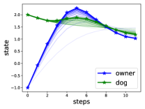
(a) state

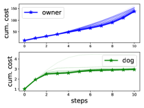
(b) state

Figure 1: Owner-dog dynamic game. In order to keep the dog around $x^{1}=2$, the owner has to overshoot and then come back to $x^{0}=1$. The dog learns to get closer to the owner over iterations, which is what we would expect given how the problem is formulated. As can be seen in Fig. 1(b), the cumulative costs for both players reduces over iterations.

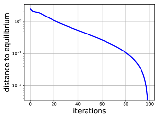
Figure 2: This shows the 2-norm distance between inputs $\bar{u}$ and the final equilibrium $u^{\star}$ over iterations. As can be seen that the error reduces sub-linearly on a log scaled plot, which is evidence that the algorithm converges quadratically.

We consider a simple 1-D owner-dog problem, with horizon $T=11$ and initial state $x_{:,0}=[-1,2]$ where the dynamics of both the owner and the dog are given respectively by

$$x^{0}_{k+1}=x^{0}_{k}+\tanh u^{0}_{k}$$ (30a)

$$x^{1}_{k+1}=x^{1}_{k}+\tanh u^{1}_{k}$$ (30b)

The owner cares about going to $x^{0}=1$ and that the dog can stay at $x^{1}=2$. The dog, however, only tries to catch up with the owner. Each player also concerns itself with the energy consumption, therefore has a cost term related to the magnitude of its input. Their cost functions are formulated as

$$c_{0,k}(x,u)=10\ \text{sigmoid}((x^{0}_{k}-1)^{2})+40(x^{1}_{k}-2)^{2}+(u^{0}_{k})^{2}$$ (31a)

$$c_{1,k}(x,u)=\tanh^{2}(x^{0}_{k}-x^{1}_{k})+(u^{1}_{k})^{2}$$ (31b)

Nonlinear functions are added to the dynamics and costs to create a nonlinear game rather than for explicit physical meaning. We initialize a trajectory with zero input and initial state, i.e. $\bar{u}=[0.,0.,\ldots,0.]$ and $\bar{x}=[-1,2,-1,2,\ldots,-1,2]$. We used an identity regularization matrix with a magnitude of 400.

Fig. 1 shows the solution via DDP to this problem over iterations, where the more transparent the trajectories, the earlier in the iterations they are. The starred trajectory is the final equilibrium solution. We simulated 100 iterations after the initial trajectory and picked 10 uniformly spaced ones to show in the figures.

VI Conclusion

In this paper we have shown how differential dynamic programming extends to dynamic games. The key steps were involved finding explicit forms for both DDP and Newton iterations that enable clean comparison of their solutions. We demonstrated the performance of the algorithm on a simple nonlinear dynamic game.

Many extensions are possible. We will examine larger examples and work on numerical scaling. Also of interest are stochastic dynamic games and problems in which agents have differing, imperfect information sets. Additionally, handling scenarios in which agents have imperfect model information will of great practical importance.

Appendix A Proofs of Lemmas

We first derive a few useful results which we’ll use later in this chapter.

First, we bound the spectral radius of $F_{k}^{-1}$ from above

$$\rho(F_{k}^{-1})\leq\hat{F}$$ (32)

where $\hat{F}$ is a constant. Consider inverting $\nabla_{u}\mathcal{J}(u)$ in Newton’s method by successively eliminating $\delta u_{:,k}$ for $k=T,T-1,\ldots,0$. The $F_{k}$ matrices are exactly the matrices which would be inverted when eliminating $\delta u_{:,k}$. Since $\nabla_{u}\mathcal{J}(u)$ is Lipschitz continuous, its eigenvalues are bounded away from zero in a neighborhood of $u^{\star}$. It follows that the eigenvalues of $F_{K}$ must also be bounded away from zero and $F_{k}^{-1}$ is bounded above.

Secondly, we assert that

$$\Omega_{n,k}=\frac{\partial}{\partial x_{k}}\Big{|}_{\bar{x},\bar{u}}\sum_{i=k}^{T}c_{n,i}(x_{i},u_{:,i})$$ (33)

which means $\Omega_{n,k}$ captures the first-order effect of $x_{k}$ on the sum of all later costs for each player. $\Omega_{n,k}$ is constructed according to (24a). Equation (33) is true for $k=T$ by construction. We proof by induction and assume that (33) holds for $k+1$, i.e. $\Omega_{n,k+1}=\frac{\partial}{\partial x_{k+1}}\Big{|}_{\bar{x},\bar{u}}\sum_{i={k+1}}^{T}c_{n,i}(x_{i},u_{:,i})$, then

$$\Omega_{n,k}=M_{n,k}+\Omega_{n,k+1}A_{k}$$ (34a)

$$=\frac{\partial c_{n,k}(x_{k},u_{:,k})}{x_{k}}\Big{|}_{\bar{x},\bar{u}}+\left(\frac{\partial}{\partial x_{k+1}}\sum_{i=k+1}^{T}c_{n,i}(x_{i},u_{:,i})\right)\frac{\partial x_{k+1}}{\partial x_{k}}\Big{|}_{\bar{x},\bar{u}}$$ (34b)

$$=\frac{\partial c_{n,k}(x_{k},u_{:,k})}{x_{k}}\Big{|}_{\bar{x},\bar{u}}+\left(\frac{\partial}{\partial x_{k}}\Big{|}_{\bar{x},\bar{u}}\sum_{i=k+1}^{T}c_{n,i}(x_{i},u_{:,i})\right)$$ (34c)

$$=\frac{\partial}{\partial x_{k}}\Big{|}_{\bar{x},\bar{u}}\sum_{i=k}^{T}c_{n,i}(x_{i},u_{:,i})$$ (34d)

Therefore, (33) holds for $k$. And by induction, all $k=0,1,\ldots,T$. ∎

The third useful result is that

$$M^{1u}_{n,k}+\Omega_{n,k+1}B_{k}=\frac{\partial J_{n}(u)}{\partial u_{:,k}}\Big{|}_{\bar{u}}=O(\epsilon)$$ (35)

$\frac{\partial J_{n}(u)}{\partial u_{:,k}}\Big{|}_{\bar{u}}=O(\epsilon)$ is true because $J_{n}(u)$ is twice differentiable hence Lipschitz, i.e.

$$\Big{|}\Big{|}\frac{J_{n}(u)}{\partial u_{:,k}}\Big{|}_{\bar{u}}-\frac{J_{n}(u)}{\partial u_{:,k}}\Big{|}_{u^{\star}}\Big{|}\Big{|}^{2}\leq\text{constant}\cdot\|\bar{u}-u^{\star}\|^{2}=O(\epsilon)$$ (36)

The first equality holds because

$$\frac{\partial J(u)}{\partial u_{:,k}}\Big{|}_{\bar{u}}= \frac{\partial}{\partial u_{:,k}}\Big{|}_{\bar{x},\bar{u}}\sum_{i=0}^{T}c_{n,i}(x_{i},u_{:,i})=\frac{\partial}{\partial u_{:,k}}\Big{|}_{\bar{x},\bar{u}}\sum_{i=k}^{T}c_{n,i}(x_{i},u_{:,i})$$ (37a)

$$= \frac{\partial}{\partial u_{:,k}}\Big{|}_{\bar{x},\bar{u}}c_{n,k}(x_{k},u_{:,k})+\frac{\partial}{\partial u_{:,k}}\Big{|}_{\bar{x},\bar{u}}\sum_{i=k+1}^{T}c_{n,i}(x_{i},u_{:,i})$$ (37b)

$$= M_{n,k}^{1u}+\frac{\partial}{\partial x_{k+1}}\Big{|}_{\bar{x},\bar{u}}\sum_{i=k+1}^{T}c_{n,i}(x_{i},u_{:,i})\frac{\partial x_{k+1}}{\partial u_{:,k}}\Big{|}_{\bar{x},\bar{u}}$$ (37c)

$$= M^{1u}_{n,k}+\Omega_{n,k+1}B_{k}$$ (37d)

∎

These results are used implicitly in the later proofs of lemmas.

A-A Proof of Lemma 4

First, we prove that the dynamics constraints (20d) and (20e) are inductive definitions of the following approximation terms:

$$\delta x_{k}=\sum_{i=0}^{T}\frac{\partial x_{k}}{\partial u_{:,i}}\Big{|}_{\bar{x},\bar{u}}\delta u_{:,i}$$ (38a)

$$\Delta x_{k}^{l}=\sum_{i=0}^{T}\sum_{j=0}^{T}\delta u_{:,i}^{\top}{\frac{\partial^{2}x_{k}^{l}}{\partial u_{:,i}\partial u_{:,j}}}\Big{|}_{\bar{x},\bar{u}}\delta u_{:,j},\ l=1,2,\ldots,n_{x}$$ (38b)

Note that $x_{0}$ is fixed so that (38) holds at $k=0$. Now we handle each of the terms inductively.

For $\delta x_{k+1}$, we have

$$\delta x_{k+1}=\sum_{i=0}^{T}\frac{\partial x_{k+1}}{\partial u_{:,i}}\Big{|}_{\bar{x},\bar{u}}\delta u_{:,i}$$

$$=\sum_{i=0}^{T}\frac{\partial f_{k}(x_{k},u_{:,k})}{\partial u_{:,i}}\Big{|}_{\bar{x},\bar{u}}\delta u_{:,i}$$

$$=\frac{\partial f_{k}(x_{k},u_{:,k})}{\partial x_{k}}\Big{|}_{\bar{x},\bar{u}}\sum_{i=0}^{T}\frac{\partial x_{k}}{\partial u_{:,k}}\delta u_{:,i}+\frac{\partial f_{k}(x_{k},u_{:,k})}{\partial u_{:,k}}\Big{|}_{\bar{x},\bar{u}}\delta u_{:,k}$$

$$=A_{k}\delta x_{k}+B_{k}\delta u_{:,k}$$ (39)

We used the fact that $\frac{\partial f(x_{k},u_{:,k})}{\partial u_{:,i}}$ is zero unless $i=k$.

For $\Delta x_{k+1}$, row $l$ is given by:

$$\Delta x_{k+1}^{l}=\sum_{i=0}^{T}\sum_{j=0}^{T}\delta u_{:,i}^{\top}{\frac{\partial^{2}f^{l}_{k}(x_{k},u_{:,k})}{\partial u_{:,i}\partial u_{:,j}}}\Big{|}_{\bar{u}}\delta u_{:,j}$$ (40a)

$$=\sum_{i=0}^{T}\sum_{j=0}^{T}\delta u_{:,i}^{\top}\left(\frac{\partial^{2}f^{l}_{k}}{\partial u_{:,i}\partial u_{:,j}}+(\frac{\partial x_{k}}{\partial u_{:,i}})^{\top}\frac{\partial^{2}f^{l}_{k}}{\partial x_{k}^{2}}\frac{\partial x_{k}}{\partial u_{:,j}}\right)\Big{|}_{\bar{u}}\delta u_{:,j}$$

$$+\sum_{i=0}^{T}\sum_{j=0}^{T}\delta u_{:,i}^{\top}\left((\frac{x_{k}}{\partial u_{:,i}})^{\top}\frac{\partial^{2}f^{l}_{k}}{\partial x_{k}\partial u_{:,j}}+\frac{\partial^{2}f^{l}_{k}}{\partial u_{:,i}\partial x_{k}}\frac{x_{k}}{\partial u_{:,j}}\right)\Big{|}_{\bar{u}}\delta u_{:,j}$$

$$+\sum_{i=0}^{T}\sum_{j=0}^{T}\delta u_{:,i}^{\top}\left(\sum_{p=1}^{n_{x}}\frac{\partial f^{l}_{k}}{\partial x^{p}_{k}}\frac{\partial^{2}x^{p}_{k}}{\partial u_{:,i}\partial u_{:,j}}\right)\Big{|}_{\bar{u}}\delta u_{:,j}$$ (40b)

$$=\delta u_{:,k}^{\top}\frac{\partial^{2}f^{l}_{k}}{\partial u_{:,k}^{2}}\delta u_{:,k}+\delta x_{k}^{\top}\frac{\partial^{2}f^{l}_{k}}{\partial x_{k}^{2}}\delta x_{k}+\delta x_{k}^{\top}\frac{\partial^{2}f^{l}_{k}}{\partial x_{k}\partial u_{:,k}}\delta u_{:,k}$$

$$+\delta u_{:,k}^{\top}\frac{\partial^{2}f^{l}_{k}}{\partial u_{:,k}\partial x_{k}}\delta x_{k}+\sum_{p=1}^{n_{x}}\frac{\partial f^{l}_{k}}{\partial x^{p}_{k}}\sum_{i=0}^{T}\sum_{j=0}^{T}\delta u_{:,i}^{\top}{\frac{\partial^{2}x^{p}_{k}}{\partial u_{:,i}\partial u_{:,j}}}\delta u_{:,j}$$ (40c)

$$=\begin{bmatrix}\delta x_{k}\\ \delta u_{:,k}\end{bmatrix}^{\top}G^{l}_{k}\begin{bmatrix}\delta x_{k}\\ \delta u_{:,k}\end{bmatrix}+\sum_{p=1}^{n_{x}}A^{lp}_{k}\Delta x_{k}^{p}$$ (40d)

To get to each terms in (40c), we used the fact that

$$\frac{\partial^{2}f^{l}_{k}}{\partial u_{:,i}\partial u_{:,j}}=0,\ \text{for}\ i\neq k\ \text{or}\ j\neq k$$ (41a)

$$\delta x_{k}=\sum_{i=0}^{T}\frac{\partial x_{k}}{\partial u_{:,i}}\delta u_{:,i}=\sum_{i=0}^{k-1}\frac{\partial x_{k}}{\partial u_{:,i}}\delta u_{:,i}$$ (41b)

To get to (40d), we used the fact

$$\frac{\partial f^{l}_{k}}{\partial x^{p}_{k}}=A^{lp}_{k}$$ (42a)

$$\sum_{i=0}^{T}\sum_{j=0}^{T}\delta u_{:,i}^{\top}{\frac{\partial^{2}x^{p}_{k}}{\partial u_{:,i}\partial u_{:,j}}}\Big{|}_{\bar{u}}\delta u_{:,j}=\Delta x_{k}^{p}$$ (42b)

$$\begin{bmatrix}\frac{\partial^{2}f^{l}_{k}}{\partial x_{k}^{2}}&\frac{\partial^{2}f^{l}_{k}}{\partial x_{k}\partial u_{:,k}}\\ \frac{\partial^{2}f^{l}_{k}}{\partial x_{k}\partial u_{:,k}}&\frac{\partial^{2}f^{l}_{k}}{\partial u_{:,k}^{2}}\end{bmatrix}\Bigg{|}_{\bar{x},\bar{u}}=G^{l}_{k}$$ (42c)

Both $l$ and $p$ are used to pick out the corresponding element for a vector or matrix. $A^{lp}_{k}$ means the $l$th row and $p$th column of matrix $A_{k}$. Equation (40d) actually describes each element in (38b), so we’ve proven that both are true.

Next we prove (20a) is the quadratic approximation of $J_{n}(u)$, i.e.

$$\text{quad}(J_{n}(u))_{\bar{u}}=J_{n}(\bar{u})+\frac{\partial J_{n}^{T}(\bar{u})}{\partial u}+\frac{1}{2}\delta u^{T}\frac{\partial^{2}J_{n}(\bar{u})}{\partial u^{2}}\delta u$$

$$=\frac{1}{2}\sum_{k=0}^{T}\left(\begin{bmatrix}1\\ \delta x_{k}\\ \delta u_{:,k}\end{bmatrix}^{T}M_{n,k}\begin{bmatrix}1\\ \delta x_{k}\\ \delta u_{:,k}\end{bmatrix}+M^{1k}_{n,k}\Delta x_{k}\right)$$ (43)

We’ll need the explicit expressions for the associated derivatives.

$$\frac{\partial J_{n}(u)}{\partial u_{:,i}}=\sum_{k=0}^{T}\left(\frac{\partial c_{n,k}(x_{k},u_{:,k})}{\partial u_{:,i}}+\frac{\partial c_{n,k}(x_{k},u_{:,k})}{\partial x_{k}}\frac{\partial x_{k}}{\partial u_{:,i}}\right)$$ (44a)

$$\frac{\partial^{2}J_{n}(u)}{\partial u_{:,i}\partial u_{:,j}}$$

$$=\sum_{k=0}^{T}\left(\frac{\partial^{2}c_{n,k}(x_{k},u_{:,k})}{\partial u_{:,i}\partial u_{:,j}}+\frac{\partial x_{k}}{\partial u_{:,i}}^{\top}\frac{\partial^{2}c_{n,k}(x_{k},u_{:,k})}{\partial x_{k}^{2}}\frac{\partial x_{k}}{\partial u_{:,j}}\right)$$

$$+\sum_{k=0}^{T}\left(\frac{\partial x_{k}}{\partial u_{:,i}}^{\top}\frac{\partial^{2}c_{n,k}(x_{k},u_{:,k})}{\partial x_{k}\partial u_{:,j}}+\frac{\partial^{2}c_{n,k}(x_{k},u_{:,k})}{\partial u_{:,i}\partial x_{k}}\frac{\partial x_{k}}{\partial u_{:,j}}\right)$$

$$+\sum_{k=0}^{T}\sum_{l=1}^{n_{x}}\frac{\partial c_{n,k}(x_{k},u_{:,k})}{\partial x_{k}^{l}}\frac{\partial^{2}x_{k}^{l}}{\partial u_{:,i}\partial u_{:,i}}$$ (44b)

We break down each term in (A-A). First the second order term.

$$\delta u^{T}\frac{\partial^{2}J_{n}(\bar{u})}{\partial u^{2}}\delta u=\sum_{i,j=0}^{T}\delta u_{:,i}^{T}\frac{\partial^{2}J_{n}(u)}{\partial u_{:,i}\partial u_{:,j}}\bigg{|}_{\bar{u}}\delta u_{:,j}$$ (45a)

$$=\sum_{i,j,k=0}^{T}\delta u_{:,i}^{T}\left(\frac{\partial^{2}c_{n,k}(x_{k},u_{:,k})}{\partial u_{:,i}\partial u_{:,j}}\bigg{|}_{\bar{u}}\right)\delta u_{:,j}$$

$$+\sum_{i,j,k=0}^{T}\delta u_{:,i}^{T}\left(\frac{\partial x_{k}}{\partial u_{:,i}}^{\top}\frac{\partial^{2}c_{n,k}(x_{k},u_{:,k})}{\partial x_{k}^{2}}\bigg{|}_{\bar{u}}\frac{\partial x_{k}}{\partial u_{:,j}}\right)\delta u_{:,j}$$

$$+\sum_{i,j,k=0}^{T}\delta u_{:,i}^{T}\left(\frac{\partial x_{k}}{\partial u_{:,i}}^{\top}\frac{\partial^{2}c_{n,k}(x_{k},u_{:,k})}{\partial x_{k}\partial u_{:,j}}\bigg{|}_{\bar{u}}\right)\delta u_{:,j}$$

$$+\sum_{i,j,k=0}^{T}\delta u_{:,i}^{T}\left(\frac{\partial^{2}c_{n,k}(x_{k},u_{:,k})}{\partial u_{:,i}\partial x_{k}}\bigg{|}_{\bar{u}}\frac{\partial x_{k}}{\partial u_{:,j}}\right)\delta u_{:,j}$$

$$+\sum_{k=0}^{T}\sum_{p=1}^{n}\frac{\partial c_{n,k}(x_{k},u_{:,k})}{\partial x_{k}^{p}}\bigg{|}_{\bar{u}}\sum_{i,j=0}^{T}\delta u_{:,i}^{T}\frac{\partial^{2}x_{k}^{p}}{\partial u_{:,i}\partial u_{:,i}}\delta u_{:,j}$$ (45b)

$$= \sum_{k=0}^{T}\left(\delta u_{:,k}^{\top}\frac{\partial^{2}c_{n,k}}{\partial u_{:,k}^{2}}\bigg{|}_{\bar{u}}\delta u_{:,k}+\delta x_{k}^{\top}\frac{\partial^{2}c_{n,k}}{\partial x_{k}^{2}}\bigg{|}_{\bar{u}}\delta x_{k}\right)+$$

$$\sum_{k=0}^{T}\left(\delta x_{k}^{\top}\frac{\partial^{2}c_{n,k}}{\partial x_{k}\partial u_{:,k}}|_{\bar{u}}\delta u_{:,k}+\delta u_{:,k}^{\top}\frac{\partial^{2}c_{n,k}}{\partial u_{:,k}\partial x_{k}}\bigg{|}_{\bar{u}}\delta x_{k}\right)+$$

$$\sum_{k=0}^{T}\sum_{p=1}^{n}\frac{\partial c_{n,k}(x_{k},u_{:,k})}{\partial x_{k}^{p}}\Delta x_{k}^{p}$$ (45c)

$$= \sum_{k=0}^{T}\left(\begin{bmatrix}\delta x_{k}\\ \delta u_{:,k}\end{bmatrix}^{T}\begin{bmatrix}\frac{\partial^{2}c_{n,k}}{\partial x_{k}^{2}}&\frac{\partial^{2}c_{n,k}}{\partial x_{k}\partial u_{:,k}}\\ \frac{\partial^{2}c_{n,k}}{\partial u_{:,k}\partial x_{k}}&\frac{\partial^{2}c_{n,k}}{\partial u_{:,k}^{2}}\end{bmatrix}\bigg{|}_{\bar{u}}\begin{bmatrix}\delta x_{k}\\ \delta u_{:,k}\end{bmatrix}\right)$$

$$+\left(\frac{\partial c_{n,k}(x_{k},u_{:,k})}{\partial x_{k}}\Delta x_{k}\right)$$ (45d)

The first term in (45) to (45) holds because $c_{n,k}(x_{k},u_{:,k})$ only depends directly on $u_{:,i}$ and $u_{:,j}$ when $i=j=k$. The others hold because $x_{k}$ only depends on $u_{:,i}$ and $u_{:,j}$ when $i,j<k$. The last term uses the definition of $\Delta x_{k}$ in (38b).

The first order term

$$\frac{\partial J_{n}(\bar{u})}{\partial u}=\sum_{i=0}^{T}\frac{\partial J_{n}(u)}{\partial u_{:,i}}\delta u_{:,i}$$ (46a)

$$=\sum_{i,k=0}^{T}\left(\frac{\partial c_{n,k}(x_{k},u_{:,k})}{\partial u_{:,i}}+\frac{\partial c_{n,k}(x_{k},u_{:,k})}{\partial x_{k}}\frac{\partial x_{k}}{\partial u_{:,i}}\right)\delta u_{:,i}$$ (46b)

$$=\sum_{k=0}^{T}\left(\frac{\partial c_{n,k}(x_{k},u_{:,k})}{\partial u_{:,k}}\delta u_{:,k}+\frac{\partial c_{n,k}(x_{k},u_{:,k})}{\partial x_{k}}\sum_{i=0}^{T}\frac{\partial x_{k}}{\partial u_{:,i}}\right)$$ (46c)

$$=\sum_{k=0}^{T}\left(\frac{\partial c_{n,k}(x_{k},u_{:,k})}{\partial u_{:,k}}\delta u_{:,k}+\frac{\partial c_{n,k}(x_{k},u_{:,k})}{\partial x_{k}}\delta x_{k}\right)$$ (46d)

And constant term

$$J_{n}(\bar{u})=\sum_{k=0}^{T}c_{n,k}(\bar{x}_{k},\bar{u}_{:,k})$$ (47)

From (45), (46), and (47) it follows that (A-A) is true. ∎

A-B Proof of Lemma 6

A more complete version of Lemma 6 is

$$\tilde{D}_{n,k} =D_{n,k}+O(\epsilon)$$ (48a)

$$S^{1x}_{n,k} =\Omega_{n,k}+O(\epsilon)$$ (48b)

$$\tilde{S}^{1x}_{n,k} =\Omega_{n,k}+O(\epsilon)$$ (48c)

$$\tilde{S}^{1x}_{n,k} =S^{1x}_{n,k}+O(\epsilon^{2})$$ (48d)

$$\tilde{S}_{n,k} =S_{n,k}+O(\epsilon)$$ (48e)

$$\begin{bmatrix}\tilde{\Gamma}^{1x}_{n,k}&\tilde{\Gamma}^{1u}_{n,k}\end{bmatrix} =\begin{bmatrix}\Gamma^{1x}_{n,k}&\Gamma^{1u}_{n,k}\end{bmatrix}+O(\epsilon^{2})$$ (48f)

$$\tilde{\Gamma}_{n,k} =\Gamma_{n,k}+O(\epsilon)$$ (48g)

$$\Gamma_{n,k}^{1u} =O(\epsilon)$$ (48h)

$$\tilde{\Gamma}_{n,k}^{1u} =O(\epsilon)$$ (48i)

$$\tilde{F}_{k} =F_{k}+O(\epsilon)$$ (48j)

$$\tilde{P}_{k} =P_{k}+O(\epsilon)$$ (48k)

$$\tilde{H}_{k} =H_{k}+O(\epsilon^{2})$$ (48l)

$$\tilde{H}_{k} =O(\epsilon)$$ (48m)

$$H_{k} =O(\epsilon)$$ (48n)

$$\tilde{s}_{k} =s_{k}+O(\epsilon^{2})$$ (48o)

$$\tilde{s}_{k} =O(\epsilon)$$ (48p)

$$s_{k} =O(\epsilon)$$ (48q)

$$\tilde{K}_{k} =K_{k}+O(\epsilon),$$ (48r)

of which we give a proof by induction for in this section.

For $k=T$, because of the way these variables are constructed, they are identical, i.e.

$$\Gamma_{n,T}= \tilde{\Gamma}_{n,T}$$ (49a)

$$F_{T}= \tilde{F}_{T}$$ (49b)

$$P_{T}= \tilde{P}_{T}$$ (49c)

$$H_{T}= \tilde{H}_{T}$$ (49d)

$$s_{T}= \tilde{s}_{T}$$ (49e)

$$K_{T}= \tilde{K}_{T}$$ (49f)

$$S_{n,T}= \tilde{S}_{n,T}$$ (49g)

So we have (48d)(48e)(48f)(48g)(48j)(48k)(48l)(48o)(48r) hold for $k=T$.

We also know that

$$M_{n,T}^{1u}=\frac{\partial c_{n,T}}{\partial u_{T}}=\frac{\partial J_{n}(u)}{\partial u_{T}}=O(\epsilon)$$ (50)

where the first equality is by construction, the second is true because $u_{T}$ only appears in $J_{n}(u)$ in $c_{n,T}$. By construction, $\Gamma_{n,T}^{1u}=\tilde{\Gamma}_{n,T}^{1u}=M_{n,T}^{1u}=O(\epsilon)$, so (48h)(48i) are true for $k=T$.
Similarly, $H_{T}$ and $\tilde{H}_{T}$ are constructed from $\Gamma_{n,T}^{u1}$ and $\tilde{\Gamma}_{n,T}^{u1}$, so (48m)(48n) are true for $k=T$.

Because $F_{k}^{-1}$ is bounded above, $s_{T}=-F_{T}^{-1}H_{T}=-F_{T}^{-1}O(\epsilon)=O(\epsilon)$. Similarly, $\tilde{s}_{T}=O(\epsilon)$. Equations (48p)(48q) are true for $k=T$.

From (24h) and $\Gamma_{n,T}=M_{n,T}$, we can get

$$S_{n,T}^{1x}= M_{n,T}^{1x}+M_{n,T}^{1u}K_{T}+s_{T}^{\top}(M_{n,T}^{ux}+M_{n,T}^{uu}K_{T})$$ (51a)

$$= \Omega_{n,T}+O(\epsilon)K_{T}+O(\epsilon)(M_{n,T}^{ux}+M_{n,T}^{uu}K_{T})$$ (51b)

$$= \Omega_{n,T}+O(\epsilon)$$ (51c)

because $M_{n,T}$ is bounded. Hence (48b) is true. Further, (48c) is also true.

The time indices for $D_{n,T-1}$ and $\tilde{D}_{n,T-1}$ go to a maximum of $T-1$, so to prove things inductively, we need (48a) to hold for $k=T-1$.The difference between constructions of $D_{n,T-1}$ and $\tilde{D}_{n,T-1}$ is in that the former uses $\Omega_{n,T}$ and the later uses $\tilde{S}_{n,T}^{1x}$. But since we’ve proven $\Omega_{n,T}=\tilde{S}_{n,T}^{1x}+O(\epsilon)$, and $G_{T-1}$ is bounded, we can also conclude $D_{n,T-1}=\tilde{D}_{n,T-1}+O(\epsilon)$. Therefore (48a) is true for $k=T-1$.

So far, we’ve proved that for the last step, either $k=T$ or $k=T-1$, (48) is true. Assuming except for (48a), (48) is true for $k+1$ and (48a) is true for $k$. If we can prove all equations hold one step back, our proof by induction would be done.

Assume (48a) holds for $k$ and other equations in (48) hold for $k+1$. Readers be aware that we’ll use these assumptions implicitly in the derivations following.

From (24) we can get

$$\Gamma_{n,k}^{1u}= M_{k,T}^{1u}+S_{n,k+1}^{1x}B_{k}$$ (52a)

$$= M_{k,T}^{1u}+\Omega_{n,k+1}B_{k}+O(\epsilon)B_{k}$$ (52b)

$$= O(\epsilon)$$ (52c)

Here we used (35). Similarly, we can prove $\tilde{\Gamma}_{n,k}^{1u}=O(\epsilon)$. So (48h) and (48i) hold for $k$.

From (24) and (15b) we can compute the difference between $\tilde{\Gamma}_{n,k}$ and $\Gamma_{n,k}$ as

$$\ \tilde{\Gamma}_{n,k}-\Gamma_{n,k}$$

$$= \begin{bmatrix}\tilde{S}_{n,k+1}^{11}-S_{n,k+1}^{11}&\mathbf{0}&\mathbf{0}\\ A_{k}^{\top}(\tilde{S}_{n,k+1}^{x1}-S_{n,k+1}^{x1})&\mathbf{0}&\mathbf{0}\\ B_{k}^{\top}(\tilde{S}_{n,k+1}^{x1}-S_{n,k+1}^{x1})&\mathbf{0}&\mathbf{0}\end{bmatrix}$$

$$+\begin{bmatrix}\mathbf{0}&(\tilde{S}_{n,k+1}^{1x}-S_{n,k+1}^{1x})A_{k}&\mathbf{0}\\ \mathbf{0}&A_{k}^{\top}(\tilde{S}_{n,k+1}^{xx}-S_{n,k+1}^{xx})A_{k}+(\tilde{D}_{k}^{xx}-D_{k}^{xx})&\mathbf{0}\\ \mathbf{0}&B_{k}^{\top}(\tilde{S}_{n,k+1}^{xx}-S_{n,k+1}^{xx})A_{k}+(\tilde{D}_{k}^{ux}-D_{k}^{ux})&\mathbf{0}\end{bmatrix}$$

$$+\begin{bmatrix}\mathbf{0}&\mathbf{0}&(\tilde{S}_{n,k+1}^{1x}-S_{n,k+1}^{1x})B_{k}\\ \mathbf{0}&\mathbf{0}&A_{k}^{\top}(\tilde{S}_{n,k+1}^{xx}-S_{n,k+1}^{xx})B_{k}+(\tilde{D}_{k}^{xu}-D_{k}^{xu})\\ \mathbf{0}&\mathbf{0}&B_{k}^{\top}(\tilde{S}_{n,k+1}^{xx}-S_{n,k+1}^{xx})B_{k}+(\tilde{D}_{k}^{uu}-D_{k}^{uu})\end{bmatrix}$$ (53a)

$$= \begin{bmatrix}O(\epsilon)&A_{k}O(\epsilon^{2})&B_{k}O(\epsilon^{2})\\ A_{k}^{\top}O(\epsilon^{2})&A_{k}^{\top}O(\epsilon)A_{k}+O(\epsilon)&A_{k}^{\top}O(\epsilon)B_{k}+O(\epsilon)\\ B_{k}^{\top}O(\epsilon^{2})&B_{k}^{\top}O(\epsilon)A_{k}+O(\epsilon)&B_{k}^{\top}O(\epsilon)B_{k}+O(\epsilon)\end{bmatrix}$$ (53b)

$$= \begin{bmatrix}O(\epsilon)&O(\epsilon^{2})&O(\epsilon^{2})\\ O(\epsilon^{2})&O(\epsilon)&O(\epsilon)\\ O(\epsilon^{2})&O(\epsilon)&O(\epsilon)\end{bmatrix}$$ (53c)

from which we can see that (48f) and (48g) are true. Once we proved the closeness between $\tilde{\Gamma}_{n,k}$ and $\Gamma_{n,k}$ and the specific terms are $O(\epsilon)$, i.e. (48f) to (48i), because of they way they are constructed from $\tilde{\Gamma}_{n,k}$ and $\Gamma_{n,k}$, we are safe to say

$$\tilde{F}_{k} =F_{k}+O(\epsilon)$$ (54a)

$$\tilde{P}_{k} =P_{k}+O(\epsilon)$$ (54b)

$$\tilde{H}_{k} =H_{k}+O(\epsilon^{2})$$ (54c)

$$\tilde{H}_{k} =O(\epsilon)$$ (54d)

$$H_{k} =O(\epsilon)$$ (54e)

Therefore, (48j), (48k), (48l), (48m) and (48n) are true for $k$.

Now that we have the results with $F_{k}$, $\tilde{F}_{k}$, $H_{k}$, $\tilde{H}_{k}$, $P_{k}$ and $\tilde{P}_{k}$, we can move to what are immediately following, i.e. $s_{k}$, $\tilde{s}_{k}$, $K_{k}$ and $\tilde{K}_{k}$.

$$s_{k}= -F_{k}^{-1}H_{k}=-F_{k}^{-1}O(\epsilon)=O(\epsilon)$$ (55)

which is true because $F_{k}^{-1}$ is bounded above. Similarly, we have $\tilde{s}_{k}=O(\epsilon)$. Equations (48p) and (48q) are true.

$$\tilde{s}_{k} =-\tilde{F}_{k}^{-1}\tilde{H}_{k}=-(F_{k}+O(\epsilon))^{-1}(H_{k}+O(\epsilon^{2}))$$ (56a)

$$=-(F_{k}^{-1}+O(\epsilon))(H_{k}+O(\epsilon^{2}))$$ (56b)

$$=-F_{k}^{-1}H_{k}+F_{k}^{-1}O(\epsilon^{2})+H_{k}O(\epsilon)+O(\epsilon^{2})$$ (56c)

$$=s_{k}+O(\epsilon^{2})$$ (56d)

$$\tilde{K}_{k} =-\tilde{F}_{k}^{-1}\tilde{P}_{k}=-(F_{k}+O(\epsilon))^{-1}(P_{k}+O(\epsilon))$$ (56e)

$$=-(F_{k}^{-1}+O(\epsilon))(P_{k}+O(\epsilon))$$ (56f)

$$=-F_{k}^{-1}P_{k}+(F_{k}^{-1}+P_{k})O(\epsilon)+O(\epsilon^{2})$$ (56g)

$$=K_{k}+O(\epsilon)$$ (56h)

Equations (48o) and (48r) are true for $k$.

Now we are equipped to get closeness/small results for $S_{n,k}$ and $\tilde{S}_{n,k}$.

$$\ \tilde{S}_{n,k}-S_{n,k}$$

$$= \begin{bmatrix}1&0&0\\ 0&I&\tilde{K}_{k}^{\top}\end{bmatrix}\tilde{\Gamma}_{n,k}\begin{bmatrix}1&0\\ 0&I\\ 0&\tilde{K}_{k}\end{bmatrix}-\begin{bmatrix}1&0&0\\ 0&I&K_{k}^{\top}\end{bmatrix}\Gamma_{n,k}\begin{bmatrix}1&0\\ 0&I\\ 0&K_{k}\end{bmatrix}$$

$$+\begin{bmatrix}\tilde{s}_{k}^{\top}\tilde{\Gamma}_{n,k}^{uu}\tilde{s}_{k}+2\tilde{s}_{k}^{\top}\tilde{\Gamma}_{n,k}^{u1}-s_{k}^{\top}\Gamma_{n,k}^{uu}s_{k}-2s_{k}^{\top}\Gamma_{n,k}^{u1}&\mathbf{0}\\ (\tilde{\Gamma}_{n,k}^{xu}+\tilde{\Gamma}_{n,k}^{uu}\tilde{K}_{k})\tilde{s}_{k}-(\Gamma_{n,k}^{ux}+\Gamma_{n,k}^{uu}K_{k})^{\top}s_{k}&\mathbf{0}\end{bmatrix}$$

$$+\begin{bmatrix}\mathbf{0}&\tilde{s}_{k}^{\top}(\tilde{\Gamma}_{n,k}^{ux}+\tilde{\Gamma}_{n,k}^{uu}\tilde{K}_{k})-s_{k}^{\top}(\Gamma_{n,k}^{ux}+\Gamma_{n,k}^{uu}K_{k})\\ \mathbf{0}&\mathbf{0}\end{bmatrix}$$ (57a)

$$= \begin{bmatrix}\tilde{\Gamma}_{n,k}^{11}&\tilde{\Gamma}_{n,k}^{1x}+\tilde{\Gamma}_{n,k}^{1u}\tilde{K}\\ \tilde{\Gamma}_{n,k}^{x1}+\tilde{K}^{\top}\tilde{\Gamma}_{n,k}^{u1}&\tilde{\Gamma}_{n,k}^{xx}+2\tilde{\Gamma}_{n,k}^{xu}\tilde{K}+\tilde{K}^{\top}\tilde{\Gamma}_{n,k}^{uu}\tilde{K}\end{bmatrix}$$

$$-\begin{bmatrix}\Gamma_{n,k}^{11}&\Gamma_{n,k}^{1x}+\Gamma_{n,k}^{1u}K\\ \Gamma_{n,k}^{x1}+K^{\top}\Gamma_{n,k}^{u1}&\Gamma_{n,k}^{xx}+2\Gamma_{n,k}^{xu}K+K^{\top}\Gamma_{n,k}^{uu}K\end{bmatrix}$$

$$+\begin{bmatrix}O(\epsilon)&O(\epsilon^{2})\\ O(\epsilon)&0\end{bmatrix}$$ (57b)

$$= \begin{bmatrix}O(\epsilon)&O(\epsilon^{2})\\ O(\epsilon^{2})&O(\epsilon)\end{bmatrix}$$ (57c)

So that (48d) and (48e) are true for $k$.

$$S_{n,k}^{1x}=M_{n,k}^{1x}+S_{n,k+1}^{1x}A_{k}+\Gamma_{n,k}^{1u}K_{k}+s_{k}^{\top}(\Gamma_{n,k}^{ux}+\Gamma_{n,k}^{uu}K_{k})$$ (58a)

$$=M_{n,k}^{1x}+\Omega_{n,k+1}A_{k}+A_{k}O(\epsilon)$$

$$\quad+K_{k}O(\epsilon)+(\Gamma_{n,k}^{ux}+\Gamma_{n,k}^{uu}K_{k})O(\epsilon)$$ (58b)

$$=\Omega_{n,k}+O(\epsilon)$$ (58c)

Therefore, (48b) holds and then naturally (48c) holds.

We continue to prove that $\tilde{D}_{n,k-1}$ and $D_{n,k-1}$ are close, which is true because

$$\tilde{D}_{n,k-1}= \sum_{l=1}^{n_{x}}\tilde{S}_{n,k}^{1x^{l}}G_{k}^{l}$$ (59a)

$$= \sum_{l=1}^{n_{x}}(\Omega_{n,k}^{l}+O(\epsilon))G_{k}^{l}$$ (59b)

$$= \sum_{l=1}^{n_{x}}\Omega_{n,k}^{l}G_{k}^{l}+O(\epsilon)$$ (59c)

$$= D_{n,k-1}+O(\epsilon)$$ (59d)

So (48a) is true. ∎

A-C Proof of Lemma 7

A more complete version of Lemma 7 is

$$\delta x_{k+1}^{D}= A_{k}\delta x_{k}^{D}+B_{k}\delta u_{k}^{D}+O(\epsilon^{2})$$ (60a)

$$\delta x_{k+1}^{N}= A_{k}\delta x_{k}^{N}+B_{k}\delta u_{k}^{N}+O(\epsilon^{2})$$ (60b)

$$\delta u_{k}^{N}=O(\epsilon)$$ (60c)

$$\delta u_{k}^{D}=O(\epsilon)$$ (60d)

$$\delta x_{k}^{N}=O(\epsilon)$$ (60e)

$$\delta x_{k}^{D}=O(\epsilon)$$ (60f)

$$\delta u_{k}^{N}-\delta u_{k}^{D}= O(\epsilon^{2})$$ (60g)

$$\delta x_{k}^{N}-\delta x_{k}^{D}= O(\epsilon^{2})$$ (60h)

$$\delta u^{N}-\delta u^{D}= O(\epsilon^{2})$$ (60i)

$$\|\bar{u}+\delta u^{N}-u^{\star}\|= O(\epsilon^{2}).$$ (60j)

$$\|\bar{u}+\delta u^{D}-u^{\star}\|= O(\epsilon^{2}).$$ (60k)

Equation (60a) comes directly from the Taylor series expansion of (2) and (60b) from (20d).

We prove (60c) to (60h) by induction. For $k=0$, $\delta x_{0}^{N}=\delta x_{0}^{D}=0$ and $\delta u_{0}^{N}=s_{0},\ \delta x_{0}^{D}=\tilde{s}_{0}$. We know from the proof of lemma 6 that $s_{0}=\tilde{s}_{0}+O(\epsilon^{2})$, $s_{0}=O(\epsilon)$ and $\tilde{s}_{0}=O(\epsilon)$, so (60c) to (60h) hold for $k=0$. Assume (60c) to (60h) hold for $k$, then

$$\delta u^{N}_{k+1} =K_{k+1}\delta x^{N}_{k}+s_{k+1}=O(\epsilon)$$ (61a)

$$\delta u^{D}_{k+1} =\tilde{K}_{k+1}\delta x^{N}_{k}+\tilde{s}_{k+1}=O(\epsilon)$$ (61b)

$$\delta x^{N}_{k+1}= A_{k}\delta x^{N}_{k}+B_{k}\delta u^{N}_{k}+O(\epsilon^{2})=O(\epsilon)$$ (61c)

$$\delta x^{D}_{k+1}= A_{k}\delta x^{D}_{k}+B_{k}\delta u^{D}_{k}+O(\epsilon^{2})=O(\epsilon)$$ (61d)

$$\delta u^{N}_{k+1}-\delta u^{D}_{k+1}= K_{k}\delta x^{N}_{k}-\tilde{K}_{k}\delta x^{D}_{k}+s_{k}-\tilde{s}_{k}$$ (61e)

$$= K_{k}\delta x^{N}_{k}-(K_{k}+O(\epsilon))(\delta x^{N}_{k}+O(\epsilon^{2}))$$

$$+O(\epsilon^{2})$$ (61f)

$$= O(\epsilon)\delta x^{N}_{k}+O(\epsilon^{2})$$ (61g)

$$= O(\epsilon^{2})$$ (61h)

$$\delta x^{N}_{k+1}-\delta x^{D}_{k+1}= A_{k}(\delta x^{N}_{k}-\delta x^{D}_{k})+B_{k}(\delta u^{N}_{k}-\delta u^{D}_{k})+O(\epsilon^{2})$$

$$= O(\epsilon^{2})$$ (61i)

So (60c) to (60h) hold for $k+1$ and the proof by induction is done. Equation (60i) comes directly as a result. Equation (60j) is classic convergence analysis for Newton’s method [24]. Equation (60k) follows directly from (60i) and (60j). ∎

A-D Proof of Lemma 1

As discussed in the proof of Lemma 2, a necessary condition for the solution of (10c) is given by (16). Thus, a sufficient condition for a unique solution is that $\tilde{F}_{k}$ be invertible. At the beginning of the appendix, whe showed that $F_{k}^{-1}$ exists near $u^{\star}$ and that its spectral radius is bounded.

Now we show that $\tilde{F}_{k}$ exists and $\rho(\tilde{F}_{k}^{-1})$ is bounded. Lemma 6 implies that $\tilde{F}_{k}=F_{k}+O(\epsilon)$. It follows that

$$\tilde{F}_{k}^{-1}=(F_{k}+O(\epsilon))^{-1}=F_{k}^{-1}-F_{k}^{-1}O(\epsilon)F_{k}^{-1}=F_{k}^{-1}+O(\epsilon).$$

It follows that $\tilde{F}_{k}^{-1}$ exists and is bounded in a neighborhood of $u^{\star}$. ∎

References

- [1] I. Rusnak, “The lady, the bandits, and the bodyguards–a two team dynamic game,” in Proceedings of the 16th world IFAC congress, 2005, pp. 934–939.
- [2] O. Prokopov and T. Shima, “Linear quadratic optimal cooperative strategies for active aircraft protection,” Journal of Guidance, Control, and Dynamics, vol. 36, no. 3, pp. 753–764, 2013.
- [3] E. Garcia, D. W. Casbeer, K. Pham, and M. Pachter, “Cooperative aircraft defense from an attacking missile,” in Decision and Control (CDC), 2014 IEEE 53rd Annual Conference on. IEEE, 2014, pp. 2926–2931.
- [4] F. El Ouardighi, S. Jørgensen, and F. Pasin, “A dynamic game with monopolist manufacturer and price-competing duopolist retailers,” OR spectrum, vol. 35, no. 4, pp. 1059–1084, 2013.
- [5] Q. Zhu, Z. Han, and T. Başar, “A differential game approach to distributed demand side management in smart grid,” in Communications (ICC), 2012 IEEE International Conference on. IEEE, 2012, pp. 3345–3350.
- [6] D. H. Jacobson, “New second-order and first-order algorithms for determining optimal control: A differential dynamic programming approach,” Journal of Optimization Theory and Applications, vol. 2, no. 6, pp. 411–440, 1968.
- [7] W. Sun, E. A. Theodorou, and P. Tsiotras, “Game theoretic continuous time differential dynamic programming,” in American Control Conference (ACC), 2015. IEEE, 2015, pp. 5593–5598.
- [8] ——, “Stochastic game theoretic trajectory optimization in continuous time,” in Decision and Control (CDC), 2016 IEEE 55th Conference on. IEEE, 2016, pp. 6167–6172.
- [9] T. Basar and G. J. Olsder, Dynamic noncooperative game theory. Siam, 1999, vol. 23.
- [10] D. Murray and S. Yakowitz, “Differential dynamic programming and newton’s method for discrete optimal control problems,” Journal of Optimization Theory and Applications, vol. 43, no. 3, pp. 395–414, 1984.
- [11] J. C. Dunn and D. P. Bertsekas, “Efficient dynamic programming implementations of newton’s method for unconstrained optimal control problems,” Journal of Optimization Theory and Applications, vol. 63, no. 1, pp. 23–38, 1989.
- [12] P. Frihauf, M. Krstic, and T. Basar, “Nash equilibrium seeking in noncooperative games,” IEEE Transactions on Automatic Control, vol. 57, no. 5, pp. 1192–1207, 2012.
- [13] P. Frihauf, M. Krstic, and T. Başar, “Finite-horizon lq control for unknown discrete-time linear systems via extremum seeking,” European Journal of Control, vol. 19, no. 5, pp. 399–407, 2013.
- [14] ——, “Nash equilibrium seeking for dynamic systems with non-quadratic payoffs,” in Advances in Dynamic Games. Springer, 2013, pp. 179–198.
- [15] Y. Pan and U. Ozgüner, “Sliding mode extremum seeking control for linear quadratic dynamic game,” A= A, vol. 1, p. B2K2, 2004.
- [16] D. González-Sánchez and O. Hernández-Lerma, “A survey of static and dynamic potential games,” Science China Mathematics, vol. 59, no. 11, pp. 2075–2102, 2016.
- [17] ——, Discrete–time stochastic control and dynamic potential games: the Euler–Equation approach. Springer Science & Business Media, 2013.
- [18] ——, “Dynamic potential games: The discrete-time stochastic case,” Dynamic Games and Applications, vol. 4, no. 3, pp. 309–328, 2014.
- [19] V. V. Mazalov, A. N. Rettieva, and K. E. Avrachenkov, “Linear-quadratic discrete-time dynamic potential games,” Automation and Remote Control, vol. 78, no. 8, pp. 1537–1544, 2017.
- [20] S. Zazo, S. Valcarcel, S. Matilde, J. Zazo, et al., “A new framework for solving dynamic scheduling games,” in Acoustics, Speech and Signal Processing (ICASSP), 2015 IEEE International Conference on. IEEE, 2015, pp. 2071–2075.
- [21] S. Zazo, S. V. Macua, M. Sánchez-Fernández, and J. Zazo, “Dynamic potential games in communications: Fundamentals and applications,” arXiv preprint arXiv:1509.01313, 2015.
- [22] F. Facchinei and C. Kanzow, “Generalized nash equilibrium problems,” 4OR, vol. 5, no. 3, pp. 173–210, 2007.
- [23] C. Dutang, “A survey of gne computation methods: theory and algorithms,” 2013.
- [24] J. Nocedal and S. J. Wright, Numerical optimization, 2nd ed. Springer, 2006.
- [25] L.-Z. Liao and C. A. Shoemaker, “Convergence in unconstrained discrete-time differential dynamic programming,” IEEE Transactions on Automatic Control, vol. 36, no. 6, pp. 692–706, 1991.
- [26] Y. Tassa, Theory and Implementation of Biomimetic Motor Controllers. Hebrew University of Jerusalem, 2011.
- [27] M. Abadi, A. Agarwal, P. Barham, E. Brevdo, Z. Chen, C. Citro, G. S. Corrado, A. Davis, J. Dean, M. Devin, S. Ghemawat, I. Goodfellow, A. Harp, G. Irving, M. Isard, Y. Jia, R. Jozefowicz, L. Kaiser, M. Kudlur, J. Levenberg, D. Mané, R. Monga, S. Moore, D. Murray, C. Olah, M. Schuster, J. Shlens, B. Steiner, I. Sutskever, K. Talwar, P. Tucker, V. Vanhoucke, V. Vasudevan, F. Viégas, O. Vinyals, P. Warden, M. Wattenberg, M. Wicke, Y. Yu, and X. Zheng, “TensorFlow: Large-scale machine learning on heterogeneous systems,” 2015, software available from tensorflow.org. [Online]. Available: https://www.tensorflow.org/