A rule-based method to model myocardial fiber orientation in cardiac biventricular geometries with outflow tracts

R. Doste ruben.doste@upf.edu D. Soto-Iglesias G. Bernardino A. Alcaine R. Sebastian S. Giffard-Roisin M. Sermesant A. Berruezo D. Sanchez-Quintana O. Camara Physense, Department of Information and Communication Technologies, Universitat Pompeu Fabra, Barcelona, Spain Computational Multiscale Simulation Lab (CoMMLab), Department of Computer Science, Universitat de Valencia, Valencia, Spain Inria, Asclepios Research Group, Sophia-Antipolis, France Arrhythmia Section, Cardiology Department, Thorax Institute, Hospital Clinic, Universitat de Barcelona, Barcelona, Spain Department of Anatomy and Cell Biology, Faculty of Medicine, University of Extremadura, Badajoz, Spain

Abstract

Rule-based methods are often used for assigning fiber orientation to cardiac anatomical models. However, existing methods have been developed using data mostly from the left ventricle. As a consequence, fiber information obtained from rule-based methods often does not match histological data in other areas of the heart such as the right ventricle, having a negative impact in cardiac simulations beyond the left ventricle. In this work, we present a rule-based method where fiber orientation is separately modeled in each ventricle following observations from histology. This allows to create detailed fiber orientation in specific regions such as the endocardium of the right ventricle, the interventricular septum and the outflow tracts. We also carried out electrophysiological simulations involving these structures and with different fiber configurations. In particular, we built a modelling pipeline for creating patient-specific volumetric meshes of biventricular geometries, including the outflow tracts, and subsequently simulate the electrical wavefront propagation in outflow tract ventricular arrhythmias with different origins for the ectopic focus. The resulting simulations with the proposed rule-based method showed a very good agreement with clinical parameters such as the 10 ms isochrone ratio in a cohort of nine patients suffering from this type of arrhythmia. The developed modelling pipeline confirms its potential for an in silico identification of the site of origin in outflow tract ventricular arrhythmias before clinical intervention.

keywords:

Rule-based method , Fiber orientation , Outflow tract , Septum , Electrophysiological simulations , Outflow tract ventricular arrhythmia

^†^†journal: –

1 Introduction

Personalized electrophysiological simulations have shown promising results to support clinical decisions in cardiology [1, 2]. One important factor that affects these simulations is how myocardial fiber orientation is established in the heart model. As described in previous works [3, 4, 5, 6, 7, 8, 9], cardiomyocyte orientation determines the preferential electrical wave propagation and tissue contraction in the heart. Therefore, a proper orientation of the myofibers (aggregations of cardiomyocytes) is needed to obtain valid and accurate simulation results. However, determination of the 3D architecture of myofibers has been a challenge for anatomists among centuries. Only in the last 30 years, due to recent advances in microscopy and medical imaging, fully detailed descriptions have been obtained [10, 11, 12, 13, 14, 15]. Imaging techniques such as diffusion tensor magnetic resonance imaging (DT-MRI), micro-CT or X-ray phase-contrast imaging, make possible to acquire information about myofiber distribution. Unfortunately, most of these imaging techniques can only be applied on ex-vivo specimens since they need long acquisition and reconstruction times to collect accurate myofiber information. Researchers are currently developing in vivo DT-MRI sequences [16, 17, 18], showing very promising results. Yet these advanced imaging techniques cannot easily be applied to patients nowadays and are still limited to a reduced number of 2D slices followed by 3D interpolation techniques, providing coarse spatial resolution and low signal-to-noise ratios.

Due to the difficulties to acquire patient-specific data, there are two main options for incorporating myofiber orientation into 3D computational models of the heart: fitting of a map of fibers extracted from ex-vivo data; or using rule-based methods (RBM). Fitting of fiber maps can be achieved using atlas-based methods, which warp a template or an average atlas of fibers obtained by imaging techniques into a new heart geometry [19, 20, 21] or using statistics-based predictive techniques for assigning the fibers [22]. However, these methods require complex registration algorithms to establish correspondences between different heart geometries and are highly dependent on the quality of the original data. The second option involves rule-based methods. RBMs are based on mathematical descriptions of myofiber data acquired from experimental observations and have become the most common strategy to incorporate fiber information in cardiac computational models. Since the study by Streeter [23], where fiber orientation was studied in canine hearts, a high number of RBMs have been developed and used by the scientific community due to their relatively easy adaptation to any geometrical model [24, 25, 26, 27].

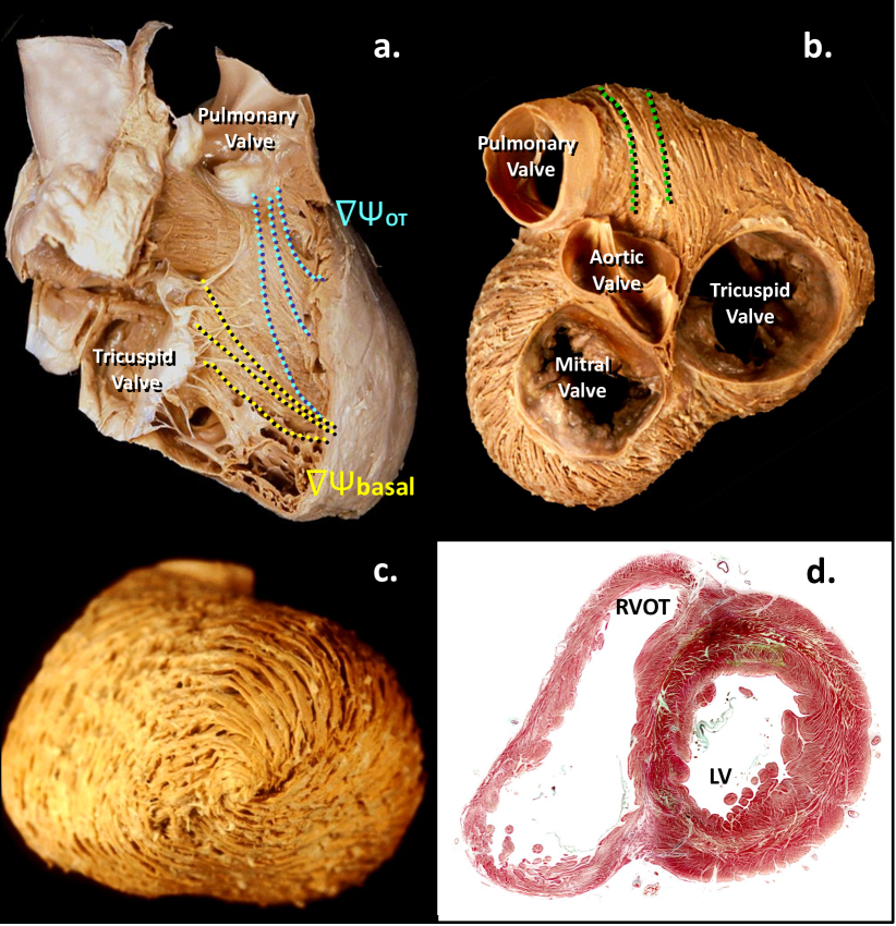
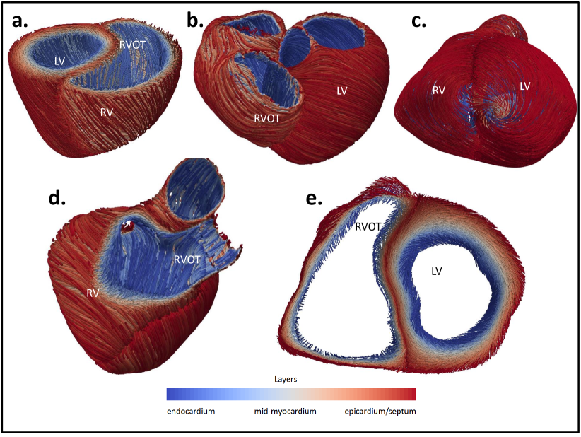
Refer to caption — Figure 1: Histological data of the heart. a) Fiber configuration in the RV sub- endocardium, with longitudinal directions to the pulmonary and tricuspid valves (dashed blue and yellow lines, respectively). b) Epicardial fiber configuration of both ventricles (top view). The dashed green line represent circumferential fibers of the OT. c) Apical view of the fiber epicardial layer d) Short axis slice of the heart showing transmural fiber orientation. $\nabla\Psi_{basal}$ : apico-basal direction; $\nabla\Psi_{OT}$ : apico-OT direction; RVOT: Right Ventricle Outflow Tract; LV: Left Ventricle

The two described strategies have the common issue of being mainly focused on the left ventricle (LV). This is due to the complexity of obtaining accurate data of the right ventricle (RV), especially on fiber orientation. For instance, according to histological data, fiber orientation in the RV sub-endocardium has a longitudinal direction from apex towards pulmonary and tricuspid valves, as illustrated in Figure 1, which is not the case in LV-based RBM. The outflow tract (OT) of the ventricles is a structure that plays a key role in some pathologies like outflow tract ventricular arrhythmia (OTVA). It has a particular fiber configuration with longitudinal and circumferential directions in the sub-endocardium and sub-epicardium, respectively. Unfortunately, most biventricular computational models include an artificial basal plane well below the valves rather than a complete biventricular geometry, thus not including the outflow tracts.

To overcome these issues, we have developed a RBM that includes specific fiber orientation in different cardiac regions such as the RV endocardium, the interventricular septum and the outflow tracts, following observations from histological data. This outflow tract extended RBM (OT-RBM) allows running in silico simulations modelling pathologies where these regions are relevant such as OTVAs and Tetralogy of Fallot, among others. The OT-RBM processes both ventricles independently, which gives more flexibility to generate different fiber configurations. Therefore, septal fiber orientation can also be independently modified, allowing the study of its discontinuity, which is still under debate [28, 29, 30]. In this work, the introduced RBM is compared with state-of-the-art fiber generation models such as the ones based on Streeter observations [23] and Bayer et al. [25], as well as with DT-MRI data. Additionally, electrophysiological simulations with fiber orientation provided by the OT-RBM are performed in a set of nine patient-specific OTVA biventricular geometries. Simulation results are then compared to clinical observations from electro-anatomical maps of these patients for different sites of origin of the ectopic focus.

2 Methods

2.1 General overview

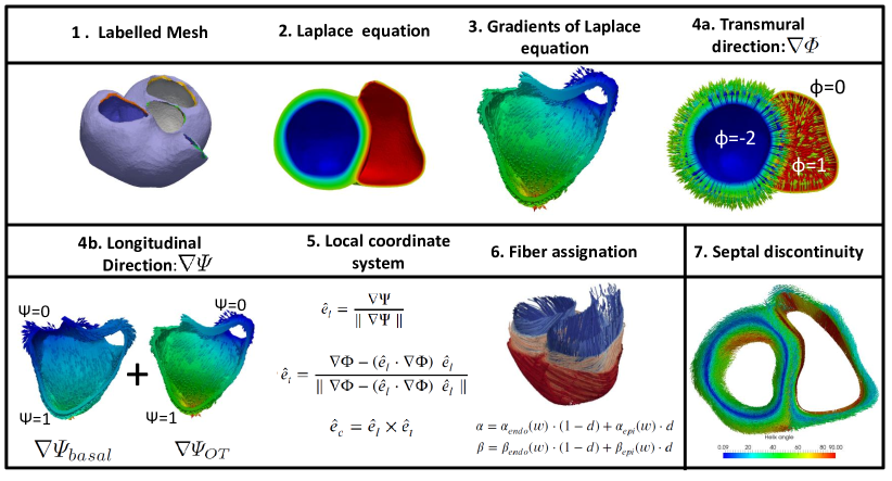
The OT-RBM uses the Laplace-Dirichlet method introduced in the work of Bayer et al. [25] (which is mainly based on LV fiber observations) to create a new local coordinate system in each point of the mesh. This coordinate system allow assigning specific fiber information in the RV according to histological data and extending it to the outflow tracts of both ventricles. Additionally, the proposed RBM allows, if necessary, septal fiber discontinuities between the LV and RV. The whole pipeline to develop the new RBM is summarized in Figure 2. It starts with the generation of volumetric labelled biventricular meshes, representing cardiac structures including outflow tracts from both ventricles up to the valve planes. Subsequently, the Laplace equation is solved with different boundary conditions to define the directions (i.e. transmural and longitudinal) required for the local coordinate system that will guide fiber assignment at each point of the mesh. The longitudinal direction in both ventricles is defined as a combination of the vector fields resulting from the Laplace equation between the apex and the two valves. Once the directions are computed, a local coordinate system is generated at each point of the mesh. Fiber orientation is finally estimated for each cardiac structure after finding the most appropriate angles of the coordinate system to match histological observations.

2.2 Volumetric labelled mesh generation

Biventricular geometries used in this work were represented by patient-specific tetrahedral meshes built from the processing of computed tomography (CT) images. These images corresponded to nine patients with idiopathic OTVAs submitted for ablation procedure at Hospital Clínic de Barcelona. A MDCT ECG-gated study was performed on a 128 x 2 -slice CT scanner (Somatom Definition Flash, Siemens Healthcare, Erlangen, Germany). Images were acquired during an inspiratory breath-hold using retrospective ECG-gating technique with tube current modulation set between 50% and 100% of the cardiac cycle. The isotropic spatial resolution was 0.4 x 0.4 x 0.4 mm.

The biventricular geometries, including the outflow tracts and valve planes, were obtained from CT images using a semi-automatic segmentation procedure with region growing techniques available in the 3DSlicer ¹¹1https://www.slicer.org software. Subsequently, surface meshes were generated from the obtained binary segmentations applying the classical Marching Cubes method, which was followed by some post-processing steps (e.g. smoothing, labelling) performed in Blender ²²2https://www.blender.org. Finally, tetrahedral meshes ( $\sim$ 80000 nodes and $\sim$ 400000 elements) were created using the iso2mesh ³³3http://iso2mesh.sourceforge.net tool.

The next step of the methodology was mesh labelling, where different cardiac geometrical surfaces were identified to apply the Dirichlet conditions and construct the local reference system. These surfaces were the epicardium, the RV and LV endocardial walls, RV and LV apices and the four heart valves. These regions were easy to identify in the studied CT images, enabling the application of the OT-RBM in a wide variety of heart geometries. Mesh labelling is usually performed either manually, by tagging surfaces during the segmentation process [31], or using semi-automatic techniques [25, 32]. We used a semi-automatic approach where the apices and valve position were manually selected in CT images and endocardial and epicardial surfaces were automatically identified using ray/triangle intersection algorithms [33]. Rays were traced from the normal of every face of the surface mesh and intersections with other faces were computed. If intersections were found, the face was classified as endocardium; the rest were set as epicardium. Figure 2 (Step 1) shows the resulting mesh labelling for one of the processed biventricular geometries. Each mesh region is identified by a different color.

2.3 Local coordinate system

Cardiac fibers in finite-element meshes are represented in each node by an unitary 3D vector that is oriented in the preferential direction of the electrical propagation and mechanical contraction of the myofiber. Therefore, a local orthonormal coordinate system is needed to define the myofiber vector in all mesh nodes. The orthotropic axes of the reference system are the longitudinal ( $\hat{e}_{l}$ ), transmural ( $\hat{e}_{t}$ ) and local circumferential ( $\hat{e}_{c}$ ) directions. Transmural and longitudinal directions can be defined by solving the Laplace equation using the corresponding surfaces as Dirichlet boundary conditions and computing the gradient of the solution, as in Bayer et al. [25]. In the OT-RBM these geometrical surfaces were the RV and LV endocardial walls, the whole bi-ventricular epicardium, the RV and LV apices and the four cardiac valves (the tricuspid and pulmonary valves for the RV and the mitral and aortic valves for the LV). The local circumferential direction was defined as the cross product of transmural and longitudinal directions. Fiber orientation was then obtained by rotating the obtained vector $\hat{e}_{c}$ by a given angle $\alpha$ and $\beta$ to match histological observations.

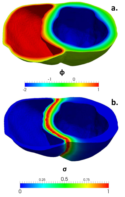
Transmural direction ( $\nabla\Phi$ ) was obtained by solving the Laplace equation between the endocardium of each ventricle and the epicardium; subsequently the gradient of the Laplace solution (Figure 3a) was computed. Negative and positive values were correspondingly assigned to the LV and RV endocardium ( $\Phi=-2$ and $\Phi=1$ , respectively) as Dirichlet boundary conditions. The epicardium was assigned to a zero value ( $\Phi=0$ ), thus allowing a discrimination between the two ventricles: positive and negative values were assigned to the RV and LV, respectively. These boundary conditions allowed to replicate findings from histological studies that affirm that two thirds of the septum belong to the LV and one third to the RV [13, 29, 34, 35]. Laplace equations and its gradients were solved using Elmer software ⁴⁴4https://www.csc.fi/web/elmer.

The longitudinal direction ( $\nabla\Psi$ ) was defined separately for each ventricle. This direction was the result of the weighted sum of the apico-basal ( $\nabla\Psi_{basal}$ ) and apico-OT ( $\nabla\Psi_{OT}$ ) gradients, defined individually in both ventricles: $\nabla\Psi_{basal}$ considered the apex-mitral valve and the apex-tricuspid valve directions in the LV and the RV, respectively; $\nabla\Psi_{OT}$ followed the apex-aortic valve and the apex-pulmonary valve directions in the LV and RV, respectively. These directions were already described by Greenbaum et al. [36] and can be visualized in Figure 1 (dashed lines). The resulting longitudinal fiber direction for each ventricle was set as follows:

\nabla\Psi=\nabla\Psi_{basal}\cdot w+\nabla\Psi_{OT}\cdot(1-w)

(1)

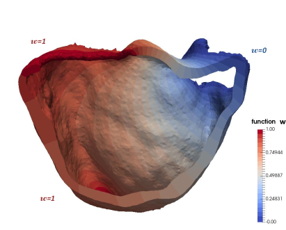
The sum of the apico-basal and apico-OT gradients was weighted by an intra-ventricular interpolation function $w$ , which was computed in the RV by solving the Laplace equation between the apex ( $w=1$ ), tricuspid valve ( $w=1$ ) and pulmonary valve ( $w=0$ ), as shown in Figure 4. In the LV, the equation was solved involving the apex ( $w=1$ ), the mitral valve ( $w=1$ ) and the aortic valve ( $w=0$ ). In this way, we obtained a smooth distribution of values following the cardiac surface allowing to properly define the OTs and control the smoothness in fiber changes near the OT in different geometries.

Using the previously calculated gradients ( $\nabla\Psi$ , $\nabla\Phi$ ), the local coordinate system was set up for each mesh node, which is fully described with the following vectors:

\displaystyle\hat{e}_{l}=\frac{\nabla\Psi}{\parallel\nabla\Psi\parallel}

\displaystyle\hat{e}_{t}=\frac{\nabla\Phi-(\hat{e}_{l}\cdot\nabla\Phi)\enskip\hat{e}_{l}}{\parallel\nabla\Phi-(\hat{e}_{l}\cdot\nabla\Phi)\enskip\hat{e}_{l}\parallel}\quad

\displaystyle\hat{e}_{c}=\hat{e}_{l}\times\hat{e}_{t}

(2)

2.3.1 Rotation of local coordinate system to match histological observations

Fiber orientation was finally obtained in every mesh node by rotating the local coordinate system to better match histological observations, as follows: 1) Vector $\hat{e}_{c}$ was rotated counterclockwise around $\hat{e}_{t}$ by an angle $\alpha$ ; and 2) subsequently, vector $\hat{e}_{c}$ was again rotated counterclockwise around $\hat{e}_{l}$ by a transverse angle $\beta$ . Note that the definition of angle $\alpha$ (angle with respect to the local circumferential direction) is not equivalent to the $\alpha$ helix angle defined in other histological studies or RBMs. The main reason is that our longitudinal direction is not always oriented in the apico-basal direction since it also has a component pointing in the apex-OT direction, which is the predominant one in the OTs. Far from the OTs, where the apex-OT component is negligible, the longitudinal direction only points towards the atrioventricular valves and therefore, our angle $\alpha$ and the helix angle match.

The first rotation was defined in each ventricle as a counterclockwise rotation of the vector $\hat{e}_{c}$ around $\hat{e}_{t}$ with an angle $\alpha$ :

\displaystyle\alpha=\alpha_{endo}(w)\cdot(1-d)+\alpha_{epi}(w)\cdot d

(3)

where $d$ is the transmural depth normalized from 0 to 1. The different values of $\alpha_{endo}$ and $\alpha_{epi}$ were chosen to replicate the following observations from several histological studies [10, 34, 36, 37]:

1.

Left ventricle (based on Greenbaum’s observations [36]): $\alpha_{endo}(w=1)=-60^{\circ}$ ; $\alpha_{epi}(w=1)=60^{\circ}$
2.

Right ventricle (based on Greenbaum [36], Ho [37] and Sanchez-Quintana [34]): $\alpha_{endo}(w=1)=90^{\circ}$ (same as longitudinal direction); $\alpha_{epi}(w=1)=-25^{\circ}$
3.

Outflow tracts (based on Sanchez-Quintana [34]): $\alpha_{epi}(w=0)=0^{\circ}$ (circumferential direction); $\alpha_{endo}(w=0)=90^{\circ}$ (longitudinal direction)

The expression for the transverse angle, $\beta$ , was the following:

\displaystyle\beta=\beta_{endo}(w)\cdot(1-d)+\beta_{epi}(w)\cdot d

(4)

Values of the transverse angle were derived from several studies [36, 38, 39] as follows:

1.

Left ventricle:

$\beta_{endo}(w=1)=-20^{\circ}$ and $\beta_{epi}(w=1)=20^{\circ}$
2.

Right ventricle:

$\beta_{endo}(w=1)=0^{\circ}$ and $\beta_{epi}(w=1)=20^{\circ}$
3.

Outflow tracts:

$\beta_{endo}(w=0)=0^{\circ}$ and $\beta_{epi}(w=0)=0^{\circ}$

2.3.2 Septal configuration

The OT-RBM allowed to control fiber angles in the septum, since we previously divided our septal geometry into RV and LV using the transmural direction. Therefore, the intersection surface between both ventricles (i.e. inter-ventricular septal surface) can be used to guide the interpolation of fiber angles in the septum. This is done by solving the Laplace equation between the inter-ventricular septal surface and the RV and LV endocardium (Figure 3, b). The obtained values ( $\sigma$ ) were used for forcing a smooth transition in both ventricles from the initial fibers in the septal surface ( $\alpha_{septal}$ ). Hence, the final expression for assigning the fiber angle in the septum, which could easily be modified to enforce continuity or a certain angle of discontinuity, was the following:

\displaystyle\alpha_{final}=\alpha\cdot(1-\sigma)+\alpha_{septal}\cdot\sigma

(5)

3 Experimental results

Results of applying the developed method to different geometries can be seen in Figure 5. They show a good agreement with histological data presented in Figure 1, especially in certain areas: right ventricle outflow tract (RVOT) fiber orientation (Figure 1a and Figure 5a, b, d); epicardial fiber configuration (Figure 1b, c and Figure 5b, c); and the transmural variation in LV fibers (Figure 1d and Figure 5e). A more exhaustive and quantitative evaluation of OT-RBM performance was conducted by means of three experiments, described below.

3.1 Experiments

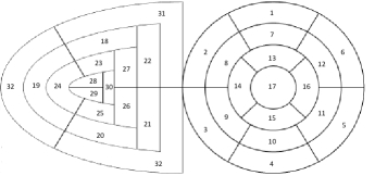
Three experiments were designed and conducted to analyze the performance of the proposed RBM. In the first experiment we estimated the differences between fiber configurations provided by the OT-RBM and existing ones in the literature. Magnetic resonance imaging data from an ex-vivo human heart available at the Johns Hopkins database ⁵⁵5http://cvrgrid.org/data/ex-vivo, which also includes fiber information from DT-MRI was used for this experiment. Differences were computed as the angle between fibers in each point of the mesh. Furthermore, mean angle differences were evaluated in different regions of the heart, dividing the LV into the 17 AHA regions according to the well-known description of Cerqueira et al. [40]. For the RV, a division in 15 regions based on the model proposed by Zhong et al. [41] was performed.

Table 1: Clinical ratio (Longitudinal/Perpendicular diameter) of the 10 ms isochrones map area obtained from the simulated OTVAs using different SOO and RBMs. (RVOT: right ventricle outflow tract; RCC: right coronary cusp; LCC: left coronary cusp; OT-RBM: Outflow Tract extended rule based method; ST-RBM: Streeter-Based rule based method)

Patient
		P1	P2	P3	P4	P5	P6	P7	P8	P9	All
	RVOT	2.06	1.59	2.07	2.15	1.81	1.70	1.78	1.99	1.55	1.86 $\pm$ 0.22
OT-RBM	LVOT-RCC	1.08	0.99	0.62	1.14	1.00	1.23	0.99	1.24	0.84	1.02 $\pm$ 0.2
	LVOT-LCC	0.46	0.41	0.73	0.56	0.76	0.95	0.79	0.78	0.75	0.74 $\pm$ 0.25
ST-RBM	RVOT	0.50	0.43	0.50	0.96	0.58	0.59	0.49	0.50	0.56	0.57 $\pm$ 0.16
	LVOT-RCC	0.87	0.77	0.42	0.95	1.70	1.31	1.14	1.35	1.08	1.07 $\pm$ 0.37
	LVOT-LCC	0.70	0.51	0.46	0.44	1.13	1.46	1.01	0.55	0.39	0.74 $\pm$ 0.4
Clinical		0.54 (RCC)	0.81 (LCC)	0.73 (RCC)	0.67 (LCC)	0.82 (RCC)	0.64 (RCC)	1.63 (RVOT)	0.71 (RCC)	2.27 (RVOT)

Since the previous geometry did not include detailed fiber information in the OTs, we performed a second experiment where OT fibers are indirectly compared. This experiment involved running electrophysiological simulations, including fiber orientation patterns computed with the OT-RBM and the Streeter-based one, on heart geometries from nine idiopathic OTVA patients. The simulated electrical propagation waves were then compared with clinical data from the OTVA patients, acquired during the ablation procedure at Hospital Clínic de Barcelona, Spain. Clinical data consisted of electro-anatomical maps acquired by the CARTO 3 system (Biosense Webster, Inc., Diamond Bar, CA, USA). Early activation sites were manually identified by clinicians during the intervention. Characteristics of the isochrones (area, axis ratio) around the earliest activated point in the RV endocardium were also manually measured by clinicians after the intervention. Isochronal characteristics provide useful information to predict the site of origin (SOO) of the ectopic focus [42, 43]: if the longitudinal axis of the isochrones follows the apico-basal axis, the SOO should be in the RVOT (following the fibers in the OT); while left ventricle outflow tract (LVOT) origins create more isotropic isochrones or with a larger perpendicular axis.

Simulations were performed with the SOFA software ⁶⁶6http://www.sofa-framework.org using the Mitchell-Schaeffer model [44] in patient-specific biventricular geometries. The SOO was placed in different parts of the OTs, including the one found by the clinicians during the intervention. Anisotropy conductivity ratio was set 2.5 in order to produce a higher conduction velocity along the fiber direction than in the transverse plane. The isochronal area, i.e. the surface occupied by mesh elements in the RV endocardium that has been activated at a given time (10 ms in our case) after the earliest activated point, and the clinical ratio of the simulated isochrones were calculated in each case following the same protocol than clinicians when analyzing isochrones from the electro-anatomical data [42, 43]. The protocol implemented by the clinicians measures the longitudinal diameter of the isochronal map area, which was defined by a line parallel to the septal projection of the RVOT longitudinal axis (perpendicular to the plane of the pulmonary valve). The defined longitudinal axis specified the perpendicular axis of the early activated area (perpendicular direction of the longitudinal axis).

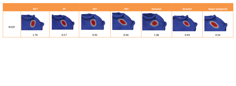
Finally, in order to demonstrate the influence of fiber orientation in electrophysiological simulations we carried out a sensitivity analysis by changing RVOT fiber orientation by different angles and performing simulations from two different SOO (RVOT and right coronary cusp). Resulting isochrones were evaluated and compared with clinical observations.

3.2 Comparison with other RBM and DT-MRI

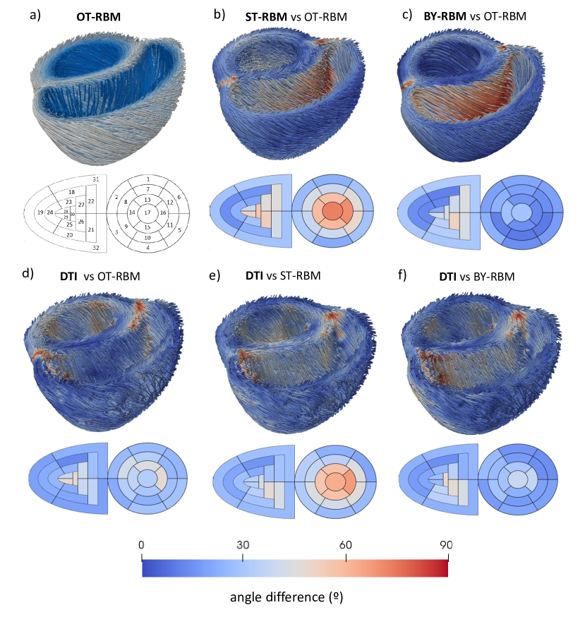
Figure 6 shows the comparison of fiber distribution maps provided by the OT-RBM, the one based on Streeter (ST-RBM) [45], Bayer et al. [25] (BY-RBM) and DT-MRI on the ex-vivo human heart from the Johns Hopkins database. The top row of the figure shows the fiber configurations provided by the OT-RBM, ST-RBM and BY-RBM models (a, b, c, respectively). The bottom row shows the comparison between DT-MRI fibers and the different RBMs: OT-RBM (d), ST-RBM (e) and BY-RBM (f). Information about the mean angle difference projected into a 2D visualization of different regions of the heart is also included in the figure. A quantitative analysis of these regional average angle differences is summarized in APPENDIX A. As expected, the main angle differences (red colors in Figure 6) between our model and the other RBMs are found in the RV endocardium, where we defined longitudinal directions from the apex towards the pulmonary and tricuspid valves. Fibers are more circumferential when generated with the other RBMs, when compared to histological data in this region. Low differences were found in the LV, especially comparing to BY-RBM (<20^∘). The comparison with BY-RBM also presented low differences in the free wall of the RV (<15^∘). Differences between OT-RBM and DT-MRI fibers are slightly larger in the LV ( $\sim$ 30^∘) but there is only one region, close to the apex, with high angle differences (>45^∘, region number 16). The ST-RBM and BY-RBM methods, especially the former, also present difficulties for generating fibers close to DT-MRI data in the LV apex (>60^∘ and $\sim$ 38^∘ for ST-RBM and BY-RBM, respectively).

3.3 Electrophysiological simulations on OTVA biventricular geometries

Isochrone ratios and areas were estimated for the electrophysiological simulations with RVOT and LVOT sites of origin using fiber directions computed with the OT-RBM and the ST-RBM. A quantitative analysis of isochrone ratios provided by electrophysiological simulations with the OT-RBM and the ST-RBM with different SOO in nine different patient-specific biventricular geometries is shown in Table 1. It also includes the SOO identified by the clinician and the manually measured isochrone ratio during the intervention. For each origin, mean of isochrone ratios were the following (mean $\pm$ SD): $1.86\pm 0.22$ and $0.57\pm 0.16$ for RVOT-SOO using OT-RBM and ST-RBM, respectively; and 0.88 $\pm$ 0.3 and 0.9 $\pm$ 0.4 for LVOT-SOO, using OT-RBM and ST-RBM respectively. We can observe than the largest differences correspond to RVOT-SOO, where the OT-RBM successfully predicted a larger longitudinal direction than the transversal one, unlike ST-RBM.

The obtained isochrone areas were the following (mean $\pm$ SD): 1.5 $\pm$ 0.4 cm² and 1.4 $\pm$ 0.4 cm² for RVOT-SOO using OT-RBM and ST-RBM, respectively; and 5.5 $\pm$ 2.3 cm² and 5.6 $\pm$ 2.1 cm² for LVOT-SOO using OT-RBM and ST-RBM, respectively. Therefore, both RBM provided similar results in terms of isochrone areas, independently of the site of origin.

We also evaluated the potential of the OT-RBM as a tool to predict the SOO in OTVAs. An example of differences between isochrones obtained in the RV endocardium around the earliest activated point from the electrophysiological simulations with different SOO can be seen in the first column of Figure 7. For LVOT origin we generated simulations from the right and left coronary cusps (RCC and LCC, respectively). Substantial differences were found in the isochrone characteristics depending on the site of origin, mainly a higher degree of isochronal isotropy with a LVOT origin (RCC in the figure) than with a RVOT origin, where the longitudinal direction along the fibers is preferential.

We can observe that the OT-RBM contributes to simulate isochrone ratios well differentiated depending on the RV or LV site of origin. A dependent t-test between results in statistically significant differences between isochrone ratios from RVOT-SOO and RCC-SOO ( $p<0.001$ ) and from RVOT-SOO and LCC-SOO ( $p<0.001$ ), but not from RCC-SOO and LCC-SOO. Additionally, the OT-RBM successfully replicated clinical findings such as the preferential longitudinal direction in RVOT origins (isochrone ratios larger than 1.5 in P7 and P9), unlike the Streeter-based one (isochrone ratios around 0.6 in P7 and P9).

3.4 Sensitivity analysis

A sensitivity analysis was carried out to assess the influence of RVOT fiber orientation in the simulated RV isochrones, with different ectopic focus in the RVOT and LVOT (RCC origin). Fibers were changed as follows: 90^∘ (chosen value in the OT-RBM), 0^∘, 45^∘ and -45^∘. We also included fiber configurations provided randomly, with ST-RBM and BY-RBM; we extended ST-RBM and BY-RBM to work in heart geometries with OT, placing the basal plane boundary condition in the mitral and tricuspid valves. Figure 7 shows the simulated 10 ms isochrones in the RV and their corresponding clinical isochrone ratio, obtained with the different fiber configurations. Longitudinal and perpendicular ratios are displayed in yellow and green arrows, respectively. Only simulations guided by OT-RBM generated fibers were able to replicate the high clinical ratio (1.78) and correct isochronal orientation obtained with a RVOT site of origin. The simulated isochrones with a LVOT-RCC origin did not present large differences with respect to the chosen fiber configuration.

4 Discussion

The aim of this work was to develop a novel rule-based method (OT-RBM) for assigning myofiber orientation in heart geometries including specific information of the RV and OTs. This new method will allow performing in silico studies to better understand and predict the behaviour of cardiac pathologies where the RV and OTs have an important role. The developed OT-RBM is based on myocyte aggregate configuration observed on histological data. It includes the following novel features that were not available before: 1) treatment of each ventricle separately, which improves the individual fitting of fiber angles; 2) new definition of longitudinal direction ( $\nabla\Psi$ ) based on histological descriptions [36, 37], which generate a new coordinate system allowing simple angle assignation to different regions of the heart; 3) fiber angles specific to the LV, RV, septum and OTs; and 4) addition of septal interpolation between the ventricles. These novelties make the OT-RBM flexible enough to assimilate fiber information from multimodal imaging (DT-MRI, histology, synchrotron data) and to work in a wide variety of heart geometries.

The proposed OT-RBM was compared with state-of-the-art RBMs, namely Streeter-based RBM (ST-RBM) and Bayer’s RBM (BY-RBM). Differences on fiber configuration provided by the different RBMs can be visualized in Figure 6. A quantitative regional comparison is also provided in Appendix A. As expected, the largest differences appear mainly near the RVOT, the RV endocardium and closer to the septum. For instance, ST-RBM and BY-RBM fibers are more circumferential that when generated with the OT-RBM, when compared to histological data in the RV. Interestingly, there were small differences (<20^∘) observed between OT-RBM and BY-RBM fiber configurations in the LV. This suggests that longitudinal directions obtained with the apex-mitral and apex-aortic valve boundary conditions in OT-RBM are equivalent to the apex-base ones in BY-RBM in the LV. The LV valve geometrical configuration, where the mitral and aortic valves are quite close together is probably the main reason for the OT-RBM and BY-RBM similarities in the LV. Over all the studied regions OT-RBM fibers were closer to BY-RBM ones, comparing to ST-RBM results.

The different RBMs were indirectly compared running electrophysiological simulations involving the outflow tracts guided by the different RBM-based fiber configurations. Results of this comparison can be seen in Figure 7. One of the major contributions of the OT-RBM is that it greatly improved OTVA simulations when compared to clinical observations. The simulated longitudinal/perpendicular clinical ratios of the isochrones (Table 1 and first column of Figure 7) were in agreement with measurements made by clinicians during the intervention [42]. According to this study, clinical ratios for RVOT isochrones are 1.9 $\pm$ 1.2 (n=14) and 0.79 $\pm$ 0.4 (n=23) for LVOT isochrones. The OT-RBM isochrone clinical ratio for RVOT cases in our simulation study (1.86 $\pm$ 0.22; see Table 1) was very close to the value measured by electrophysiologists. This agreement was possible due to the new distribution of fibers, especially in the RV and OTs, following histological observations. Other RBMs use simpler rules for generating fibers in these regions, obtaining unrealistic fiber configuration and, therefore, incorrect electric wave propagation and resulting isochrones (a ratio of 0.57 $\pm$ 0.16).

The influence of the fiber orientation in electrophysiological simulations was further analyzed in a sensitivity analysis (Figure 7). Isochrones obtained using the OT-RBM (90^∘) were the only ones showing good agreement with clinical observations from Electro-Anatomical Mapping (EAM) [42, 43]. When the origin of the arrhythmia is in the RVOT (top row of Figure 7), the longest axis is in the longitudinal direction of the RVOT, which corresponds to axis ratios larger than 1.5. By contrast, the remaining fiber configurations showed an isochronal principal direction opposite to clinical observations, as observed in Figure 7. Obtaining simulated isochrones similar to clinical ones by only following histological observations, while being blind to any other patient-specific electrophysiological data, is a strong feature of the proposed method.

Finally, we also compared the RBMs with fibers obtained from DT-MRI data. An ex-vivo human heart geometry from Johns Hopkins database was used for the comparison. Unfortunately, fiber orientation data was only available below a certain basal plane, substantially below the outflow tracts and the valves, preventing a detailed evaluation of the OT-RBM. Despite this limitation, the comparison showed relatively small fiber angle differences in the LV ( $\sim$ 30^∘; Figure 6,d), except close to the apex, which is a complex region for all RBMs when compared to DT-MRI data. The small fiber angle differences between OT-RBM, BY-RBM and DT-MRI data suggests that they will have a similar behavior in simulations involving the LV [1, 46, 47]. In the RV, differences to DT-MRI fibers obtained with the OT-RBM are slightly lower than the ones obtained with other RBMs, especially in the septum, which has high relevance in the OTVAs. It is important to highlight that the OT-RBM is not designed to strictly follow DT-MRI data (neither in the LV nor in the RV), but guided by histology-derived information. As can be seen in histological pictures shown in Figure 1, fibers in the RV endocardium and the OTs present a different orientation compared to those obtained by DT-MRI. The OT-RBM has been parameterized to match as much as possible fiber orientation observed in histological data and based on cardiac anatomist observations; by design, RV and OT fiber configuration from our RBM will necessarily differ from DT-MRI. Therefore, we cannot consider fiber angle differences between them as a conclusive index to assess the accuracy of the OT-RBM

Another major outcome of our study is the improved realism of OTVA electrophysiological simulations when guided by OT-RBM fiber configurations since it could support electrophysiologists in the prediction of the SOO in OTVA patients. Frequently, LVOT vs RVOT prediction of SOO in OTVAs is a challenging task for electrophysiologists, especially in difficult cases where the LVOT and RVOT geometries are spatially close and their electrophysiological signals from the electrocardiogram cannot be distinguished. Several works [42, 43, 48, 49] proposed several indices to predict the SOO of ectopic focus and then reduce the time of and improve the success rate of interventions. Using OT-RBM based electrophysiological simulations on patient-specific geometries, we have been able to differentiate the SOO by measuring the longitudinal/perpendicular clinical ratio of the 10 ms isochrones. According to Table 1 there are statistical significant differences between RVOT and LVOT (LCC or RCC) origin isochrone ratios. Isochronal areas can also be used to predict the SOO in simulations (larger in LVOT cases) but cannot be consistently be measured in clinical routine. The previous findings show the potential of our modelling pipeline to be used as an additional pre-operative source of information to the clinician to predict the site of origin of ectopic foci.

One of the main limitations of the method is the absence of quantitative 3D fiber information from imaging data in the RV and in the OTs. We developed our method being guided by findings in histological studies from 2D pictures of ex-vivo specimens and following recommendations from anatomists involved in this work. It would be desirable to compare our results with data obtained from advanced imaging techniques such as micro-CT or X-ray phase-contrast imaging, especially from the RV and OTs, which is rarely available in the literature. In this work we also compared our results with ex-vivo cardiac DT-MRI. This technique provides information related to myofiber orientation, but it cannot be considered as ground-truth since measurements are quite noisy, show poor signal-to-noise ratio and change under gradient calibration and temperature variation [50]. In addition, smoothing and interpolation techniques required to reconstruct tensor data from cardiac DT-MRI do not allow capturing myofiber orientation changes in very heterogeneous areas. Unlike in the LV, where DT-MRI may provide a good approximation of myofibers in most areas, this is particularly critical in thin structures of the heart such as the outflow tracts and the RV. Another limitation of the developed RBM is the smoothness of the resulting fiber orientation distributions, which is inherent to RBM. Unlike the variability found in histological data, RBM tend to generate idealistic fiber orientation, in part due to the use of too smooth biventricular geometries (e.g. without trabeculae). Finally, the definition of the longitudinal direction in some points of the boundary surfaces can affect the fiber orientation. Due to the definition of the boundary, the gradient in these points is zero, thus obtaining an incorrect fiber orientation (an example can be seen in Figure 6, where apical regions have a slightly higher angle difference in all cases). However, this problem can be minimized by reducing the number of points taken as boundaries and applying interpolation with the closest neighbors.

5 Conclusion

We have presented a RBM that includes fiber information specific to the RV, interventricular septum and both OT of the ventricles, to replicate histological observations. The proposed model facilitates the use of electrophysiological simulations in applications when these regions are important such as in OTVA patients, which was not possible before. The method has been indirectly validated comparing the results of electrophysiological simulations using fiber orientation provided by the proposed RBM with clinical observations in OTVA patients. These obtained results showed a very good agreement with clinical observations, demonstrating the potential of the developed modelling pipeline as a tool for the prediction of the site of origin of the ectopic focus in this type of arrhythmias. Further work will be focused on the application of this pipeline to a larger clinical database and in the adaptation of the developed RBM to high-resolution fiber information provided by X-ray phase-contrast imaging data.

6 Bibliography

References

[1] Arevalo Hermenegild J., Vadakkumpadan Fijoy, Guallar Eliseo, et al. Arrhythmia risk stratification of patients after myocardial infarction using personalized heart models. Nature Communications. 2016;7(May):11437.
[2] Lopez-Perez Alejandro, Sebastian Rafael, Ferrero Jose M. Three-dimensional cardiac computational modelling: methods, features and applications. BioMedical Engineering OnLine. 2015;14(1):35.
[3] Roberts DE, Hersh LT, Scher AM. Influence of Cardiac Fiber Orientation on Wavefront Voltage, Conduction Velocity, and Tissue Resistivity in the Dog. Circulation Research. 1979;44:701–712.
[4] Punske Bonnie B., Taccardi Bruno, Steadman Bruce, et al. Effect of fiber orientation on propagation: Electrical mapping of genetically altered mouse hearts. Journal of Electrocardiology. 2005;38(4 SUPPL.):40–44.
[5] Chen P S, Cha Y M, Peters B B, Chen L S. Effects of myocardial fiber orientation on the electrical induction of ventricular fibrillation.. The American journal of physiology. 1993;264(6 Pt 2):1760–73.
[6] Waldman L K, Nosan D, Villarreal F, Covell J W. Relation between transmural deformation and local myofiber direction in canine left ventricle. Circulation research. 1988;63(3):550–562.
[7] Lunkenheimer Paul P., Redmann Klaus, Westermann Philipp, et al. The myocardium and its fibrous matrix working in concert as a spatially netted mesh: a critical review of the purported tertiary structure of the ventricular mass. European Journal of Cardio-thoracic Surgery. 2006;29(SUPPL. 1):41–49.
[8] Smerup M., Partridge J., Agger P., et al. A mathematical model of the mechanical link between shortening of the cardiomyocytes and systolic deformation of the left ventricular myocardium. Technology and Health Care. 2013;21(1):63–79.
[9] Pluijmert Marieke, Delhaas Tammo, Parra Adrian Flores, Kroon Wilco, Prinzen Frits W., Bovendeerd Peter H M. Determinants of biventricular cardiac function: a mathematical model study on geometry and myofiber orientation. Biomechanics and Modeling in Mechanobiology. 2016;1–9.
[10] Sanchez-Quintana D., Garcia-Martinez V., Hurle J.M.. Myocardial Fiber Architecture in the Human Heart. Cells Tissues Organs. 1990;138(4):352–358.
[11] Scollan Df, Holmes a, Zhang J, Winslow Rl. Reconstruction of cardiac ventricular geometry and fiber orientation using magnetic resonance imaging. Annals of biomedical Enigneering. 2000;28(8):934–944.
[12] Jouk P S, Usson Y, Michalowicz G, Grossi L. Three-dimensional cartography of the pattern of the myofibres in the second trimester fetal human heart.. Anatomy and embryology. 2000;202(2):103–118.
[13] Gonzalez-Tendero Anna, Zhang Chong, Balicevic Vedrana, et al. Whole heart detailed and quantitative anatomy, myofibre structure and vasculature from X-ray phase-contrast synchrotron radiation-based micro computed tomography. European Heart Journal - Cardiovascular Imaging. 2017;:732–741.
[14] Varray François, Mirea Iulia, Langer Max, Peyrin Françoise, Fanton Laurent, Magnin Isabelle E.. Extraction of the 3D local orientation of myocytes in human cardiac tissue using X-ray phase-contrast micro-tomography and multi-scale analysis. Medical Image Analysis. 2017;38:117–132.
[15] Stephenson Robert S., Atkinson Andrew, Kottas Petros, et al. High resolution 3-Dimensional imaging of the human cardiac conduction system from microanatomy to mathematical modeling. Scientific Reports. 2017;7(1):7188.
[16] Toussaint Nicolas, Stoeck Christian T., Schaeffter Tobias, Kozerke Sebastian, Sermesant Maxime, Batchelor Philip G.. In vivo human cardiac fibre architecture estimation using shape-based diffusion tensor processing. Medical Image Analysis. 2013;17(8):1243–1255.
[17] Nielles-Vallespin Sonia, Mekkaoui Choukri, Gatehouse Peter, et al. In vivo diffusion tensor MRI of the human heart: Reproducibility of breath-hold and navigator-based approaches. Magnetic Resonance in Medicine. 2013;70(2):454–465.
[18] Deuster Constantin, Sammut Eva, Asner Liya, et al. Studying Dynamic Myofiber Aggregate Reorientation in Dilated Cardiomyopathy Using In Vivo Magnetic Resonance Diffusion Tensor Imaging.. Circulation. Cardiovascular imaging. 2016;9(10):e005018.
[19] Peyrat Jean Marc, Sermesant Maxime, Pennec Xavier, et al. A computational framework for the statistical analysis of cardiac diffusion tensors: Application to a small database of canine hearts. IEEE Transactions on Medical Imaging. 2007;26(10):1500–1514.
[20] Lombaert Herve, Peyrat Jean Marc, Croisille Pierre, et al. Statistical analysis of the human cardiac fiber architecture from DT-MRI. Lecture Notes in Computer Science (including subseries Lecture Notes in Artificial Intelligence and Lecture Notes in Bioinformatics). 2011;6666 LNCS:171–179.
[21] Lombaert Herve, Peyrat Jean Marc, Croisille Pierre, et al. Human atlas of the cardiac fiber architecture: Study on a healthy population. IEEE Transactions on Medical Imaging. 2012;31(7):1436–1447.
[22] Lekadir Karim, Hoogendoorn Corne, Pereanez Marco, Alba Xenia, Pashaei Ali, Frangi Alejandro F.. Statistical personalization of ventricular fiber orientation using shape predictors. IEEE Transactions on Medical Imaging. 2014;33(4):882–890.
[23] Streeter D D, Spotnitz Henry M, Patel Dali P, Ross J, Sonnenblick Edmund H. Fiber orientation in the canine left ventricle during diastole and systole.. Circulation research. 1969;24(3):339–347.
[24] Nielsen P. M., Le Grice I. J., Smaill B. H., Hunter P. J.. Mathematical model of geometry and fibrous structure of the heart.. The American journal of physiology. 1991;260(4 Pt 2):1365–1378.
[25] Bayer J. D., Blake R. C., Plank G., Trayanova N. A.. A novel rule-based algorithm for assigning myocardial fiber orientation to computational heart models. Annals of Biomedical Engineering. 2012;40(10):2243–2254.
[26] Wong Jonathan, Kuhl Ellen. Generating fibre orientation maps in human heart models using Poisson interpolation.. Computer methods in biomechanics and biomedical engineering. 2012;17(11):1217–26.
[27] Nagler Andreas, Gee Michael, Wall Wolfgang. Personalization of Cardiac Fiber Orientations from Image Data Using the Unscented Kalman Filter. FIMH. 2013;:132–140.
[28] Agger Peter, Stephenson Robert S., Dobrzynski Halina, et al. Insights from echocardiography, magnetic resonance imaging, and microcomputed tomography relative to the mid-myocardial left ventricular echogenic zone. Echocardiography. 2016;33(10):1546–1556.
[29] Boettler P, Claus P, Herbots L, et al. New aspects of the ventricular septum and its function: an echocardiographic study.. Heart (British Cardiac Society). 2005;91(10):1343–1348.
[30] Kocica Mladen J., Corno Antonio F., Carreras-Costa Francesc, et al. The helical ventricular myocardial band: global, three-dimensional, functional architecture of the ventricular myocardium. European Journal of Cardio-thoracic Surgery. 2006;29(SUPPL. 1).
[31] Crozier A., Augustin C. M., Neic A., et al. Image-Based Personalization of Cardiac Anatomy for Coupled Electromechanical Modeling. Annals of Biomedical Engineering. 2016;44(1):58–70.
[32] A. Palit S.K. Bhudia R. Wellings, Williams M.A.. Assigning Myocardial Fibre Orientation to a Computational Biventricular Human Heart Model. IFMBE Proceedings. 2014;43(January 2014):865–867.
[33] Möller Tomas, Trumbore Ben. Fast, Minimum Storage Ray/Triangle Intersection. Journal of Graphics Tools. 1997;2(1):21–28.
[34] Sanchez-Quintana Damian, Doblado-calatrava Manuel, Cabrera Jose Angel, Macías Yolanda, Saremi Farhood. Anatomical Basis for the Cardiac Interventional Electrophysiologist. BioMed Research International Ao. 2015.
[35] Agger P., Lakshminrusimha S., Laustsen C., et al. The myocardial architecture changes in persistent pulmonary hypertension of the newborn in an ovine animal model. Pediatric Research. 2016;79(4).
[36] Greenbaum R a, Ho S Y, Gibson D G, Becker a E, Anderson R H. Left ventricular fibre architecture in man.. British heart journal. 1981;45(July 1980):248–263.
[37] Ho S Y, Nihoyannopoulos P. Anatomy, echocardiography, and normal right ventricular dimensions.. Heart (British Cardiac Society). 2006;92 Suppl 1(C):i2-i13.
[38] Stephenson Robert S, Agger Peter, Lunkenheimer Paul P, et al. The functional architecture of skeletal compared to cardiac musculature ; myocyte orientation , lamellar unit morphology , and the helical ventricular myocardial band. Clinical Anatomy. .
[39] Lunkenheimer Paul P., Niederer Peter, Sanchez-Quintana Damian, Murillo Margarita, Smerup Morten. Models of ventricular structure and function reviewed for clinical cardiologists. Journal of Cardiovascular Translational Research. 2013;6(2):176–186.
[40] Cerqueira Manuel D, Weissman Neil J, Dilsizian Vasken, et al. Standardized Myocardial Segmentation and Nomenclature for Tomographic Imaging of the Heart. 2002;:539–542.
[41] Zhong L., Gobeawan L., Su Y., et al. Right ventricular regional wall curvedness and area strain in patients with repaired tetralogy of Fallot. AJP: Heart and Circulatory Physiology. 2012;302(6):H1306-H1316.
[42] Acosta Juan, Penela Diego, Herczku Csaba, et al. Impact of earliest activation site location in the septal right ventricular outflow tract for identification of left vs right outflow tract origin of idiopathic ventricular arrhythmias. Heart Rhythm. 2015;12(4):726–734.
[43] Herczku Csaba, Berruezo Antonio, Andreu David, et al. Mapping data predictors of a left ventricular outflow tract origin of idiopathic ventricular tachycardia with V3 transition and septal earliest activation.. Circulation. Arrhythmia and electrophysiology. 2012;5(3):484–91.
[44] Mitchell Colleen C, Schaeffer David G. A two-current model for the dynamics of cardiac membrane. Bulletin of mathematical biology. 2003;65(5):767–793.
[45] Sebastian R., Zimmerman V., Sukno F., Bijnens B.B., Frangi A.F. Cardiac Modelling for Pathophysiology Research and Clinical Applications. The Need for an Automated Pipeline. IFMBE Proceedings 2009 vol 25(4).
[46] Bayer J. D., Blake R. C., Plank G., Trayanova N. A.. A Novel Rule-Based Algorithm for Assigning Myocardial Fiber Orientation to Computational Heart Models. Annals of Biomedical Engineering. 2012;40(10):2243–2254.
[47] Deng Dongdong, Arevalo Hermenegild, Pashakhanloo Farhad, et al. Accuracy of prediction of infarct-related arrhythmic circuits from image-based models reconstructed from low and high resolution MRI. Frontiers in Physiology. 2015;6(OCT):1–12.
[48] Yoshida Naoki, Yamada Takumi, McElderry H. Thomas, et al. A novel electrocardiographic criterion for differentiating a left from right ventricular outflow tract tachycardia origin: The V2s/V3R index. Journal of Cardiovascular Electrophysiology. 2014;25(7):747–753.
[49] Zhang Fengxiang, Hamon David, Fang Zhen, et al. Value of a Posterior Electrocardiographic Lead for Localization of Ventricular Outflow Tract Arrhythmias: The V4/V8 Ratio. JACC: Clinical Electrophysiology. 2017;3(7):678–686.
[50] Teh Irvin, McClymont Darryl, Burton Rebecca A. B., et al. Resolving Fine Cardiac Structures in Rats with High-Resolution Diffusion Tensor Imaging. Scientific Reports. 2016;6(April):30573.