Numerical scattering for the defocusing Davey-Stewartson II equation for initial data with compact support

Abstract.

In this work we present spectral algorithms for the numerical scattering for the defocusing Davey-Stewartson (DS) II equation with initial data having compact support on a disk, i.e., for the solution of d-bar problems. Our algorithms use polar coordinates and implement a Chebychev spectral scheme for the radial dependence and a Fourier spectral method for the azimuthal dependence. The focus is placed on the construction of complex geometric optics (CGO) solutions which are needed in the scattering approach for DS. We discuss two different approaches: The first constructs a fundamental solution to the d-bar system and applies the CGO conditions on the latter. This is especially efficient for small values of the modulus of the spectral parameter $k$. The second approach uses a fixed point iteration on a reformulated d-bar system containing the spectral parameter explicitly, a price paid to have simpler asymptotics. The approaches are illustrated for the example of the characteristic function of the disk and are shown to exhibit spectral convergence, i.e., an exponential decay of the numerical error with the number of collocation points. An asymptotic formula for large $|k|$ is given for the reflection coefficient.

1. Introduction

Dispersive shock waves (DSW), i.e., zones of rapid modulated oscillations, appear in many applications in the vicinity of shocks whenever dispersion dominates dissipation. For the Korteweg-de Vries (KdV) equation, the seminal work by Gurevitch and Pitaevski [13] for step-like initial data provides analytic understanding of DSWs. The present work provides the first numerical step in the treatment of initial data with compact support for the Davey-Stewartson (DS) II equation,

(1) $$\begin{split}iq_{t}+(q_{xx}-q_{yy})+2\sigma(\Phi+|q|^{2})q&=0,\\ \Phi_{xx}+\Phi_{yy}+2(|q|^{2})_{xx}&=0,\end{split}$$

an integrable 2d nonlinear Schrödinger equation; here $\sigma=1$ in the defocusing case studied in the present paper, $\sigma=-1$ the in the focusing case. The reader is referred to [18] for a review on DS equations (also non-integrable cases) and a comprehensive list of references. We give numerical algorithms for the computation of the scattering transform for initial data with compact support on a disk for $\sigma=1$. We note here that, much like in the linear case of Fourier transformations, the direct and inverse problems are essentially the same.

1.1. D-bar systems

An asymptotic description of DSWs is in general only possible for small amplitudes via multiscales approximations. For completely integrable equations in one spatial dimension, steepest descent techniques for Riemann-Hilbert problems (RHPs) allow results for large amplitudes as well. A complete description of DSWs including the appearence of Painlevé transcendents exists so far only for the Korteweg-de Vries equation, see [11] for a review. For two-dimensional integrable equations d-bar problems often take the role RHPs play the 1d case, see [4]. For such problems no steepest descent techniques are known yet though partial progress has been made recently in [2] for the defocusing Davey-Stewartson II equation. In any case so far DSWs for two-dimensional integrable equations have been mainly studied numerically, see [19, 16, 17].

The direct scattering transformation for the DS II equations is given by a system of d-bar equations,

(2) $$\begin{array}[]{l}\bar{\partial}\psi_{1}=\frac{1}{2}q\psi_{2},\\ {}\\ \partial\psi_{2}=\frac{1}{2}\sigma\bar{q}\psi_{1},\end{array}$$

where the scalar functions $\psi_{1}$ and $\psi_{2}$ satisfy the complex geometric optics (CGO) asymptotic conditions

(3) $$\begin{array}[]{l}\lim_{|z|\to\infty}\psi_{1}\mathrm{e}^{-kz}=1,\\ {}\\ \lim_{|z|\to\infty}\psi_{2}\mathrm{e}^{-\bar{k}\bar{z}}=0;\end{array}$$

here $q=q(x,y,t)$ is a complex-valued field, the spectral parameter $k\in\mathbb{C}$ is independent of $z=x+\mathrm{i}y$, and

$$\partial:=\frac{1}{2}\left(\frac{\partial}{\partial x}-\mathrm{i}\frac{\partial}{\partial y}\right)\quad\text{and}\quad\bar{\partial}:=\frac{1}{2}\left(\frac{\partial}{\partial x}+\mathrm{i}\frac{\partial}{\partial y}\right).$$

The reflection coefficient $R=R(k)$ (which can be seen as a nonlinear analogue to a Fourier transform) is defined in terms of $\psi_{2}(z;k)$ as follows:

(4) $$\mathrm{e}^{-kz}\overline{\psi_{2}(z;k)}=\frac{1}{2}R(k)z^{-1}+O(|z|^{-2}),\quad|z|\to\infty.$$

The existence and uniqueness of CGO solutions to system (2) with $\sigma=1$ was studied in [29, 30]) for Schwartz class potentials and in [7, 5, 27, 25] for more general potentials. Note that the understanding is much less complete in the focusing case $\sigma=-1$ since the system (2) no longer has generically a unique solution for large classes of potentials $q$ for all $k\in\mathbb{C}$. There can be so-called exceptional points (special values of the spectral parameter $k$) where the system is not uniquely solvable. Note that the codes presented in this paper can also be applied to the focusing case in the absence of such exceptional points. However, since it is not clear when these points appear and since numerical problems are expected in the vicinity of exceptional points, we concentrate on the defocusing case here.

Systems of the form (2) also appear in electrical impedance tomography (EIT) in 2d, the reconstruction of the conductivity in a given domain from measurements of the electrical current through its boundary, induced by an applied voltage, i.e., from the Dirichlet-to-Neumann map. This problem was first posed by Calderon [8] and bears his name. For a comprehensive review of the mathematical aspects and advances see [32]. They also appear in the context of 2d orthogonal polynomials, and of Normal Matrix Models in Random Matrix Theory, see e.g. [12].

As $q$ in (1) evolves in time $t$ according to (1), the reflection coefficient evolves by a trivial phase factor:

(5) $$R(k;t)=R(k,0)e^{4it\Re(k^{2})}.$$

The inverse scattering transform for DS II is then given by (3) after replacing $q$ by $R$ and vice versa, the derivatives with respect to $z$ by the corresponding derivatives with respect to $k$, and asymptotic conditions for $k\to\infty$ instead of $z\to\infty$.

1.2. Numerical appoaches

Numerical approaches to d-bar systems have so far mainly taken the following path: the inverse of the d-bar operator is known to be given by the solid Cauchy transform

(6) $$\overline{\partial}^{-1}F(x,y):=-\frac{1}{\pi}\int\int_{\mathbb{R}^{2}}\frac{F(x^{\prime},y^{\prime})\,dx^{\prime}dy^{\prime}}{(x^{\prime}-x)+\mathrm{i}(y^{\prime}-y)},$$

a weakly singular integral. This integral can be either computed via finite difference, finite element discretizations, or via a Fourier approach, see [24] for a review of techniques.

The original approach [21], see also [3], uses a Fourier method for the computation of the integral, i.e., a 2d discrete Fourier transform. A rather bold regularization of the singular integrand was implemented by replacing the singularity simply by a finite value. This leads to a finite, but discontinuous integrand. Though discrete Fourier transforms are spectral methods which are known to show spectral convergence, i.e. an exponential decrease of the numerical error with the resolution, for the approximation of smooth functions, they are of first order method if a non-continuous function approximated. This means that the numerical error decreases only linearly with $1/N$ where $N$ is the number of Fourier modes. This first order convergence was proven in [21].

The first Fourier approach with spectral convergence (i.e., exponential decrease of the numerical error with the number $N$ of Fourier modes) was presented in [12] for potentials in the Schwartz class of rapidly decreasing smooth potentials $q$. The approach uses an analytic (up to numerical precision) regularization of the integrand. This is further developed in [15]. In practice this means that accuracies of the order of machine precision can be reached on low-cost computers which are out of reach of a first order method.

In various applications, treating potentials with compact support is crucial. The focus of this paper will be on such potentials. The method of [12] cannot be generalized to potentials with compact support without severe loss of spectral accuracy since Gibbs phenomena appear at the discontinuity, see for example [3] where a Fourier solver for the Beltrami equation is applied to various step like potentials. Therefore, here we present a completely different approach starting from a formulation of the system (2) in polar coordinates. The system is discretized with a Chebychev spectral method in the radial coordinate $r$ and a Fourier spectral method in the angular coordinate $\phi$. This means that the functions $\psi_{1,2}$ in (2) will be approximated via truncated series of Chebychev polynomials in $r$ and truncated Fourier series in $\phi$. Fast, efficient algorithms exist for both these approaches, making them a prime choice. In addition they are known to show an exponential decrease of the numerical error with the number of Chebychev polynomials and Fourier modes for smooth functions, i.e., here for smooth potentials $q$ on the disk. We show at examples that no Gibbs phenomena can be observed in our approach since we only approximate smooth functions (the functions are smooth on the considered domain, discontinuities appear only on the boundary). The numerical errors we discuss are thus always global, even at the discontinuity of the potential.

This discretization will be used in two different ways: First we construct a fundamental system of solutions to the finite dimensional system of ordinary differential equations (ODEs) with which (2) is approximated after discretization in $\phi$. Note that the discontinuity of $q$ at the boundary of the disk does not affect the method since the latter is a domain boundary. Smoothness is only required inside the computational domain. The approach can be applied for arbitrary $k$ since the system (2) is independent of the spectral parameter $k$. The CGO conditions (3) are then implemented for given values of $k$ by imposing them on this fundamental solution. It is shown that this works well for values of $|k|\lesssim 1$.

For larger $|k|$, cancellation errors will play a role in this approach. To address this, we introduce functions $\Phi_{1}=\mathrm{e}^{-kz}\psi_{1}$ and $\Phi_{2}=\mathrm{e}^{-\bar{k}\bar{z}}\psi_{2}$ which satisfy with (3) the simpler asymptotic conditions

(7) $$\lim_{|z|\to\infty}\Phi_{1}=1,\quad\lim_{|z|\to\infty}\Phi_{2}=0.$$

In other words, $\Phi_{1}$ and $\Phi_{2}$ are bounded functions at infinity. In terms of $\Phi_{1}$ and $\Phi_{2}$ the d-bar system (2) leads to

$$\begin{array}[]{l}\bar{\partial}\Phi_{1}=\frac{1}{2}q\mathrm{e}^{\bar{k}\bar{z}-kz}\Phi_{2},\\ {}\\ \partial\Phi_{2}=\frac{1}{2}\bar{q}\mathrm{e}^{kz-\bar{k}\bar{z}}\Phi_{1},\end{array}$$

for $\Phi_{1}$, $\Phi_{2}$ which contains the spectral parameter explicitly. The latter is solved with the same Chebychev and Fourier discretization as before, but this time with a fixed point iteration. This iteration is shown to converge rapidly in examples for all $k$ which allows to treat efficiently large values of $|k|$ and thus rapidly oscillating solutions.

The paper is organized as follows: In Section 2 we give analytical justification of the equations we are going to treat numerically using polar coordinates and study the example of $q$ being the characteristic function of the disk. In Section 3 we summarize the numerical schemes employed to discretize the differential operators and construct a fundamental solution to (2). This fundamental solution is used in Section 4 to construct CGO solutions. In Section 5 we apply a fixed point iteration to solve system (17) which is equivalent to (2). In Section 6 we add some concluding remarks.

2. D-bar system with compactly supported potentials on a disk

In this section we formulate the defining equations (2) and (3) for the CGO solutions in polar coordinates and use Fourier series in the azimuthal variable for the solutions. As an example we consider the case of constant potential on the disk.

2.1. Polar coordinates

We write $z=r\mathrm{e}^{\mathrm{i\phi}}$ in which (2) reads

(8) $$\begin{array}[]{l}\mathrm{e}^{\mathrm{i}\phi}\left(\partial_{r}+\frac{\mathrm{i}}{r}\partial_{\phi}\right)\psi_{1}=q(r,\phi)\psi_{2},\\ {}\\ \mathrm{e}^{-\mathrm{i}\phi}\left(\partial_{r}-\frac{\mathrm{i}}{r}\partial_{\phi}\right)\psi_{2}=\bar{q}(r,\phi)\psi_{1}.\end{array}$$

We are looking for solutions in the form of a Fourier series,

(9) $$\psi_{1}=\sum_{n\in\mathbb{Z}}a_{n}(r)\mathrm{e}^{\mathrm{i}n\phi},\quad\psi_{2}=\sum_{n\in\mathbb{Z}}b_{n}(r)\mathrm{e}^{\mathrm{i}n\phi}.$$

The functions $a_{n}$ and $b_{n}$ are determined by (8) for given $q(r,\phi)$ together with a regularity condition at $r=0$ up to a certain number of constants $\alpha_{n}$ and $\beta_{n}$ corresponding to general holomorphic respectively antiholomorphic functions arising in the determination of $a_{n}$ and $b_{n}$ respectively: if $a_{n}$ and $b_{n}$ are solutions to (8) regular for $r\to 0$, so are

(10) $$a_{n}(r)+\alpha_{n}r^{n},\quad n=0,1,2,\ldots,\quad b_{n}(r)+\beta_{n}r^{n},\quad n=0,-1,-2,\ldots$$

The constants $\alpha_{n}$, $\beta_{n}$ will be uniquely determined by the asymptotic conditions (3).

For $r>1$, where $q\equiv 0$, the function $\psi_{1}$ is a holomorphic function, whereas $\psi_{2}$ is antiholomorphic. Continuity of the functions at the disk thus implies for $r>1$

$$\psi_{1}=\sum_{n\in\mathbb{Z}}a_{n}(1)r^{n}\mathrm{e}^{\mathrm{i}n\phi},\quad\psi_{2}=\sum_{n\in\mathbb{Z}}b_{n}(1)r^{-n}\mathrm{e}^{\mathrm{i}n\phi}.$$

The first of the asymptotic conditions (3) is equivalent to $c_{0}=1$ and $c_{n}=0$ for $n>0$ for $r\to\infty$, where

(11) $$\sum_{n\in\mathbb{Z}}c_{n}r^{n}\mathrm{e}^{\mathrm{i}n\phi}:=\sum_{n=0}^{\infty}\sum_{m=0}^{n}\frac{(-k)^{m}}{m!}\left(a_{n-m}(1)r^{n}\mathrm{e}^{\mathrm{i}n\phi}+a_{m-n-1}(1)r^{2m-n-1}\mathrm{e}^{\mathrm{i}(2m-n-1)\phi}\right).$$

Since the conditions are imposed for $r\to\infty$, negative powers of $r$ in (11) can be neglected. This implies that there will be only conditions for the positive frequencies $c_{n}$, $n\geq 0$, which can be written in the form,

(12) $$c_{n}=\sum_{m=0}^{\infty}a_{n-m}(1)\frac{(-k)^{m}}{m!}.$$

Note that these conditions — though obtained in the limit $r\to\infty$ — lead here to conditions at the rim of the disk $r=1$ because of the holomorphicity of $\psi_{1}$ for $r>1$ and the continuity of the function at the rim of the disk. In other words, the solution in the exterior of the disk follows from the holomorphicity of $\psi_{1}$ there as well as the asymptotic condition and the continuity at the disk. It is not necessary to solve a PDE there in contrast to the disk. The convolutions in (12) can be computed in a standard way via Fourier series,

(13) $$c_{n}=\frac{1}{2\pi}\int_{0}^{2\pi}\mathrm{d}\phi\exp\left(-k\mathrm{e}^{\mathrm{i\phi}}\right)\sum_{m\in\mathbb{Z}}a_{m}(1)\mathrm{e}^{\mathrm{i(m-n)\phi}}.$$

In the numerical approach we present in Section 4, we will use the asymptotic conditions in the form (13).

Similarly we get for the second condition in (3) that $d_{n}=0$ for $n=0,-1,-2,\ldots$, where

$$\sum_{n\in\mathbb{Z}}d_{n}r^{n}\mathrm{e}^{\mathrm{i}n\phi}:=\sum_{n=0}^{\infty}\sum_{m=0}^{n}\frac{(-\bar{k})^{m}}{m!}\left(b_{n-m+1}(1)r^{2m-n-1}\mathrm{e}^{\mathrm{i}(n+1-2m)\phi}+b_{m-n}(1)r^{n}\mathrm{e}^{-\mathrm{i}n\phi}\right)$$

i.e.,

$$d_{n}=\sum_{m=0}^{\infty}b_{m-n}(1)\frac{(-\bar{k})^{m}}{m!}$$

This is equivalent to

(14) $$d_{n}=\frac{1}{2\pi}\int_{0}^{2\pi}\mathrm{d}\phi\exp\left(-\bar{k}\mathrm{e}^{\mathrm{-i\phi}}\right)\sum_{m\in\mathbb{Z}}b_{m}(1)\mathrm{e}^{\mathrm{i(n-m)\phi}}.$$

In this approach the reflection coefficient (4) is simply given by the coefficient $d_{1}$,

(15) $$R=2\bar{d}_{1}.$$

System (2) has the advantage that it is independent of the spectral parameter $k$. A disadvantage from a numerical point of view are the asymptotic conditions (3) which imply that the functions $\psi_{1}$ and $\psi_{2}$ have essential singularities at infinity. An alternative way to treat (2) is thus to introduce the functions

(16) $$\Phi_{1}=\mathrm{e}^{-kz}\psi_{1},\quad\Phi_{2}=\mathrm{e}^{-\bar{k}\bar{z}}\psi_{2},$$

which satisfy the asymptotic conditions (7). In the case of a potential $q$ with compact support, $\Phi_{1}$ is holomorphic in the complement of the support of $q$ and $\Phi_{2}$ is antiholomorphic there. System (8) for the functions (16) reads

(17) $$\begin{array}[]{l}\mathrm{e}^{\mathrm{i}\phi}\left(\partial_{r}+\frac{\mathrm{i}}{r}\partial_{\phi}\right)\Phi_{1}=q(r,\phi)\mathrm{e}^{\bar{k}\bar{z}-kz}\Phi_{2},\\ {}\\ \mathrm{e}^{-\mathrm{i}\phi}\left(\partial_{r}-\frac{\mathrm{i}}{r}\partial_{\phi}\right)\Phi_{2}=\bar{q}(r,\phi)\mathrm{e}^{kz-\bar{k}\bar{z}}\Phi_{1}.\end{array}$$

This system contains, in contrast to (8), not just $k$ but (for $|k|$ large) rapidly oscillating functions. On the other hand, the asymptotic conditions (7) are considerably simpler than the conditions (3). Therefore we will use (8) for values of $|k|\lesssim 1$, and (17) for larger values of $|k|$.

2.2. Example

In order to illustrate the above approach and to have a concrete example to test at least parts of the code, we consider the case of a constant potential at the disk,

$$q=\begin{cases}1,&r\leq 1\\ 0,&r>1\end{cases}.$$

Differentiating the first equation of (2) with respect to $\partial$ and eliminating $\psi_{2}$ via the second, we get in polar coordinates for $r\leq 1$

$$\partial_{rr}\psi_{1}+\frac{1}{r}\partial_{r}\psi_{1}+\frac{1}{r^{2}}\partial_{\phi\phi}\psi_{1}=\psi_{1}.$$

Note that the same equation holds for $\psi_{2}$. With (9), we get that the $a_{n}$ satisfy the modified Bessel equation

$$a_{n}^{\prime\prime}+\frac{1}{r}a_{n}^{\prime}-\frac{r^{2}+n^{2}}{r^{2}}a_{n}=0,$$

i.e., the solution regular on the disk is given by $a_{n}=\alpha_{n}I_{n}(r)$, where the $\alpha_{n}=const$ and where the $I_{n}(r)$ are the modified Bessel functions [1]. Thus we have for $r\leq 1$

(18) $$\psi_{1}=\sum_{n\in\mathbb{Z}}\alpha_{n}I_{n}(r)\mathrm{e}^{\mathrm{i}n\phi}.$$

For $r\leq 1$, the function $\psi_{2}$ can be computed from the first relation of (2). Because of the identity $I_{n}^{\prime}(r)-(n/r)I_{n}=I_{n+1}$, it can be written in the form

(19) $$\psi_{2}=\sum_{n\in\mathbb{Z}}\alpha_{n}\mathrm{e}^{\mathrm{i}(n+1)\phi}I_{n+1}(r).$$

For $r>1$, because of the continuity of the potentials at $r=1$ we get

(20) $$\psi_{1}=\sum_{n\in\mathbb{Z}}\alpha_{n}I_{n}(1)z^{n},\quad\psi_{2}=\sum_{n\in\mathbb{Z}}\frac{\alpha_{n}}{\bar{z}^{n+1}}I_{n+1}(1).$$

The constants $\alpha_{n}$, $n\in\mathbb{Z}$ are determined by the asymptotic condition (3). We only found an explicit solution for $k=0$, $\alpha_{0}=1/I_{0}(1)$ whereas $\alpha_{n}=0$ for $n\neq 0$. This implies

$$\psi_{1}=\begin{cases}I_{0}(r)/I_{0}(1),&r\leq 1\\ 1,&r>1\end{cases},$$

and

$$\psi_{2}=\begin{cases}I_{1}(r)/I_{0}(1)\mathrm{e}^{\mathrm{i}\phi},&r\leq 1\\ I_{1}(1)/I_{0}(1)/\bar{z},&r>1\end{cases},$$

3. Numerical construction of a fundamental solution to the d-bar system

In this section we present a spectral approach to the system (8) based on a discrete Fourier approach in $\phi$ and a Chebychev spectral method in $r$. We construct solutions $\psi_{1,2}^{(j)}$ to the system characterized by boundary conditions on the Fourier coefficients (9) at the rim of the disk, in a way that a basis of solutions is obtained. In the next section this system of fundamental solutions is subjected to the asymptotic conditions (13) and (14). The solutions are then tested for the example of subsection 2.2.

3.1. Spectral approach

The periodicity in the coordinate $\phi$ in (8) suggests to use Fourier techniques for this variable. This means that the series in (9) are approximated via discrete Fourier transforms which implies the use of a discrete variable $\phi$ sampled on the $N_{\phi}$ collocation points

$$\phi_{j}=\frac{2\pi j}{N_{\phi}},\quad j=0,1,\ldots,N_{\phi}-1$$

where $N_{\phi}$ is an even positive integer. Note that the discrete Fourier series is not only periodic in $\phi$, but also in the dual variable $n$. Since the d-bar system (8) contains factors $\mathrm{e}^{\pm\mathrm{i}\phi}$, we use an asymmetric definition of the Fourier sums approximating (9),

(21) $$\psi_{1}\approx\sum_{n=-N_{\phi}/2}^{N_{\phi}/2-1}a_{n}(r)\mathrm{e}^{\mathrm{i}n\phi},\quad\psi_{2}\approx\sum_{n=-N_{\phi}/2+1}^{N_{\phi}/2}b_{n}(r)\mathrm{e}^{\mathrm{i}n\phi},$$

in order to be able to deal with the same powers of $\mathrm{e}^{\mathrm{i}\phi}$ in both equations (we use the same symbols as in (8) to avoid cluttered notation). The discrete Fourier transforms can be computed conveniently with a Fast Fourier Transform (FFT).

With (21), the partial differential equation (PDE) system (8) is approximated via a finite system of ordinary differential equations (ODE) in $r$ for the $2N_{\phi}$ functions $a_{n}(r)$, $n=-N_{\phi}/2,\ldots,N_{\phi}/2-1$, and $b_{n}(r)$, $n=-N_{\phi}/2+1,\ldots,N_{\phi}/2$. To solve this system, we approximate these functions via a sum of Chebychev polynomials $T_{m}(l):=\cos(m\arccos x)$, $l\in[-1,1]$, i.e.,

(22) $$\begin{array}[]{l}a_{n}(r)\approx\sum_{m=0}^{N_{r}}a_{nm}T_{m}(l),\quad n=-\frac{N_{\phi}}{2},\ldots,\frac{N_{\phi}}{2}-1,\\ {}\\ b_{n}(r)\approx\sum_{m=0}^{N_{r}}b_{nm}T_{m}(l),\quad n=-\frac{N_{\phi}}{2}+1,\ldots,\frac{N_{\phi}}{2},\end{array}$$

where $r=(1+l)/2$. The constants $a_{nm}$ are determined via a collocation method: on the points

$$l_{j}=\cos\left(\frac{j\pi}{N_{r}}\right),\quad j=0,\ldots,N_{r}$$

the equations (22) are imposed as equalities, i.e., for fixed $n$ we have

$$a_{n}(r(l_{j}))=\sum_{m=0}^{N_{r}}a_{nm}T_{m}(l_{j}),\quad j=0,\ldots,N_{r}$$

which uniquely determines the $a_{nm}$. In the same way the $b_{nm}$ are fixed. Because of the definition of the Chebychev polynomials, one has $T_{m}(l_{j})=\cos(mj\pi/N_{r})$. Thus the coefficients $a_{nm}$ and $b_{nm}$ can be obtained via a Fast Cosine Transformation (FCT) which is related to the FFT, see e.g., the discussion in [31] and references therein.

The existence of fast algorithms, however, is not the only advantage of the Chebychev spectral method and the discrete Fourier transform. Both are so-called spectral methods which means that the numerical error in approximating smooth functions decreases faster than any power of $1/N_{r}$ and $1/N_{\phi}$, in practice it decreases exponentially. This is due to an analogue for discrete Fourier transforms of the well known theorem that the Fourier transform of a smooth, rapidly decreasing function is rapidly decreasing, see the discussion in [31].

To approximate derivatives via the ansatz (22), one uses $T_{0}^{\prime}(l)=0$, $T_{1}^{\prime}(l)=1$ and for $n\geq 1$ the identity

$$\frac{T^{\prime}_{n+1}(l)}{n+1}-\frac{T^{\prime}_{n-1}(l)}{n-1}=2T_{n}(l)$$

which implies that the derivative of the $a_{n}(r)$ is approximated via the action of a differentiation matrix $D$ on the Chebychev coefficients $a_{nm}$

$$a_{n}^{\prime}(r)\approx\sum_{m,\alpha=0}^{N_{r}}D_{m\alpha}a_{n\alpha}T_{m}(l)$$

The differentiation matrix is upper triangular and for even $N_{r}$ of the form

$$D=\begin{pmatrix}0&1&0&3&0&5&\ldots&N_{r}-1&0\\ &&4&0&8&\ldots&&&2*N_{r}\\ &&&6&0&10&\ldots&2*(N_{r-1})&0\\ &&&&8&0&12&\ldots&2*N_{r}\\ &&&&&\ddots&&&0\\ &&&&&&&&\vdots\\ &&&&&&&&0\\ &&&&&&&&2*N_{r}\end{pmatrix}.$$

In a similar way one can divide in the space of Chebychev coefficients by $r$ which is normally numerically a very delicate operation if $r$ can vanish on the considered interval as it does here. Using the identity

(23) $$T_{n+1}(l)+T_{n-1}(l)=2lT_{n}(x),\quad n=1,2,\ldots,$$

we can divide in coefficient space by $l\pm 1$. For given Chebyshev coefficients $a_{nm}$ we define the coefficients $\tilde{a}_{nm}$ via $\sum_{n=0}^{\infty}a_{nm}T_{m}(l)=:\sum_{n=0}^{\infty}(l\pm 1)\tilde{a}_{nm}T_{m}(l)$. This implies the action of a matrix $R$ in coefficient space (if $a_{n}(r)/r$ is bounded for $r\to 0$),

(24) $$\frac{a_{n}(r)}{r}\approx\sum_{m,\alpha=0}^{N_{r}}R_{m\alpha}a_{n\alpha}T_{m}(l).$$

The matrix $R^{-1}$ has for even $N_{r}$ the form

$$R^{-1}=\begin{pmatrix}1&1/2&&&\\ 1&1&1/2&&\\ &1/2&\ddots&\ddots&\\ &&\ddots&&\\ &&&&&1/2\\ &&&&1/2&1\end{pmatrix};$$

(the matrix $R$ is computed by inverting this matrix).

Denoting the combined action of FFT and FCT on a function $\psi(r,\phi)$ by $\mathbb{F}$, we thus approximate the system (8) via ($m=0,\ldots,N_{r}$)

$$\sum_{\alpha=0}^{N_{r}}\left(D-nR\right)_{m\alpha}a_{n\alpha} =\mathbb{F}\left(q(r,\phi)\mathrm{e}^{-\mathrm{i}\phi}\sum_{\alpha=0}^{N_{r}}\sum_{\beta=-N_{\phi}/2}^{N_{\phi}/2-1}b_{\beta\alpha}T_{\alpha}(l)\mathrm{e}^{\mathrm{i}\beta\phi}\right)_{nm},\quad n=-N_{\phi}/2,\ldots,N_{\phi}/2-1$$

(25) $$\sum_{\alpha=0}^{N_{r}}\left(D+nR\right)_{m\alpha}b_{n\alpha} =\mathbb{F}\left(\bar{q}(r,\phi)\mathrm{e}^{\mathrm{i}\phi}\sum_{\alpha=0}^{N_{r}}\sum_{\beta=-N_{\phi}/2}^{N_{\phi}/2-1}a_{\beta\alpha}T_{\alpha}(l)\mathrm{e}^{\mathrm{i}\beta\phi}\right)_{nm},\quad n=-N_{\phi}/2+1,\ldots,N_{\phi}/2.$$

The action of the functions $q(r,\phi)\mathrm{e}^{-\mathrm{i}\phi}$ and its conjugate in (25) is computed as a convolution in coefficient space via (23) and by using the periodicity of the FFT in Fourier space. Note that the computation of convolutions or products in a spectral method can lead to so called aliasing errors, see the discussion in [31], which are due to the fact that only a finite number of terms are considered in the Chebychev and Fourier sums, whereas for instance relation (23) implies the use of the whole series in order to get equality.

Denoting the vector built from the coefficients $a_{nm}$ by $A$ and the vector built by the coefficients $b_{nm}$ by $B$, equation (25) can be formally written as

(26) $$\mathcal{O}\begin{pmatrix}A\\ B\end{pmatrix}=0,$$

where $\mathcal{O}$ is the $2(N_{r}+1)N_{\phi}\times 2(N_{r}+1)N_{\phi}$ matrix built from the matrices $D$, $R$ and the convolutions of the coefficients of $q\mathrm{e}^{-\mathrm{i}\phi}$ and its conjugate.

3.2. Fundamental solution

The matrix $\mathcal{O}$ in (26) has an $N_{\phi}$-dimensional kernel corresponding to the homogeneous solutions characterized by the constants $\alpha_{n}$, $\beta_{n}$ in (10). Note that regularity of the solutions at $r=0$ does not need to be imposed since we handle the terms proportional to $1/r$ in (8) in the space of coefficients via the matrix $R$ in (24).

To obtain the general solution to the system (25), we introduce functions $\psi^{(j)}_{1}$ and $\psi^{(j)}_{2}$, $j=1,2,\ldots,N_{\phi}$ such that the general solution to the system can be written in the form

(27) $$\psi_{1}=\sum_{j=1}^{N_{\phi}}\gamma_{j}\psi^{(j)}_{1},\quad\psi_{2}=\sum_{j=1}^{N_{\phi}}\gamma_{j}\psi^{(j)}_{2},$$

where $\gamma_{j}=const$ for $j=1,\ldots,N_{\phi}$. We define the solutions $\psi^{(j)}_{1}$ and $\psi^{(j)}_{2}$ to (25) in the following way via boundary conditions at the rim of the disk:
for $j=1,\ldots,N_{\phi}/2$

(28) $$a_{n}(1)=\delta_{(j-1)n},\quad n=-N_{\phi}/2,\ldots,N_{\phi}/2-1,\quad b_{n}(1)=0,\quad n=-N_{\phi}/2+1,\ldots,N_{\phi}/2,$$

and for $j=N_{\phi}/2+1,\ldots,N_{\phi}$

(29) $$a_{n}(1)=0,\quad n=-N_{\phi}/2,\ldots,N_{\phi}/2-1,\quad b_{n}(1)=\delta_{(j-N_{\phi})n},\quad n=-N_{\phi}/2+1,\ldots,N_{\phi}/2.$$

These conditions uniquely determine the functions $\psi^{(j)}_{1}$ and $\psi^{(j)}_{2}$ and ensure that they form a basis of the regular solutions to (25).

The conditions (28) and (29) are implemented in the numerical approach via Lanczos’ $\tau$-method [22]. The idea is that these conditions replace certain equations in (26) which leads to a new system of the form

(30) $$\tilde{\mathcal{O}}\begin{pmatrix}A\\ B\end{pmatrix}=S;$$

here $\tilde{O}$ is the matrix $\mathcal{O}$ where the rows corresponding to the Fourier index $j$ appearing in (28) and (29) and the Chebyshev index $m=N_{r}+1$ (the terms corresponding to the highest Chebyshev polynomial are thus in these cases neglected) are replaced by the left hand sides of (28) and (29). The right hand side $S$ of (30) is a $2(N_{r}+1)N_{\phi}\times N_{\phi}$ matrix which is identical to zero except for a single value in each column corresponding to the Fourier index $j$ and the Chebyshev index $N_{r}+1$.

Solving (30) thus provides a basis of solutions to (25). The $\tau$ method ensures that the boundary conditions at the disk are satisfied with the same spectral accuracy as the solved differential equation, see the discussion in [31].

3.3. Test

To test the above approach, we consider the example of section 2.2 with $N_{r}=32$ and $N_{\phi}=64$. Relations (18) and (19) imply for $j=1,\ldots,N_{\phi}/2$

(31) $$\psi^{(j)}_{1}=\frac{I_{j-1}(r)}{I_{j-1}(1)}\mathrm{e}^{\mathrm{i}(j-1)\phi},\quad\psi^{(j)}_{2}=\frac{I_{j}(r)}{I_{j-1}(1)}\mathrm{e}^{\mathrm{i}j\phi},$$

and for $j=N_{\phi}/2+2,\ldots,N_{\phi}$

(32) $$\psi^{(j)}_{1}=\frac{I_{\tilde{j}-1}(r)}{I_{\tilde{j}}(1)}\mathrm{e}^{\mathrm{i}\tilde{j}-1\phi},\quad\psi^{(j)}_{2}=\frac{I_{\tilde{j}}(r)}{I_{\tilde{j}}(1)}\mathrm{e}^{\mathrm{i}\tilde{j}\phi},$$

where $\tilde{j}=0,-N_{\phi}/2+1,\ldots,-1$ for $j=N_{\phi}/2+2,\ldots,N_{\phi}$. The Bessel functions are computed for $j\geq 0$ via the series representation (see [1])

$$I_{j}(r)=\sum_{m=0}^{\infty}\left(\frac{r}{2}\right)^{2m+j}\frac{1}{m!(m+j)!}$$

The series is approximated via a finite sum consisting of the terms $m=0,\ldots,16$ of the series. This gives an approximation of the modified Bessel functions to the order of machine precision (which is here roughly $10^{-16}$ though in practice limited to a maximal accuracy of the order of $10^{-14}$ because of rounding errors). The functions $I_{n}$, $n=0,\ldots,15$ can be seen in Fig. 1 on the left. Note that $I_{-j}(r)=I_{j}(r)$ for $j\in\mathbb{N}$.

To study the numerical error, we define $\Delta:=|\psi^{(j)}_{i,exact}-\psi^{(j)}_{i,numerical}|$, $i=1,2$. This error can be seen for $j=1,\ldots,N_{\phi}/2$ for $\psi^{(j)}_{1}$ on the right of Fig. 1. It is of the order of $10^{-14}$ on the whole disk for all values of $j$, i.e., of the same order of precision with which the modified Bessel functions are computed.

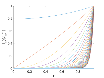
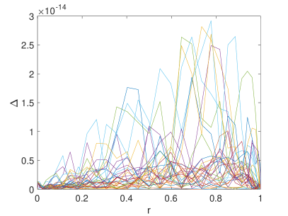
Figure 1. On the left the modified Bessel functions $I_{n}$, $n=0,1,\ldots,15$ for $r\leq 1$ normalized to 1 for $r=1$ (the higher $n$, the closer the corresponding function is to the vertical axis on the right), and the modulus of the difference between numerical and exact solution for $\psi_{1}^{(j)}$, $j=1,\ldots,N_{\phi}/2$, on the right.

The same level of accuracy is obtained for the functions $\psi^{(j)}_{2}$ for $j=1,\ldots,N_{\phi}/2$ as can be seen in Fig. 2 on the left. The corresponding errors for $j=N_{\phi}/2+1,\ldots,N_{\phi}$ are given for $\psi_{1}^{(j)}$ in the middle and $\psi_{2}^{(j)}$ on the right of Fig. 2. The errors are in all cases of the order of $10^{-14}$ or better.

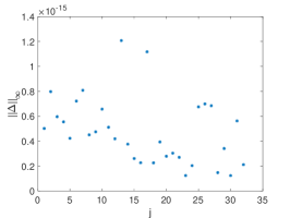
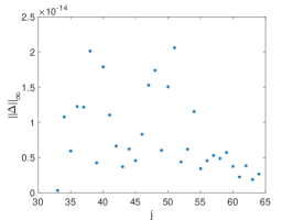
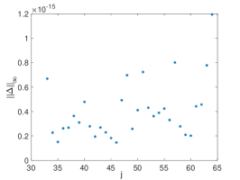
Figure 2. $L^{\infty}$ norm of the difference between numerical and exact solution for $\psi_{2}^{(j)}$, $j=1,\ldots,N_{\phi}/2$, on the left, and for $j=N_{\phi}/2+1,\ldots,N_{\phi}$ and $\psi_{1}^{(j)}$ respectively $\psi_{2}^{(j)}$ on the middle respectively on the right.

An often used, but rarely in a specific context proven result in the theory of spectral methods is that the highest spectral coefficients indicate the numerical error, see for instance [9] where it was shown that the error in the Clenshaw-Curtis integration is controlled by the highest 3 spectral coefficients (note that this can be different in the case of equations ranging over several orders of magnitude or for highly ill-conditioned problems, see for instance [10]). We test this behavior in the present context as shown in Fig. 3: on the left of the figure one can see that the maximum of the errors in Fig. 2 decreases exponentially with the number $N_{r}$ of the Chebyshev polynomials (the number of Fourier modes is always is always 64; as discussed above, due to the normalization of the solution for each Fourier mode, no decrease in the Fourier index can be expected) and the maximum of the highest Chebyshev coefficient on the right. It can be seen that the spectral coefficients are as expected a valid indicator of the numerical error and will be used in this way in the paper.

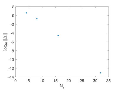
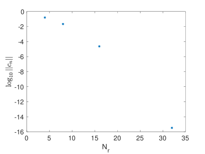
Figure 3. Maximum of the errors shown in Fig. 2 in dependence of the number of Chebyshev modes on the left, and the maximum of the highest Chebyshev coefficients for the solutions of the right.

We present the Chebyshev coefficients of the functions (31) and (32) respectively on the left respectively on the right of Fig. 4. Evidently the coefficients decrease to the order of the rounding error as expected. The apparent discontinuity at $N_{\phi}/2$ is due to the different normalization conditions for $j\leq N_{\phi}/2$ (28) and for $j>N_{\phi}/2$ (29). It is clear that increasing the number of Fourier modes $N_{\phi}$ would make it necessary to choose a larger $N_{r}$ if spatial resolution is to be maintained. Since there is only one non-trivial Fourier coefficient per function in (31) and (32), we do not consider the Fourier dependence here. In the general case, this would be, however, necessary.

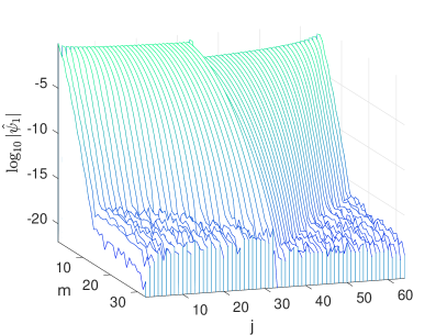
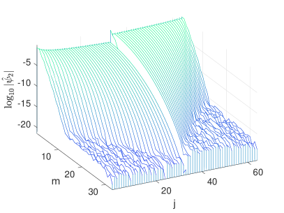
Figure 4. Modulus of the Chebyshev coefficients $\hat{\psi}_{1}^{(j)}$ (left) and $\hat{\psi}_{1}^{(j)}$ (right) of the functions given in (31) and (32).

The decrease of the coefficients with increasing Chebyshev and Fourier index is a test for the numerical approach in case there is no analytical test available. Note that the functions $\psi^{(j)}_{1,2}$ form a system of fundamental solutions and any solution can be expanded in terms of these functions. There is no decrease of the functions $\psi^{(j)}_{1,2}$ with the index $j$ though it is related to a Fourier index because of the conditions (28) and (29). However, we expect that the CGO solutions (27) built from the functions $\psi^{(j)}_{1,2}$ and satisfying the conditions (13) and (14) have spectral coefficients decreasing exponentially with Chebyshev and Fourier index as can be seen in the next section. This implies also that the $\gamma_{n}$, $n=1,\ldots,N_{\phi}$ in (27) must decrease exponentially.

4. Complex geometric optics solutions

In this section we use the fundamental solution constructed in the previous section to identify CGO solutions satisfying (28) and (29). To this end we determine the constants $\gamma_{n}$, $n=1,\ldots,N_{\phi}$ in (27) for a given $k$ via a linear system of equations. We consider the example of subsection 2.2 to illustrate the approach.

To satisfy the conditions (28) and (29), we consider the functions $\psi^{(j)}_{1,2}$ for $r=1$ in physical space, i.e., after an FFT in the variable $\phi$ for fixed $r$ for all $j=1,\ldots,N_{\phi}$. The coefficients $c_{n}$ (13) and $d_{n}$ (14) are computed for each $j$ from the products $\psi^{(j)}_{1}\exp(-k\mathrm{e}^{\mathrm{i\phi}})$ and $\psi^{(j)}_{2}\exp(k\mathrm{e}^{\mathrm{-i\phi}})$ respectively via an FFT as per (13) and (14). Because of the fast algorithm this is efficient though only the non-negative indices $n$ are needed in the first case in the conditions $c_{0}=1$ and $c_{n}=0$, $n>0$, and the non-positive indices in the conditions $d_{n}=0$, $n\leq 0$. Notice, however, that the coefficient $d_{1}$ gives the reflection coefficient via (15) which is therefore computed at the same time as the conditions on the $\gamma_{j}$.

The conditions on $c_{n}$ and $d_{n}$ lead to an $N_{\phi}$ dimensional linear system of equations for the $\gamma_{j}$, $j=1,\ldots,N_{\phi}$ in (27). For the example of Subsection 2.2, the coefficients $\gamma_{j}$, $j=1,\ldots,N_{\phi}$ can be seen in Fig. 5 on the left. As expected, the coefficients for $j\sim N_{\phi}/2$ are of the order of the rounding error (note though that $\gamma_{N_{\phi}/2+1}$ corresponds to the case $b_{0}=1$ and is thus as expected of order 1).

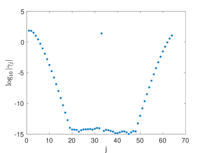
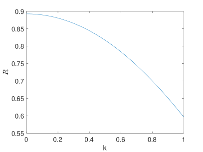
Figure 5. The coefficients $\gamma_{j}$, $j=1,\ldots,N_{\phi}$ of (27) for the example $q=1$ on the disk and $k=1$ on the left, and the reflection coefficient in dependence of $k$ on the right.

The corresponding solutions (27) can be seen in Fig. 6 on the disk. Note that the solutions are diverging for $|z|\to\infty$.

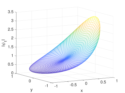
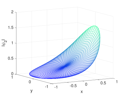
Figure 6. CGO solutions to (2) and (3) for $q=1$ on the unit disk and vanishing elsewhere for $k=1$, on the left $\psi_{1}$, on the right $\psi_{2}$.

On the other hand, the functions $\Phi_{1}$ and $\Phi_{2}$ (16) as shown in Fig. 7 are bounded for all $z\in\mathbb{C}$.

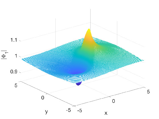
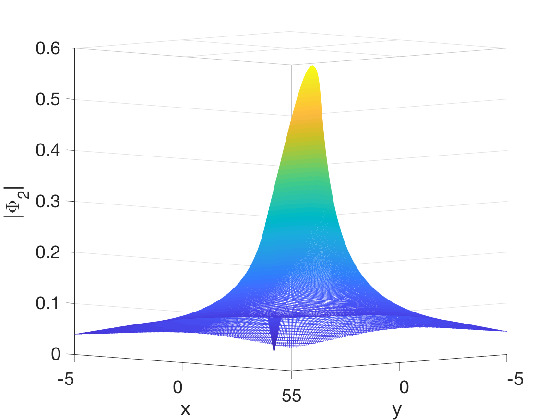
Figure 7. CGO solutions (16) to (2) and (3) for $q=1$ on the unit disk and vanishing elsewhere for $k=1$, on the left $\Phi_{1}$, on the right $\Phi_{2}$.

The spectral coefficients for the solutions to (2) and (3) are shown in Fig. 8. It can be seen that the coefficients decrease to machine precision both in the Chebyshev and in the Fourier index as already expected from the coefficients $\gamma_{j}$ in Fig. 5. This implies that the solution is resolved to the order of machine precision both in $r$ and in $\phi$.

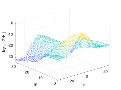
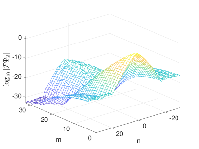
Figure 8. Spectral coefficients of the CGO solutions to (2) and (3) for $q=1$ on the unit disk and vanishing elsewhere for $k=1$, on the left for $\psi_{1}$, on the right for $\psi_{2}$.

As already mentioned, the reflection coefficient (15) is given by the scalar product of the $\gamma_{j}$ and the coefficients $d_{1}^{(j)}$ computed according to (14) for each $\psi_{2}^{(j)}$, $j=1,\ldots,N_{\phi}$ in the determination of the former. Thus it is computed at negligible cost. We show the reflection coefficient for $k\leq 1$ for the example $q=1$ on the right of Fig. 5. Note that the reflection coefficient depends only on $|k|$ because of the radial symmetry of $q(z)$, and that it is real in the studied example.

Remark 4.1.

It is of course possible to numerically implement the CGO conditions (13) and (14) for given $k$ instead of the conditions (28) and (29) in the same way as the latter. If one is only interested in the solution for one value of $k$, this is in fact more economic. In applications these solutions are in principle needed for all values of $k\in\mathbb{C}$ which means for a grid of values of $k$. The computational cost in producing the fundamental solution is $N_{\phi}$ times larger than producing the CGO solution for given $k$. Satisfying the CGO conditions for a given fundamental solution is then a lower dimensional problem since it is done for $r=1$ only. Thus as soon as one computes the CGO solutions for considerably more than $N_{\phi}$ values of $k$, the method presented in this section is clearly more economical: the main computational cost is in the determination of the fundamental solution of the last section, the CGO conditions being of lower dimension are then essentially for free.

5. Iterative solution of the d-bar system

In this section we present an iterative solution to the d-bar system (17). The same spectral approach as in the previous sections is applied to approximate the derivatives. The resulting system is solved with a Picard iteration which was shown in [28] to converge for more regular potentials for large $|k|$ like a geometric series in $1/|k|$. Here we show at concrete examples that the iteration converges very rapidly, and this for all values of $|k|$ we can access. This allows to test the codes of the previous section and the iterative approach given here by comparing their respective results. An asymptotic formula for the reflection coefficent is presented.

5.1. Fixed point iteration

The system (17) will be solved with a fixed point iteration ($j=0,1,\ldots$)

(33) $$\begin{array}[]{l}\mathrm{e}^{\mathrm{i}\phi}\left(\partial_{r}+\frac{\mathrm{i}}{r}\partial_{\phi}\right)\Phi_{1}^{(j+1)}=q(r,\phi)\mathrm{e}^{\bar{k}\bar{z}-kz}\Phi_{2}^{(j)},\\ {}\\ \mathrm{e}^{-\mathrm{i}\phi}\left(\partial_{r}-\frac{\mathrm{i}}{r}\partial_{\phi}\right)\Phi_{2}^{(j+1)}=\bar{q}(r,\phi)\mathrm{e}^{kz-\bar{k}\bar{z}}\Phi_{1}^{(j)},\end{array}$$

with the initial iterates $\Phi^{(0)}_{1}=1$ and $\Phi^{(0)}_{2}=0$.

As in the previous sections, see (22), we will apply a Chebyshev spectral method in $r$ and a discrete Fourier approach in $\phi$,

$$\begin{array}[]{l}\Phi^{(j)}_{1}\approx\sum_{\alpha=0}^{N_{r}}\sum_{\beta=-N_{\phi}/2+1}^{N_{\phi}/2}a_{\beta\alpha}^{(j)}T_{\alpha}(l)\mathrm{e}^{\mathrm{i}\beta\phi},\\ {}\\ \Phi^{(j)}_{2}\approx\sum_{\alpha=0}^{N_{r}}\sum_{\beta=-N_{\phi}/2}^{N_{\phi}/2-1}b_{\beta\alpha}^{(j)}T_{\alpha}(l)\mathrm{e}^{\mathrm{i}\beta\phi}\end{array}$$

System (33) can thus be approximated by ($m=0,1,\ldots,N_{r}$)

$$\sum_{\alpha=0}^{N_{r}}\left(D-nR\right)_{m\alpha}a_{n\alpha}^{(j+1)} =\mathbb{F}\left(q(r,\phi)\mathrm{e}^{\bar{k}\bar{z}-kz-\mathrm{i}\phi}\Phi_{2}^{(j)}\right)_{nm},\quad n=-N_{\phi}/2,\ldots,N_{\phi}/2-1,$$

(34) $$\sum_{\alpha=0}^{N_{r}}\left(D+nR\right)_{m\alpha}b_{n\alpha}^{(j+1)} =\mathbb{F}\left(\bar{q}(r,\phi)\mathrm{e}^{kz-\bar{k}\bar{z}+{\mathrm{i}\phi}}\Phi_{1}^{(j)}\right)_{nm},\quad n=-N_{\phi}/2+1,\ldots,N_{\phi}/2.$$

The matrices $D\mp nR$ are inverted by using the boundary conditions (7) which imply

$$\sum_{\alpha=0}^{N_{r}}a_{n\alpha}^{(j)}=\delta_{n0},\quad n=0,\ldots,N_{\phi}/2-1,$$

and

(35) $$\sum_{\alpha=0}^{N_{r}}b_{n\alpha}^{(j)}=0,\quad n=-N_{\phi}/2+1,\ldots,0.$$

Note that this can be seen as a simplified Newton iteration since just the diagonal part of the Jacobian

$$\mbox{Jac}=\begin{pmatrix}\bar{\partial}&-\mathrm{e}^{\bar{k}\bar{z}-kz}q/2\\ -\mathrm{e}^{kz-\bar{k}\bar{z}}\bar{q}/2&\partial\end{pmatrix}$$

(the d-bar system is linear and thus equal to $\mbox{Jac}\begin{pmatrix}\Phi_{1}\\ \Phi_{2}\end{pmatrix}=0$) is inverted with some boundary conditions.

The right-hand sides of (34) are computed in physical space to avoid convolutions. Due to the fast algorithms FFT and the FCT, this is very efficient. In the algorithm of the previous sections just one matrix $\mathcal{O}$ in (30) had to be inverted whereas here an iterative approach is used. However, the matrix $\mathcal{O}$ in (30) had to be determined via convolutions, whereas we are dealing here just with products in physical space and fast transforms.

Remark 5.1.

For each value of $n$ in (34), an $(N_{r}+1)\times(N_{r}+1)$ matrix has to be inverted which means $2N_{\phi}$ inversions of this size per iteration. The advantage with respect to the approach of the previous sections is that the system decouples here, just matrices of size $(N_{r}+1)\times(N_{r}+1)$ and $N_{\phi}\times N_{\phi}$ have to handled. This is much less demanding in terms of memory than the previous $2(N_{r}+1)N_{\phi}\times 2(N_{r}+1)N_{\phi}$ matrices in (30) (though the diagonal form of the differentiation in Fourier leads to sparse matrices there for which efficient algorithms are implemented in Matlab). Thus a much higher resolution can be reached here on the same hardware than before which is especially interesting for the case of large $|k|$. In other words, the price for the reduced memory requirements with respect to the method of the previous sections (where one big matrix had to inverted without iterating) is an iteration. The values of $N_{r}$ and $N_{\phi}$ have to be essentially chosen in a way that the factor $\mathrm{e}^{\bar{k}\bar{z}-kz}q$ is numerically resolved for given $k$ and $q$ on the disk.

The reflection coefficient $R$ (4) follows in this approach from the function $\Phi_{2}$ for $r=1$. One gets from (35)

(36) $$R=2\sum_{\alpha=0}^{N_{r}}\bar{b}_{1\alpha}.$$

5.2. Example

As in the previous sections, we consider the case of $q=1$ at the disk and vanishing outside. To test the iterative code, we compare its results for $k=1$ with the code of the previous section (recall that the fundamental solution itself was tested in section 3 by comparison with modified Bessel functions). We use $N_{r}=32$ and $N_{\phi}=64$ in both cases. The solutions $\psi_{1,2}$ are computed via the fundamental solution, the solutions $\Phi_{1,2}$ with the iterative code. The differences between the solutions $\Delta\Phi_{1}:=\mathrm{e}^{kz}\psi_{1}-\Phi_{1}$ and $\Delta\Phi_{2}:=\mathrm{e}^{\bar{k}\bar{z}}\psi_{2}-\Phi_{2}$ can be seen in Fig. 9. They are both of the order $10^{-13}$ which implies that both solutions are determined with the same precision.

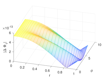
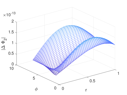
Figure 9. Differences of the CGO solutions to (2) and (3) for $q=1$ on the unit disk and vanishing elsewhere for $k=1$, obtained by the codes of the previous and the current section respectively, on the left for $\Phi_{1}$, on the right for $\Phi_{2}$.

The iteration is generally stopped when $\Delta_{\infty}:=||\Phi_{1}^{(j+1)}-\Phi_{1}^{(j)}||_{\infty}+||\Phi_{2}^{(j+1)}-\Phi_{2}^{(j)}||_{\infty}$ is smaller than $10^{-10}$. For small $|k|$, this takes roughly 30 iterations, but the iteration converges faster for larger $|k|$. We study this for three values of $k$, $k=0.1,1,10$ for the example $q=1$ on the disk. We use $N_{r}=32$ and $N_{\phi}=128$. The quantity $\Delta_{\infty}$ can be seen for these cases on the left of Fig. 10. Visibly the convergence is linear. For $k=100$, just 9 iterations are needed as can be seen on the right of Fig. 10. For the latter computation, $N_{r}=200$ and $N_{\phi}=600$ were used. Note that the convergence depends also on the norm $||q||_{\infty}$ which is here equal to 1. If much larger values are to be considered as in [2, 15], it might be necessary to solve the system (34) without iteration, i.e., as in the previous section by inverting a large matrix. We do not address this possibility here since it was not necessary for the studied examples.

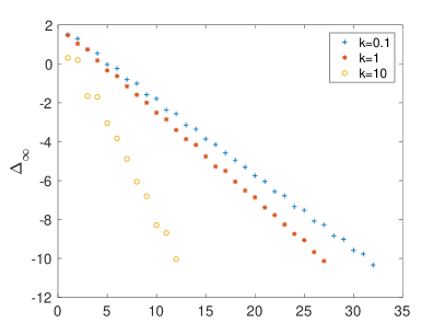
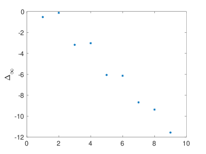
Figure 10. The quantity $\Delta_{\infty}:=||\Phi_{1}^{(j+1)}-\Phi_{1}^{(j)}||_{\infty}+||\Phi_{2}^{(j+1)}-\Phi_{2}^{(j)}||_{\infty}$ in dependence of the number of iterations $j$ for $q=1$ on the unit disk and vanishing elsewhere, on the left for $k=0.1,1,10$ and on the right for $k=100$.

The modulus of the solutions for $k=100$ can be seen in Fig. 11. The function $\Phi_{1}$ on the left of the figure appears to be roughly equal to 1 in correspondence with its asymptotic value with corrections of order $1/k$. The high frequency oscillations of the solution are hardly visible. These oscillations are much more pronounced for function $\Phi_{2}$ on the right of the same figure with amplitude of order $1/k$ around the asymptotic value 0 for the solution.

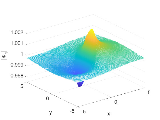
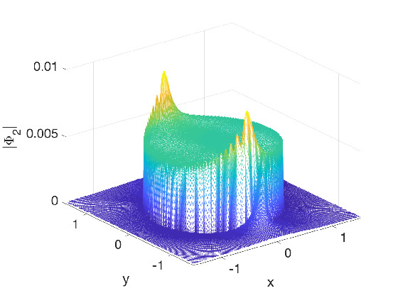
Figure 11. CGO solutions to (2) and (3) for $q=1$ on the unit disk and vanishing elsewhere for $k=100$, on the left for $\Phi_{1}$, on the right for $\Phi_{2}$.

As before, the numerical resolution can be checked via the decrease of the spectral coefficients for large value of the Chebyshev and Fourier indices. For the example $k=100$, this can be seen in Fig. 12. The coefficients decrease as expected to the order of machine precision which shows that the solutions are numerically well resolved.

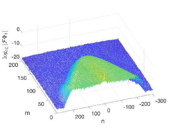
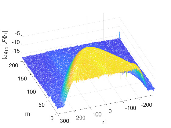
Figure 12. Spectral coefficients of CGO solutions to (2) and (3) for $q=1$ on the unit disk and vanishing elsewhere for $k=100$, on the left for $\Phi_{1}$, on the right for $\Phi_{2}$.

Note that no aliasing problems are observed here, which is due exactly to the fact that the spectral coefficients decrease both in Chebyshev and Fourier indices to machine precision. In fact much higher values of $|k|$ can be treated if this is respected. As discussed in remark 5.1, the number $N_{r}$ of Chebyshev polynomials and the number $N_{\phi}$ of Fourier modes have to be chosen such that the spectral coefficients of $q(r,\phi)\mathrm{e}^{\bar{k}\bar{z}-kz}$ decrease to machine precision. For $k=1000$ this is shown in Fig. 13 on the left. For $N_{r}=1200$ and $N_{\phi}=4400$, the spectral coefficients decrease to the order of the rounding error. With this choice of the parameter $N_{r}$ and $N_{\phi}$, the iteration converges after just 7 steps. The spectral coefficients shown in Fig. 13 decrease as expected to the order of the rounding error.

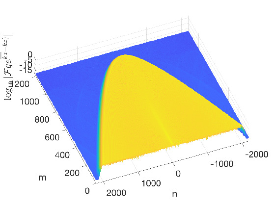
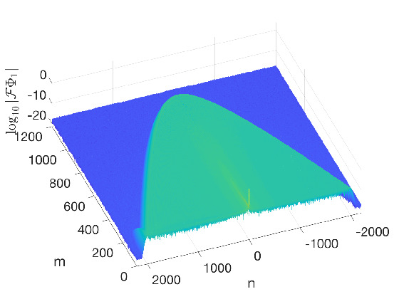
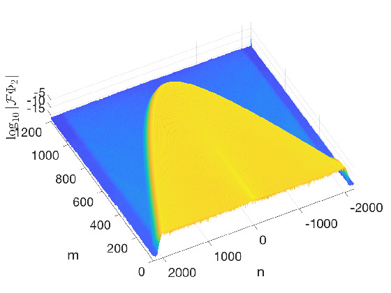
Figure 13. Spectral coefficients of $\mathrm{e}^{\bar{k}\bar{z}-kz}q$ on the left, and of CGO solutions to (2) and (3) for $q=1$ on the unit disk and vanishing elsewhere for $k=1000$, on the middle for $\Phi_{1}$, on the right for $\Phi_{2}$.

The solutions can be seen in Fig. 14. The function $\Phi_{1}$ on the left has hardly visible oscillations, the deviation from the asymptotic value 1 is of order $1/k$ as in Fig. 11. The function $\Phi_{2}$ on the right on the other hand shows rapid oscillations of order $1/k$ around 0.

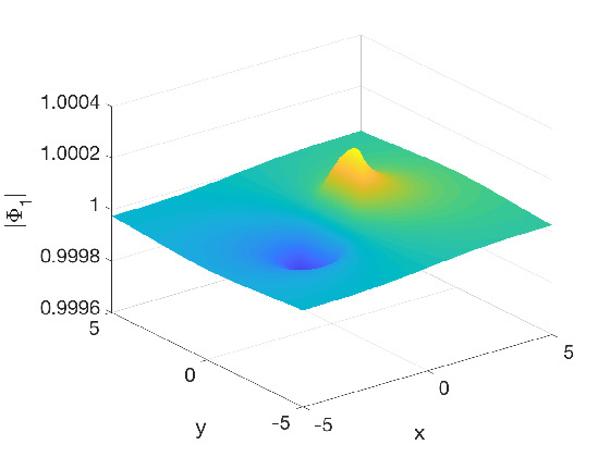
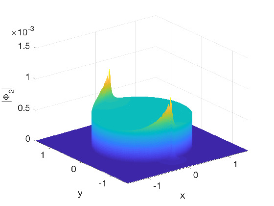
Figure 14. CGO solutions to (2) and (3) for $q=1$ on the unit disk and vanishing elsewhere for $k=1000$, on the left for $\Phi_{1}$, on the right for $\Phi_{2}$.

5.3. Reflection coefficient

The reflection coefficient can be computed for a given value of $k$ via (36). For the example of the characteristic function of the disk studied here, one gets for $k\in[1,100]$ the left figure of Fig. 15. The reflection coefficient has an amplitude decreasing proportional $1/|k|^{3/2}$ and an oscillatory singularity at infinity as can be seen from the plot of $Rk^{3/2}$ on the right of the same figure.

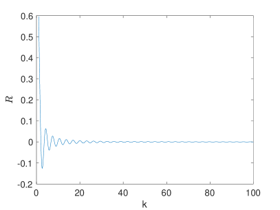
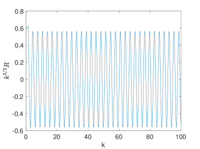
Figure 15. Reflection coefficient $R$ (4) for $q=1$ on the unit disk and vanishing elsewhere in dependence of $k$ on the left, and $kR$ on the right.

An asymptotic formula for the reflection coefficent can be obtained via (4) and (6) with $k=\kappa e^{i\psi}$, $\kappa,\psi\in\mathbb{R}$,

(37) $$\bar{R}(k)=\frac{2}{\pi}\int_{0}^{1}\int_{0}^{2\pi}q(r,\phi)e^{2i\kappa r\sin(\phi-\psi)}\Phi_{1}rdr\phi.$$

In [28] it was shown for $C^{\infty}$ potentials such that all derivatives are in $L^{2}(\mathbb{R}^{2})$ that $\Phi_{1}$ and $\Phi_{2}$ converge like a geometric series in $1/\kappa$ for $\kappa$ large. The situation is less clear for discontinuous potentials as the ones studied here, but numerical results indicate that $\Phi_{1}=1+O(1/\kappa)$ also in this case. This would imply for large $\kappa$ with a stationary phase approximation for (37) for the example of the disk (where $k$ can be chosen to be real) that

(38) $$\bar{R}(k)\approx\frac{1}{\sqrt{\pi k^{3}}}\cos(2k-3\pi/4).$$

In Fig. 16 we show on the left the numerically computed reflection coefficient in blue and in red the asymptotic formula (38). It can be seen that the agreement is excellent already for values of the order of $|k|\sim 10$. The difference between numerically computed reflection coefficient and the asymptotic formula is shown to be of the order of $k^{5/2}$ on the right.

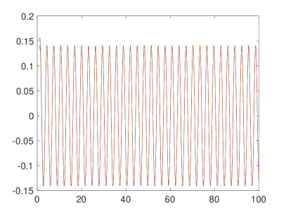
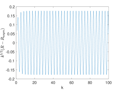
Figure 16. Reflection coefficient $R$ (4) for $q=1$ on the unit disk and vanishing elsewhere in dependence of $k$ on the left, in blue the numerical value, in red the asymptotic formula $R_{asym}$ (38), and $k^{5/2}(R-R_{asym})$ on the right.

6. Outlook

In this paper, we have presented spectral approaches for the numerical construction of CGO solutions for potentials with compact support on a disk, i.e., the scattering for the defocusing DS II equation. It is straight forward to generalize these approaches to functions which are piecewise smooth on annular parts of the disk. For large values of the modulus of the spectral parameter $|k|$, the reflection coefficient is shown to have an oscillatory behavior. An asymptotic formula is given in this case. This could allow the computation of the reflection coefficient, i.e., the scattering data for all values of $k$ with a hybrid approach: for values of $|k|\lesssim 1000$, the reflection coefficient is numerically computed to machine precision. For larger values of $|k|$, an asymptotic series in $1\sqrt{|k|}$ will be given which could also be computed for large $|k|$ to machine precision. The oscillatory nature of the reflection coefficient for $k\to\infty$ makes the use of hybrid approaches necessary in the numerical inverse scattering. This means that the main asymptotic contribution has to be treated analytically with some semiclassical techniques, and just the residual between asymptotic and full CGO solution will be computed numerically. This will be the subject of further research.

A further direction of research will be related to the exceptional points of the d-bar system (2) in the focusing case ($\sigma=-1$). The numerical tools developed in the present paper and in [15] will allow to study large classes of potentials to see in which form and when exceptional points appear, and to which physical features (appearence of lump solitons?) they correspond in the context of the focusing DS.

An interesting question in the context of potentials with compact support would be cases with a non-circular boundary. The task would be to map for instance a smooth and convex boundary with a conformal transformation to a circle. The construction of such tansformations, see for instance [14], and its combination with the codes presented here will be a direction of future research.

The present paper presents a purely spectral approach to the d-bar system (2), i.e., all functions are expanded in terms of combined Chebyshev and Fourier series which are then truncated. Actual computations are done with the coefficients of these series called spectral coefficients. Resolution in terms of Chebychev polynomials is limited by the conditioning (second order differentiation matrices are known to have a conditioning of $O(N_{r}^{4})$, see the discussion in [31]). In [26] an ultraspherical approach with better conditioning and sparser matrices was presented which was applied in the context of the hypergeometric equation in [10] to the 2d Laplace equation in polar coordinates. It was shown there that higher accuracies can be achieved than with Chebychev differentiation matrices. We will test in future publications whether this approach can also be efficient in the present context.

Note that the presented codes are highly parallelisable. First the task to compute CGO solutions for a high number of values of the spectral parameter $k$ can be done in parallel, in an efficient way on low cost GPUs as in [20]. Since the code is spectral and thus very efficient, they can be run on a single GPU for each $k$ up to rather large values of $|k|$. For exceptionally high resolutions, the codes can also be parallelised for single $k$ computation.

References

- [1] Abramowitz, M.; Stegun, I. A., eds. Handbook of mathematical functions, with formulas, graphs, and mathematical tables. National Bureau of Standards Applied Mathematics Series, 55. Dover, New York, 1965.
- [2] Assainova, O. , Klein, C. , McLaughlin, K. D. and Miller, P. D. (2019), A Study of the Direct Spectral Transform for the Defocusing Davey-Stewartson II Equation the Semiclassical Limit. Comm. Pure Appl. Math., 72: 1474-1547.
- [3] K. Astala, L. Páivárinta, J.M. Reyes, S. Siltanen, Nonlinear Fourier analysis for discontinuous conductivities: Computational results, Journal of Computational Physics 276, 74 91 (2014)
- [4] R. Beals and R. Coifman, Multidimensional inverse scattering and nonlinear PDE Proc. Symp. Pure Math. (Providence: American Mathematical Society) 43, 45-70 (1985)
- [5] R.M. Brown, Estimates for the scattering map associated with a two-dimensional first-order system. J. Nonlinear Sci. 11, no. 6, 459 471 (2001)
- [6] R. Brown and P. Perry, Soliton solutions and their (in)stability for the focusing Davey Stewartson II equation, Nonlinearity 31(9) 4290 doi.org/10.1088/1361-6544/aacc46 (2018)
- [7] R.M. Brown, G.A. Uhlmann, Communications in partial differential equations 22 (5-6), 1009-1027 (1997)
- [8] A.P. Calderón On inverse boundary value problem. Seminar on Numerical Analysis and its Applications to Continuum Physics (Rio de Janeiro, 1980) pp 65-73 (Soc. Brasil. Mat.)
- [9] C. W. Clenshaw, A. R.Curtis, A method for numerical integration on an automatic computer, Numerische Mathematik 2, 1 (1960), pp. 197-205.
- [10] S. Crespo, M. Fasondini, C. Klein, N. Stoilov, C. Vallée, Multidomain spectral method for the Gauss hypergeometric function, Numer Algor (2019). https://doi.org/10.1007/s11075-019-00741-7
- [11] T. Grava and C. Klein, Numerical study of the small dispersion limit of the Korteweg-de Vries equation and asymptotic solutions, Physica D, 10.1016/j.physd.2012.04.001 (2012).
- [12] C. Klein and K. McLaughlin, Spectral approach to D-bar problems, Comm. Pure Appl. Math., DOI: 10.1002/cpa.21684 (2017)
- [13] A. G. Gurevich, L. P. Pitaevskii, Non stationary structure of a collisionless shock waves, JEPT Letters 17 (1973), 193-195.
- [14] N. Hyvönen, L. Päivärinta, and J. P. Tamminen. Enhancing d-bar reconstructions for electrical impedance tomography with conformal maps, Inverse Problems and Imaging 12(2) (2018), 373
- [15] C. Klein, K. McLaughlin and N. Stoilov, Spectral approach to semi-classical d-bar problems with Schwartz class potentials, Physica D: Nonlinear Phenomena DOI: 10.1016/j.physd.2019.05.006 (2019)
- [16] C. Klein and K. Roidot, Numerical study of shock formation in the dispersionless Kadomtsev-Petviashvili equation and dispersive regularizations, Physica D, Vol. 265, 1-25, 10.1016/j.physd.2013.09.005 (2013).
- [17] C. Klein and K. Roidot, Numerical Study of the semiclassical limit of the Davey-Stewartson II equations, Nonlinearity 27, 2177-2214 (2014).
- [18] C. Klein, J.-C. Saut, IST versus PDE: a comparative study. Hamiltonian partial differential equations and applications, 383 449, Fields Inst. Commun., 75, Fields Inst. Res. Math. Sci., Toronto, ON, (2015)
- [19] C. Klein, C. Sparber and P. Markowich, Numerical study of oscillatory regimes in the Kadomtsev-Petviashvili equation, J. Nonl. Sci. Vol. 17(5), 429-470 (2007).
- [20] C. Klein and N. Stoilov, A numerical study of blow-up mechanisms for Davey-Stewartson II systems, Stud. Appl. Math., DOI : 10.1111/sapm.12214 (2018)
- [21] K. Knudsen, J. L. Mueller, S. Siltanen. Numerical solution method for the d-bar equation in the plane. J. Comput. Phys. 198 no. 2, 500-517 (2004).
- [22] C. Lanczos, “Trigonometric interpolation of empirical and analytic functions,” J. Math. and Phys. 17, 123–199, 1938.
- [23] P. Muller, D. Isaacson, J. Newell, and G. Saulnier. A Finite Difference Solver for the D-bar Equation. Proceedings of the 15th International Conference on Biomedical Applications of Electrical Impedance Tomography, Gananoque, Canada, 2014.
- [24] J.L. Mueller and S. Siltanen. Linear and Nonlinear Inverse Problems with Practical Applications, SIAM, 2012.
- [25] A. I. Nachman, I. Regev, and D. I. Tataru, A nonlinear Plancherel theorem with applications to global well-posedness for the defocusing Davey-Stewartson equation and to the inverse boundary value problem of Calderon, arXiv:1708.04759, 2017.
- [26] S. Olver and A. Townsend, A fast and well-conditioned spectral method, SIAM Rev. (2013), 55(3), 462 489.
- [27] P. Perry. Global well-posedness and long-time asymptotics for the defocussing Davey-Stewartson II equation in . Preprint available at arxiv.org/pdf/1110.5589v2.pdf.
- [28] J. Sjöstrand, private communication.
- [29] L.Y. Sung, An inverse scattering transform for the Davey-Stewartson equations. I, J. Math. Anal. Appl. 183 (1) (1994), 121-154.
- [30] L.Y. Sung, An inverse scattering transform for the Davey-Stewartson equations. II, J. Math. Anal. Appl. 183 (2) (1994), 289-325.
- [31] Trefethen, L.N.: Spectral Methods in Matlab. SIAM, Philadelphia (2000)
- [32] G. Uhlmann. Electrical impedance tomography and Calderón’s problem. Inverse Problems, 25(12):123011, 2009.
- [33] G. Vainikko. Multidimensional weakly singular integral equations. Lecture Notes in Mathematics 1549, Springer (1993).