Photon dispersion relations in $A_{0}$-background

Abstract

We calculate the photon dispersion relations generated by the quark loop in a quark-gluon plasma with the color $A_{0}$ background condensate $A_{0}^{c}=A_{0}^{c3}+A_{0}^{c8}$ = const. It is found that both transversal and longitudinal modes are exited. They have a gap at low momenta and are stable in high temperature approximation. The background fields act as imaginary chemical potentials and decrease the photon frequencies compared to the case of zero background. The comparison with QED plasma with chemical potential is discussed.

1 Introduction

Searching for new state of matter, quark-gluon plasma (QGP), is in the center of modern high energy physics. According to present day knowledge, it consists of quarks and gluons (or corresponding quasi-particles) deliberated from hadrons. As numerous calculations (analytic, numeric, lattice simulations, combined lattice and analytic) showed this state is not a free particle gas. The QGP background has a rather complicated structure, which is formed from a gluon field condensate, so-called $A_{0}$ condensate, and spontaneously created chromo-magnetic fields [14]. The appearance of these classical fields lowers the free energy of the plasma. This background, in particular, results in $Z(3)$ center symmetry breaking at high temperature [1]. The deconfinement phase transition order parameter is Polyakov’s loop [9]. It is the integral over temporal component of gluon field,

$$P(\vec{x})=T\exp\bigl{[}ig\int dx_{4}A_{0}(\vec{x},x_{4})\bigr{]},$$ (1)

which equals zero in confining and nonzero in deconfining phases. Various aspects of the $A_{0}$ condensation are widely discussed in the literature (see review paper [3]). The best developed part concerns the thermodynamical properties of QGP in this environment. Different models for the effective potential [12], [4], [5], [13], [10] were proposed. In particular, which is important for us here, the temperature interval where the presence of the $A_{0}$ condensate is dominant, has been estimated to be $T\sim T_{d}-2.5T_{d}$, where $T_{d}$ is deconfinement temperature [11]. At higher temperatures, the gluon quasiparticle contributions are more significant. The spectra of gluons in the $A_{0}$ background have also been calculated [7]. It was discovered, in particular, that either transversal or longitudinal modes are excited. The later ones resemble plasmons in QED plasma.

In what follows, we restrict ourselves to this interval of temperatures. Here, if necessary, the magnetic fields could be accounted for in perturbation theory.

Another important aspect of the $A_{0}$ condensate is related to the propagation and scattering processes of different particles which result in new type phenomena. These may serve as signals of the QGP creation. Scattering on the $A_{0}$ condensate as a classical external field may result in $C$-parity violating processes [2] and others.

On the other hand, Polyakov’s loop is an extended object which is not a solution to local field equations. So, the profile of the $A_{0}$ configuration is not specified and could be any, in general. In such a situation, below we consider the configuration with a constant potential, $A_{0}$ = const. It is a solution of the local field equations and can be derived from an effective two-loop potential [1], or by using other field theoretic methods (see [3]). Its relation to Polyakov’s loop is obvious. In fact, it is a good approximation for studying different processes in QGP.

In the present paper, we calculate and investigate the dispersion relations for photon in QGP in a $A_{0}$ = const background. These calculations are similar to that in [7] and fill a gap in the literature. They are also important for the phenomenology of QGP since for the detection of the plasma state we have to look for related photon modes which could exist in both the plasma and the vacuum. The quarks carry both electric and color charges and the quark loops modify the photon spectra in dependence on the color background.

The paper is organized as follows. In next section we give necessary information on quark interactions in the $A_{0}$ background and the notations used. In sect. 3 the one-loop photon polarization tensor (PT) is calculated. Sections 4 and 5 are devoted to photon dispersion relations in the high temperature approximation and for intermediate temperatures, correspondingly. Conclusions and discussion are given in the last section.
Throughout the paper we use units with $\hbar=c=k_{\rm B}=1$.

2 Lagrangian and basic formulas

We consider the color background field described by the potential $B_{\mu}^{c}=\delta_{\mu 4}(A_{0}^{c3}+A_{0}^{c8})=const$. Euclidean space-time is used. The Lagrangian describing interactions of quarks with electromagnetic and gluon fields reads

$$L=-\bar{\psi}\gamma_{\mu}V_{\mu}\psi-m\bar{\psi}\psi.$$ (2)

The matrix condensed notations are introduced. The two expressions describing electromagnetic and strong interactions are joined in (2):

$$(V_{\mu})^{ff^{\prime}}_{ij}=\left[\begin{array}[]{cc}(a_{\mu})^{ff^{\prime}}_{ij}&0\\ 0&(Q_{\mu})^{ff^{\prime}}_{ij}\end{array}\right].$$ (5)

The matrix of electromagnetic interactions has the form

$$(a_{\mu})^{ff^{\prime}}_{ij}=e~{}r_{f}A_{\mu}\delta^{ff^{\prime}}\delta^{ij},$$ (6)

and the one describing strong interactions is

$$(Q_{\mu})^{ff^{\prime}}_{ij}=gQ^{ij}_{\mu}\delta^{ff^{\prime}},$$ (7)

where the color matrix is $Q^{ij}_{\mu}=\frac{(\lambda^{a})^{ij}}{2}Q^{a}_{\mu}$ and $\lambda^{a}$ - Gell-Mann matrixes, $A_{\mu}$ and $Q_{\mu}$ denotes potential of electromagnetic and gluon field, correspondingly. In (6), (7) we marked color by Latins i, j,… = 1, 2, 3. The mass matrix is also flavor dependent: $m=m_{f}\delta_{ff^{\prime}}$. The quark wave function can be taken in the form $([\psi)^{f}_{i}]^{T}=(\psi_{i}^{u},\psi_{i}^{d},\psi_{i}^{s},...|\psi^{f}_{i=1},.\psi^{f}_{i=2},...,\psi^{f}_{i=3})$. In the expressions (6) and (7), in one matrix either the flavor or the color variables are joined. We note that a specific flavor has the corresponding electric charge. In units of proton charge we have $e_{f}=|e|r_{f}$ and the number $r_{f}$ corresponds to this flavor. For example, for $u$-quark $r_{u}=2/3$, for $d$ quark $r_{d}=-1/3$, for s-quark $r_{s}=-1/3$, etc. The electromagnetic field feels the flavor parameter $e_{r}$ of a quark whereas the gluon feels color (strong) charge $g$. In terms of these objects all the calculations can be carried out. Below we restrict ourselves to three light quarks, only.

As we see from Eq.(6), electromagnetic interaction is diagonal with respect to color and flavor variables. To account for the background color fields we take into consideration the structure of the $\lambda^{a}$ matrixes. In QCD the $A_{0}$ was calculated already by analytic methods of field theory in either gluon or quark sector (see [3]). In these cases, two background fields could be generated - $A_{0}^{3}$ and $A_{0}^{8}$, correspondingly to the diagonal generators $T^{3}=\frac{\lambda^{3}}{2}$, $T^{8}=\frac{\lambda^{8}}{2}$,

$$\lambda^{3}=\left[\begin{array}[]{ccc}1&0&0\\ 0&-1&0\\ 0&0&0\end{array}\right],~{}~{}\lambda^{8}=\frac{1}{\sqrt{3}}\left[\begin{array}[]{ccc}1&0&0\\ 0&1&0\\ 0&0&-2\end{array}\right].$$ (14)

The background fields $B^{c}_{\mu}=\delta_{\mu 0}(\delta^{c3}A^{3}_{0}+\delta^{c8}A^{8}_{0})$ belong to the gauge group center:

$$A_{0}=\frac{2\pi n}{g\beta},~{}~{}n\to Z_{3}:$$ (15)

$\beta=1/T$, T is temperature.

In [15] - [16] it was obtained that in two-loop approximation the condensed fields are:

$$gA_{0}^{3}=\frac{g^{2}T}{4\pi}(3-\xi),~{}~{}A_{0}^{8}=0.$$ (16)

$\xi$ is gauge fixing parameter.

We have to expect that $A_{0}^{8}\not=0$ in general. It can happen in higher orders in loop expansion. It is also important that the value of the created field does not depend on the quark mass.

For our problem with photon PT, the actual values of the background fields are not very essential and so we consider two scenarios: 1) The situation happening in the case of (16); 2) the case $B_{0}^{3},B_{0}^{8}\not=0$.

Since the latter case is more general, we continue for this one. Let us take into account the light quark flavors: $f=u(m_{u},e_{u}=2/3e),~{}d(m_{d},e_{d}=-1/3e),~{}s(m_{s},e_{s}=-1/3e)$. $e$ is proton electric charge. Accounting for the matrix structure of the generators $T^{3},T^{8}$ (14), we have to put the background fields for quark flavors: $B_{0}^{u}=(+A_{0}^{3}+A_{0}^{8}/\sqrt{3})/2,2/3e,m_{u}$ for u-quark; $B_{0}^{d}=(-A_{0}^{3}+A_{0}^{8}/\sqrt{3})/2,-1/3e,m_{d}$ for d-quark and $B_{0}^{s}=-A_{0}^{8}/\sqrt{3},e_{s}=-1/3e,m_{s}$  for s-quark. These have to be multiplied by the coupling g in the covariant derivatives.

Now, we turn to calculation of one-loop photon PT at these background at high temperature $T>T_{d}$. Standard imaginary time formalism is used. In this formulation, the fermion propagator at $A_{0}$ background has a fourth momentum component $p_{4}=2\pi Tl-A_{0}$ with half-integer $l$. In what follows the notations will be used: $p_{\mu}=(p_{4},\mathbf{p})_{\mu}$ and $\underline{p}$ is $p_{\mu}$ written without index, $\mathbf{p}$ is spatial part and $p=|\mathbf{p}|$. The same conventions are used for $k$.

3 Photon polarization tensor

We start from the Schwinger-Dyson equation for the photon propagator (PT),

$${\mathscr{D}}^{-1}_{\mu\nu} ={\mathscr{D}^{(0)}}^{-1}_{\mu\nu}-\Pi_{\mu\nu}(\underline{k})$$ (17)

where ${\mathscr{D}^{(0)}}^{-1}_{\mu\nu}$ is inverse free field propagator. The photon PT accounting for a one flavor is given by

$$\Pi^{\rm G}(\underline{k})_{\mu\nu} =-e^{2}T\sum_{l=-\infty}^{\infty}\int\frac{d^{3}p}{(2\pi)^{3}}{\rm Tr}\,\gamma_{\mu}\frac{1}{\not{p}-m}\gamma_{\nu}\frac{1}{\not{p}-\not{k}-m},$$ (18)

$$=e^{2}T\sum_{l=-\infty}^{\infty}\int\frac{d^{3}p}{(2\pi)^{3}}\frac{Z_{\mu\nu}}{(p^{2}+m^{2})((p-k)^{2}+m^{2})},$$

where the minus sign is from the Fermion loop and $e=e_{f}$ is the electric charge. In the following we drop the index ’$f$’ and the sum over ’$f$’. In the second line we defined

$$Z_{\lambda\lambda^{\prime}} =-{\rm Tr}\gamma_{\mu}(\not{p}+m)\gamma_{\nu}(\not{p}-\not{k}+m)$$ (19)

for the polynomial in the numerator. Carrying out the trace (it is Euclidean) we get

$$\frac{1}{4}Z_{\mu\nu} =\delta_{\lambda\lambda^{\prime}}(\underline{p}(\underline{p}-\underline{k})+m^{2})-p_{\lambda}(p-k)_{\lambda^{\prime}}-(p-k)_{\lambda}p_{\lambda^{\prime}}.$$ (20)

Below we need the combinations

$$\frac{1}{4}Z_{44} =-p_{4}(p-k)_{4}+\mathbf{p}(\mathbf{p}-\mathbf{k})+m^{2},$$ (21)

$$\frac{1}{4}Z_{\mu\mu} =2\underline{p}(\underline{p}-\underline{k})+4m^{2}.$$

We divide the expression (17) for the polarization tensor into vacuum and temperature parts,

$$\Pi_{\mu\nu}(\underline{k}) =\Pi^{\rm vac.}_{\mu\nu}(\underline{k})+\Delta_{T}\Pi_{\mu\nu}(\underline{k}).$$ (22)

The vacuum part has the simple tensor structure

$$\Pi^{\rm vac.}_{\mu\nu}(\underline{k}) =\left(\delta_{\mu\nu}{\underline{k}^{2}}-{k_{\mu}k_{\nu}}\right)\Pi(\underline{k}^{2})$$ (23)

and the representation in terms of a parametric integration of $\Pi(\underline{k}^{2})$ is

$$\Pi(\underline{k}^{2}) =-\frac{e^{2}}{8\pi^{2}}\int_{0}^{1}dx\,x(1-x)\ln\left(1-x(1-x)\frac{\underline{k}^{2}}{m^{2}}\right).$$ (24)

In the temperature dependent part we use the following formula. Let

$$\Pi_{\mu\nu}(\underline{k}) =Te^{2}\sum_{l=-\infty}^{\infty}\int\frac{d^{3}p}{(2\pi)^{3}}\frac{Z(p_{4},\mathbf{p})_{\mu\nu}}{(p^{2}+m^{2})((p-k)^{2}+m^{2})}$$ (25)

be the analytic expression for a one-loop graph with two lines and $Z(p_{4},\mathbf{p})_{\mu\nu}$ be the polynomial in the numerator, where we explicitly indicated its dependence on the integration momenta. Then

$$\Delta_{T}\Pi_{\mu\nu}(\underline{k}) =e^{2}\int\frac{d^{3}p}{(2\pi)^{3}}\frac{1}{2{E_{p}}}\left\{n_{s}\left[\frac{Z_{\mu\nu}(i{E_{p}},\mathbf{p})+Z_{\mu\nu}(-i{E_{p}}-k_{4},-\mathbf{p}-\mathbf{k})}{N}+{\rm c.c.}\right]\right.$$ (26)

$$\left.~{}~{}~{}~{}~{}~{}~{}~{}~{}~{}~{}~{}~{}~{}~{}~{}~{}~{}~{}~{}~{}~{}~{}~{}~{}~{}~{}~{}~{}~{}~{}~{}~{}~{}~{}~{}~{}~{}~{}~{}~{}+n_{a}\left[\frac{Z_{\mu\nu}(i{E_{p}},\mathbf{p})-Z_{\mu\nu}(-i{E_{p}}-k_{4},-\mathbf{p}-\mathbf{k})}{N}-{\rm c.c.}\right]\right\},$$

with

$${E_{p}}=\sqrt{p^{2}+m^{2}},\ \ N=\underline{k}^{2}+2ik_{4}{E_{p}}+2\mathbf{p}\mathbf{k},$$ (27)

and

$$n_{s}=\frac{1}{2}(n_{A_{0}}+n_{-A_{0}}),\ \ n_{a}=\frac{1}{2}(n_{A_{0}}-n_{-A_{0}}),\ \ n_{A_{0}}=\frac{-1}{\exp(\beta({E_{p}}+iA_{0}))+1}$$ (28)

is the combination with the Boltzmann factor for fermions. The notation $+c.c.$ prescribes to add the complex conjugated of the term given in the bracket. The background field $A_{0}$ appears only in the Boltzmann factors. In the following, the antisymmetric combinations, i.e., the second term in the square bracket in (26), will disappear after taking the angular integrations. We mention that these formulas are formally the same as for the QED in a dense medium with the substitution $\mu\to iA_{0}$ for the chemical potential. In case of $A_{0}$-condensate, however, $\Delta_{T}\Pi_{\mu\nu}(\underline{k})$ is a periodic function of $A_{0}$ with period $2\pi T$.

Applying (26) to our expressions (21) we note the substitutions

$$\frac{1}{4}Z_{44} \to N-4ik_{4}{E_{p}}+4{E_{p}}^{2}-\underline{k}^{2},$$ (29)

$$\frac{1}{4}Z_{\mu\mu} \to 2(N-\underline{k}^{2}+2m^{2}).$$

and get from (18) and (21)

$$\Delta_{T}\Pi_{44} =4e^{2}\int\frac{d^{3}p}{(2\pi)^{3}}\frac{n_{s}}{2{E_{p}}}\left(1-\frac{\underline{k}^{2}-4{E_{p}}^{2}+4ik_{4}{E_{p}}}{N}+{\rm c.c.}\right),$$ (30)

$$\Delta_{T}\Pi_{\mu\mu} =4e^{2}\int\frac{d^{3}p}{(2\pi)^{3}}\frac{n_{s}}{2{E_{p}}}2\left(1-\frac{\underline{k}^{2}-2m^{2}}{N}+{\rm c.c.}\right).$$

In these formulas the angular integration can be carried out using known formulas (see, e.g., [6])

$$\int_{0}^{\pi}d\theta\sin(\theta)\frac{1}{N}=\frac{\ln(a)-\ln(b)}{4pk}$$ (31)

with the angle $\theta$ between the vectors $\mathbf{p}$ and $\mathbf{k}$ such that $\mathbf{p}\mathbf{k}=pk\cos(\theta)$ holds and the notations

$$\ln a =\frac{(\underline{k}^{2}+2pk)^{2}+4k_{4}^{2}{E_{p}}^{2}}{(\underline{k}^{2}-2pk)^{2}+4k_{4}^{2}{E_{p}}^{2}},\ \ \ln b=\ln\frac{\underline{k}^{4}-4(pk-ik_{4}{E_{p}})^{2}}{\underline{k}^{4}-4(pk+ik_{4}{E_{p}})^{2}}$$ (32)

were introduced. We mention that the above expressions were initially defined for real $k_{4}$ and allow for direct continuation to real frequencies, $k_{4}\to-i\omega$.

Using with (27) the relation

$$2\mathbf{p}\mathbf{k}=N-\underline{k}^{2}-2ik_{4}{E_{p}},$$ (33)

after angular integration by means of (31) the expressions (30) turn into

$$\Delta_{T}\Pi_{44}(k) =\frac{2}{\pi^{2}}e^{2}\int_{0}^{\infty}\frac{dp\,p^{2}}{{E_{p}}}\,n_{s}M_{44},$$

$$\Delta_{T}\Pi_{\mu\mu}(k) =\frac{2}{\pi^{2}}e^{2}\int_{0}^{\infty}\frac{dp\,p^{2}}{{E_{p}}}\,n_{s}M_{\mu\mu},$$

$$\Delta_{T}A(k) =\frac{2}{\pi^{2}}e^{2}\int_{0}^{\infty}\frac{dp\,p^{2}}{{E_{p}}}\,n_{s}M_{A},$$ (34)

with

$$M_{44} =1-\frac{(\underline{k}^{2}-4{E_{p}}^{2})\ln(a)-4ik_{4}{E_{p}}\ln(b)}{8pk},$$

$$M_{\mu\mu} =1-\frac{(\underline{k}^{2}-2m^{2})\ln(a)}{8pk},$$

$$M_{A} =1-\frac{k_{4}^{2}}{k^{2}}+\frac{(k_{4}^{4}-k^{4}-4p^{2}\underline{k}^{2}-4{E_{p}}^{2}k_{4}^{2})\ln(a)-4ik_{4}{E_{p}}\underline{k}^{2}\ln(b)}{8pk^{3}},$$ (35)

where we also displayed the expressions for the combination $A=\frac{1}{2}\Pi_{\mu\mu}-\frac{\underline{k}^{2}}{2\mathbf{k}^{2}}\Pi_{44}$, which will appear below for the transversal mode.

Further we have to consider the tensor structures. We use the following notations,

$$A_{\mu\nu} =\delta_{\mu\nu}-\frac{k_{\mu}k_{\nu}}{\underline{k}^{2}}-h_{\mu}h_{\nu},\ \ B_{\mu\nu}=h_{\mu}h_{\nu},\ \ h_{\mu}=\frac{k_{4}}{k\underline{k}}k_{\mu}-\frac{\underline{k}}{k}u_{\mu},\ \ u_{\mu}=\delta_{\mu 4}$$ (36)

for the two independent tensor structures which we have at finite temperature. The polarization tensor has the decomposition

$$\Pi_{\mu\nu}=A_{\mu\nu}\Pi_{t}+B_{\mu\nu}\Pi_{l}$$ (37)

with

$$\Pi_{l} =\frac{\underline{k}^{2}}{k^{2}}\Pi_{44},\ \ \Pi_{t}\equiv A=\frac{1}{2}\Pi_{\mu\mu}-\frac{\underline{k}^{2}}{2k^{2}}\Pi_{44}.$$ (38)

With these notations and the free inverse photon propagator,

$${\mathscr{D}^{(0)}}^{-1}_{\mu\nu}=(\delta_{\mu\nu}\underline{k}^{2}-k_{\mu}k_{\nu}),$$ (39)

one has the (also well known) formula

$$\mathscr{D}_{\mu\nu} =\frac{1}{\underline{k}^{2}-A}A_{\mu\nu}+\frac{k^{2}/\underline{k}^{2}}{k^{2}-\Pi_{44}}B_{\mu\nu}$$ (40)

whose poles determine the spectrum. The excitations which go with $A_{\mu\nu}$ are transversal (there are two of them with equal spectrum) and that going with $B_{\mu\nu}$ are longitudinal.

Splitting the vacuum part of the polarization tensor according to (37), we get from (23) and (36)

$$\Pi^{\rm vac.}_{\mu\nu}(\underline{k}) =(A_{\mu\nu}+B_{\mu\nu})\underline{k}^{2}\Pi(\underline{k}^{2})$$ (41)

and together with (38) we arrive at

$$A =\underline{k}^{2}\Pi(\underline{k}^{2})+\Delta_{T}A,\ \ \Pi_{44}=k^{2}\Pi(\underline{k}^{2})+\Delta_{T}\Pi_{44}.$$ (42)

Finally, from (40) the dispersion equations

$$\underline{k} =\underline{k}^{2}\Pi(\underline{k}^{2})+\Delta_{T}A,\ \ \ k^{2}=k^{2}\Pi(\underline{k}^{2})+\Delta_{T}\Pi_{44}$$ (43)

follow.

4 Spectra at high temperature

In this section we consider the spectrum in leading order for $T\to\infty$. In this case expressions significantly simplify. First of all, since the temperature dependent part of the polarization tensor is of order $T^{2}$ (see below), the vacuum part is subleading. In the temperature dependent part, the leading order comes from the expansions of $M_{44}$ and $M_{A}$, (32), for $\mathbf{p}\to\infty$,

$$M_{44} =M_{44}^{\rm lead.}+\dots\,,\ \ \mbox{with}\ M_{44}^{\rm lead.}=2+\frac{\omega}{k}\ln\frac{\omega-k}{\omega+k},$$

$$M_{A} =M_{A}^{\rm lead.}+\dots\,,\ \ \mbox{with}\ M_{A}^{\rm lead.}=\frac{\omega^{2}}{k^{2}}-\frac{1}{2}\left(1-\frac{\omega^{2}}{k^{2}}\right)\frac{\omega}{k}\ln\frac{\omega-k}{\omega+k},$$ (44)

which can be also represented using the function (eq. (2.2.3) in [6])

$$F(x) =-\frac{x}{2}\left(\ln\left|\frac{x-1}{x+1}\right|+i\pi\Theta(1-x)\right)$$ (45)

as

$$M_{44}^{\rm lead.} =2\left(1-F\left(\frac{\omega}{k}\right)\right),$$

$$M_{A}^{\rm lead.} =\left(\frac{\omega}{k}\right)^{2}+\left(1-\left(\frac{\omega}{k}\right)^{2}\right)F\left(\frac{\omega}{k}\right).$$ (46)

The last formulas give at once the analytic continuation to $\omega>k$.

After this expansion, the integrals over $p$ in (31) can be carried out and we arrive at

$$\Delta_{T}\Pi_{44}(k) =\Lambda^{2}M_{44}^{\rm lead.}+\dots\,,$$

$$\Delta_{T}A(k) =\Lambda^{2}M_{A}^{\rm lead.}+\dots\,,$$ (47)

where we defined

$$\Lambda^{2} =-\frac{2e^{2}}{\pi^{2}}\int_{0}^{\infty}\frac{dp\,p^{2}}{{E_{p}}}\,n_{s}=\frac{2e^{2}}{\pi^{2}}\left(\frac{\pi^{2}T^{2}}{12}-\frac{m^{2}+A_{0}^{2}}{4}\right)=e^{2}\left(\frac{T^{2}}{6}-\frac{m^{2}+A_{0}^{2}}{2\pi^{2}}\right),$$ (48)

which is the remaining integration over $p$ and involved the Boltzmann factors defined in (28). In the right side is the expansion for large $T$ assuming $m$ and $A_{0}$ are of order $T$. In case $m=0$ and arbitrary $A_{0}$ we get for large $T$

$$\Lambda^{2} =\frac{T^{2}}{\pi^{2}}\left(-{\rm Li}_{2}\left(-e^{iA_{0}/T}\right)-{\rm Li}_{2}\left(-e^{-iA_{0}/T}\right)\right),$$ (49)

which is a periodic function of $A_{0}$ and takes also negative values.

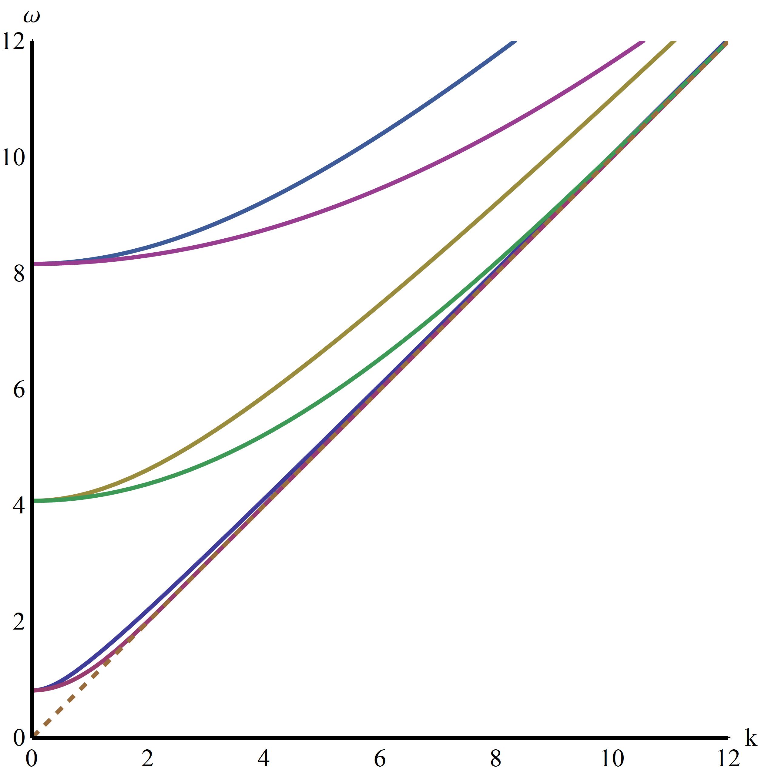
Figure 1: Solutions $\omega_{T}(k)$ (upper curve in each pair) and $\omega_{L}(k)$ (lower curve in each pair) of the dispersion relations (43) for high temperature as function of $k$ for $\Lambda=10,\ 5,\ 1$ (from top to bottom). All solutions approach $\omega=k$ for $k\to\infty$ (dashed line) and start in $\omega_{T,L}(0)=\sqrt{\frac{2}{3}}\Lambda$ (see Eq. (4)).

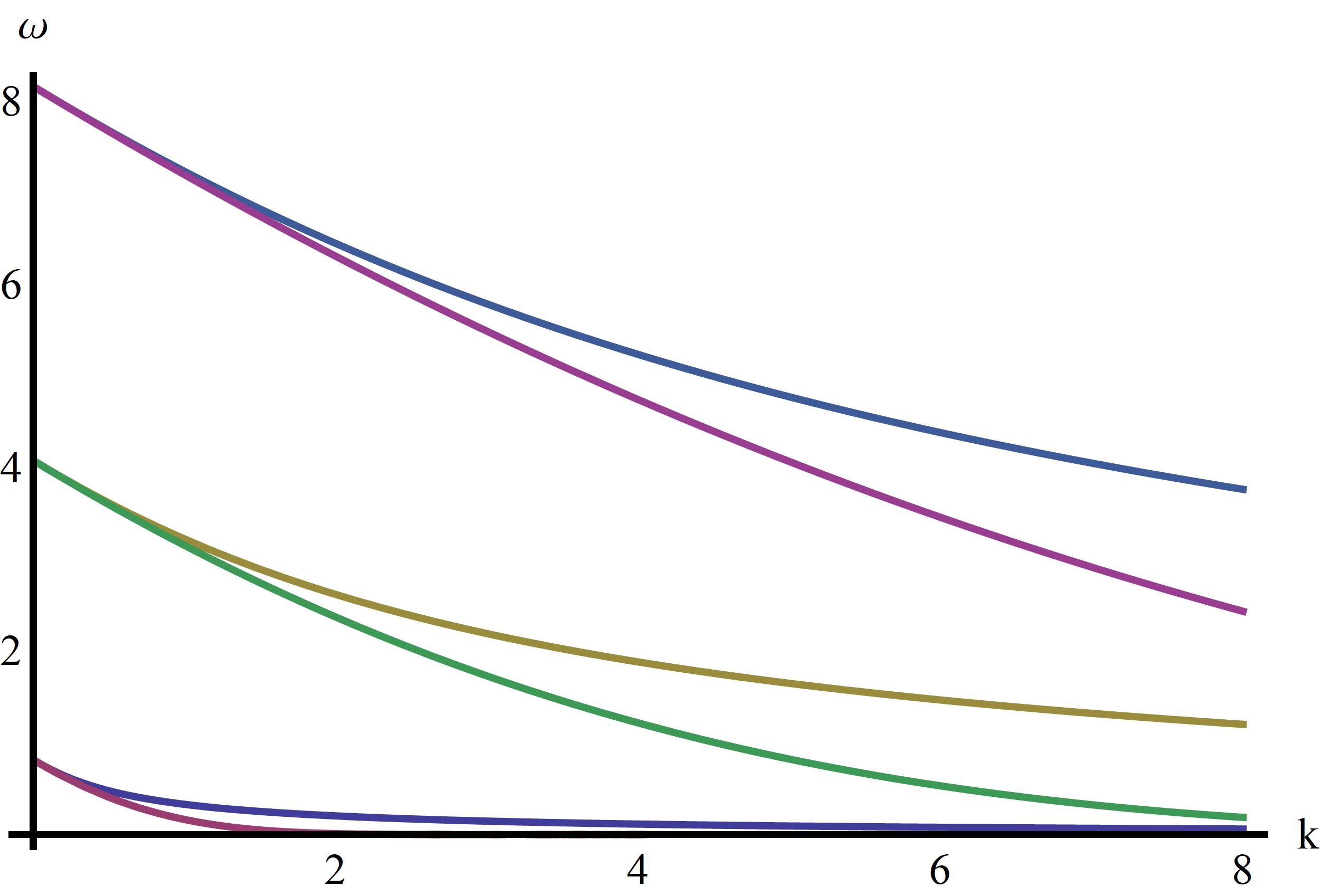
Figure 2: Deviation of the solutions of the dispersion relations (43) from momentum $k$, $\omega_{T}(k)-k$ (upper curve in each pair) and $\omega_{L}(k)-k$ (lower curve in each pair) as function of $k$ for $\Lambda=10,\ 5,\ 1$ (from top to bottom).

Turning in the dispersion equations (43) to real frequency we get for $T\to\infty$ the equations

$$\omega^{2} =k^{2}+\Lambda^{2}\left(\frac{\omega^{2}}{k^{2}}-\frac{1}{2}\left(1-\frac{\omega^{2}}{k^{2}}\right)\frac{\omega}{k}\ln\frac{\omega-k}{\omega+k}\right),$$

$$k^{2} =-\Lambda^{2}\left(2+\frac{\omega^{2}}{k^{2}}\ln\frac{\omega-k}{\omega+k}\right).$$ (50)

These equations have a scale invariance. We define

$$\omega=\Lambda\tilde{\omega},\ \ \ {k}=\Lambda\tilde{k}$$ (51)

and the equations turn into

$$\tilde{\omega}^{2} =\tilde{k}^{2}-\left(\frac{\tilde{\omega}^{2}}{\tilde{k}^{2}}-\frac{1}{2}\left(1-\frac{\tilde{\omega}^{2}}{\tilde{k}^{2}}\right)\frac{\tilde{\omega}}{\tilde{k}}\ln\frac{\tilde{\omega}-\tilde{k}}{\tilde{\omega}+\tilde{k}}\right)$$

$$\tilde{k}^{2} {=-\left(2+\frac{\tilde{\omega}^{2}}{\tilde{k}^{2}}\ln\frac{\tilde{\omega}-\tilde{k}}{\tilde{\omega}+\tilde{k}}\right)}.$$ (52)

We denote the solutions of these two equations by $\tilde{\omega}_{T}(\tilde{k})$ and $\tilde{\omega}_{L}(\tilde{k})$. Their expansions for small $k$ can be obtained by iteration and read

$$\tilde{\omega}_{T}(\tilde{k}) =\sqrt{\frac{2}{3}}\left(1+\frac{9}{10}\tilde{k}^{2}+\dots\right),$$

$$\tilde{\omega}_{L}(\tilde{k}) =\sqrt{\frac{2}{3}}\left(1+\frac{3}{10}\tilde{k}^{2}+\dots\right).$$ (53)

The behavior for large $\tilde{k}$ is

$$\tilde{\omega}_{T}(\tilde{k}) =\tilde{k}\left(1+\frac{1}{\tilde{k}^{2}}+\dots\right),$$

$$\tilde{\omega}_{L}(\tilde{k}) =\tilde{k}\left(1+2e^{-\tilde{k}-2}+\dots\right).$$ (54)

The inequality $\tilde{k}<\tilde{\omega}_{L}<\tilde{\omega}_{T}$ holds. It must be mentioned that the expansions for $k\to\infty$ are valid for the solutions of the equations (4), but not for the equations (43) since in this section we assume $T$ to be the largest quantity. We mention that up to notations these formulas are in agreement with those in [8], which were derived for QED in a dense medium.

Restoring the dependence on $\Lambda$ using (48) and denoting the solutions of (4) by $\omega_{{T},{L}}(k)$ we arrive at

$$\omega_{T}(k) =\Lambda\tilde{\omega}_{T}\left(\frac{k}{\Lambda}\right),\ \ \omega_{L}(k)=\Lambda\tilde{\omega}_{L}\left(\frac{k}{\Lambda}\right).$$ (55)

These functions are shown in Fig. 1 for several values of $\Lambda$, (48). As can be seen, the condensate $A_{0}$ lowers the photon frequency. The gap in both spectra is $\frac{2}{3}\Lambda$. In the given high-$T$ approximation both spectra are stable (an imaginary part appears only in next-to-leading order). Fig. 2 shows the deviations of the solutions from the line $\omega=k$.

5 Imaginary part at high temperature

As seen from the solution shown in Fig. 1 and from the equations (4), there is no imaginary part to order $T^{2}$. Thus we consider the next order, i.e., the order $T$, where an imaginary part may appear. We put $m=0$ for simplifying expressions. In order to derive these we return to eqs. (3) and consider the continuation $k_{4}\to-i(\omega+i0)$. We represent (3) in the form

$$M_{44} =1+M_{44}^{a}\ln(a)+M_{44}^{b}\ln(b),$$

$$M_{A} =1+\frac{\omega^{2}}{k^{2}}+M_{A}^{a}\ln(a)+M_{A}^{b}\ln(b),$$ (56)

where

$$M_{44}^{a} =\frac{1}{8pk}\left(\omega^{2}-k^{2}+4{E_{p}}^{2}\right),\ \ \ M_{44}^{b}=\frac{\omega{E_{p}}}{2pk}$$

$$M_{A}^{a} =\frac{1}{8pk^{3}}\left(-\omega^{4}-k^{4}-4p^{2}(-\omega^{2}+k^{2})+4\omega^{2}{E_{p}}^{2}\right),\ \ \ M_{A}^{b}=\frac{\omega(\omega^{2}-k^{2}){E_{p}}}{2pk^{3}}.$$ (57)

Further we need the imaginary parts of $\ln(a)$ and $\ln(b)$. For that we return to (32) and represent

$$\ln(a) =\ln\left(\frac{(2p-(\omega-k))(2p-(-\omega-k))}{(2p-(\omega+k))(2p-(-\omega+k))}\right),$$

$$\ln(b) =2\ln\left(\frac{\omega-k}{\omega+k}\right)+\ln\left(\frac{(2p-(\omega+k))(2p-(-\omega-k))}{(2p-(\omega-k))(2p-(-\omega+k))}\right).$$ (58)

Starting point for the analytic continuation in (5) is eq. (31), where for $p\to\infty$ and $\omega>k$ we have $\ln(a)\simeq 0$ and $\ln(b)\simeq 2\ln\left(\frac{\omega-k}{\omega+k}\right)$ which is real. Starting from here, the continuation is done with $\Im(\omega)>0$ and results in,
for $\omega<k$,

$$\Im(\ln(a)) =i\pi\Theta(-\omega+k<2p<\omega+k),\ \ \Im(\ln(b))=i\pi\Theta(\omega+k<2p),$$ (59)

and for $\omega>k$,

$$\Im(\ln(a)) =i\pi\Theta(\omega-k<2p<\omega+k),\ \ \Im(\ln(b))=-i\pi\Theta(\omega-k<2p<\omega+k).$$ (60)

We insert these and (5) into (3) and get for the imaginary parts,
for $\omega<k$,

$$\Im(\Pi_{44}) =\frac{1}{\pi}\int_{-\omega+k}^{\omega+k}\frac{dp\,p^{2}}{{E_{p}}}n_{s}M_{44}^{a}+\frac{1}{\pi}\int_{\omega+k}^{\infty}\frac{dp\,p^{2}}{{E_{p}}}n_{s}M_{44}^{b},$$

$$\Im(\Pi_{A}) =\frac{1}{\pi}\int_{-\omega+k}^{\omega+k}\frac{dp\,p^{2}}{{E_{p}}}n_{s}M_{A}^{a}+\frac{1}{\pi}\int_{\omega+k}^{\infty}\frac{dp\,p^{2}}{{E_{p}}}n_{s}M_{44}^{b},$$ (61)

and for $\omega>k$,

$$\Im(\Pi_{44}) =\frac{1}{\pi}\int_{-\omega+k}^{\omega+k}\frac{dp\,p^{2}}{{E_{p}}}n_{s}\left(M_{44}^{a}-M_{44}^{b}\right),$$

$$\Im(\Pi_{A}) =\frac{1}{\pi}\int_{-\omega+k}^{\omega+k}\frac{dp\,p^{2}}{{E_{p}}}n_{s}\left(M_{A}^{a}-M_{44}^{b}\right).$$ (62)

These expressions behave very differently for the regions with frequency above $k$ and below. First we discuss the behavior for $\omega>k$, which is the region where we found the solutions shown in Fig. 1. To calculate the imaginary parts for high temperature we expand the function $n_{s}$, (28),

$$n_{s}=\frac{T}{{E_{p}}^{2}+A_{0}^{2}}+O(1).$$ (63)

This expansion can be inserted into (5) since the integration region is finite. From (5) we get

$$\Im(\Pi_{44}) =\frac{T}{\pi}\int_{-\omega+k}^{\omega+k}\frac{dp\,p^{2}}{{E_{p}}({E_{p}}+A_{0}^{2})}\left(M_{44}^{a}-M_{44}^{b}\right),$$

$$\Im(\Pi_{A}) =\frac{T}{\pi}\int_{-\omega+k}^{\omega+k}\frac{dp\,p^{2}}{{E_{p}}({E_{p}}+A_{0}^{2})}\left(M_{A}^{a}-M_{44}^{b}\right).$$ (64)

These formulas demonstrate that the imaginary part on the solutions (55) is of order $T$, i.e., is of subleading order.

As concerns the region with $\omega<k$, as seen from eq. (5), we have contributions where the integration over $p$ goes up to infinity. Here we cannot use the expansion (63). Instead we have to do the substitution $p\to Tp$ and must expand the factors in the parenthesis in the integrand for large argument in the same manner as we did in section 4. As a result we get contributions of order $T^{2}$, which is in agreement with the imaginary part which we would get in (4) for $\omega>k$ (see Eq. (45)). However, this is not the region where we have the solutions of the dispersion relations and thus this region is not physical.

6 Spectra at finite temperature

In this section we discuss some topics related to the spectra at finite temperature. This means, we do not make the approximation resulting in (4). First of all we have to consider the vacuum contribution (23). We rewrite the first equation (43) with $k_{4}=-i\omega$,

$$\omega^{2}(1-\Pi(\underline{k}^{2})) =k^{2}(1-\Pi(\underline{k}^{2}))+\Delta_{T}A.$$ (65)

Figure 3: Real and imaginary parts of the vacuum contribution (65) to the polarization tensor for $m=1$, $e=1$.

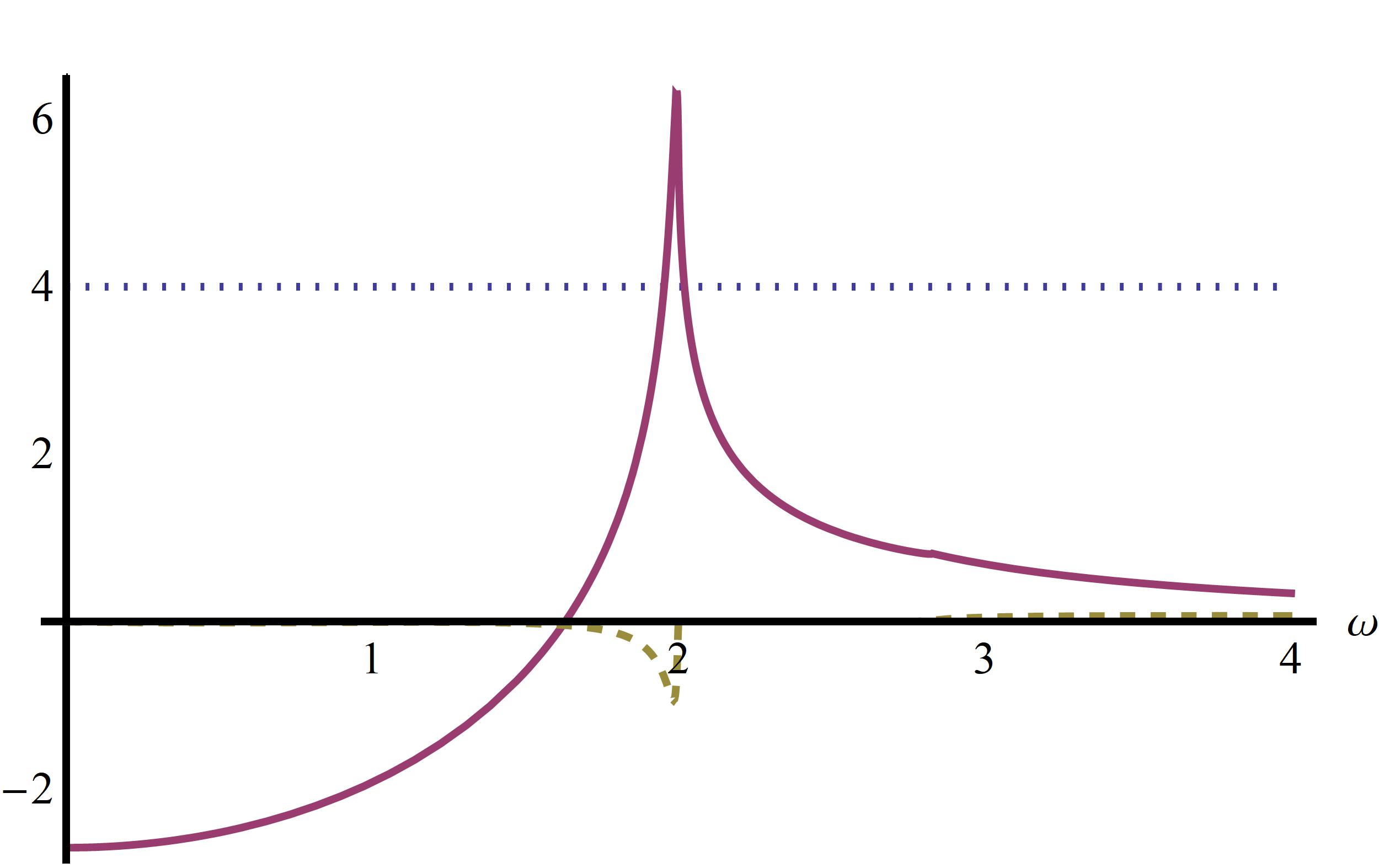
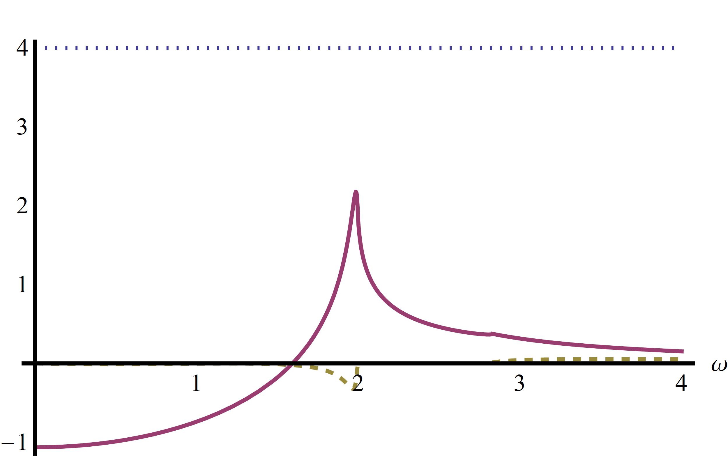
Figure 4: Left side (dotted line) and right side (solid line for real part, dashed line for imaginary part) of equation (65) for the longitudinal dispersion relation for $m=1$, $e=1$. The temperature is $T=3$ in the left panel and $T=2$ in the right panel.

The function $\Pi(\underline{k}^{2})$ can be easily plotted, see Fig. 3. It is seen that it is a quite small quantity (unless the coupling is extremely large). For large $k$ it has the behavior $\Pi\sim-\frac{1}{24\pi^{2}}\ln(k)$, thus $1-\Pi(\underline{k}^{2})$ does not change sign and we can divide by this factor. In general, it is useful to remember that without temperature contributions, the only solution is $\omega=k$ as it must be. Thus our equation is

$$\omega^{2} =k^{2}+\frac{\Delta_{T}A}{1-\Pi(\underline{k}^{2})}$$ (66)

and the solutions are similar to those in the high temperature case unless the temperature goes below $m$, where $\Delta_{T}A$ becomes exponentially small and we are left with the vacuum case.

It is also interesting to consider the fate of the longitudinal solution for finite $T$. From eq. (43) by the same reasons as above we have

$$k^{2} =\frac{\Delta_{T}\Pi_{44}}{1-\Pi(\underline{k}^{2})}.$$ (67)

The right side of this equation can be plotted and it has, as function of $\omega$, a maximum at $\omega=k$, see Fig. 4. The height of this maximum is given by

$$\Delta_{T}\Pi_{44}(\omega=k) =\frac{2}{\pi^{2}}\int_{0}^{\infty}\frac{dp\,p^{2}}{{E_{p}}}\,n_{s}\left(1-\frac{{E_{p}}}{p}\ln\frac{{E_{p}}+p}{{E_{p}}-p}\right)$$ (68)

(the vacuum part does not contribute). This quantity is small for small $T$ and growing with $T$. The critical temperature is reached for

$$k^{2} =\Delta_{T}\Pi_{44}(\omega=k).$$ (69)

Below this temperature there is no longitudinal solution, see right panel in Fig. 4.

In the left panel of Fig. 4 it is seen that there are two solutions above the critical temperature. The right one has $\omega>k$ and it is that which was discussed above. The other solution, for $\omega<k$, has an imaginary part and is not stable. Its existence was shortly mentioned in [8] (after eq.(25)).

7 Conclusions and discussion

In two previous sections, we investigated in details the photon spectra in QGP with accounting for the presence of the background $A_{0}$ fields, which are the unavoidable constituents of the plasma. The condensate lowers a free energy and removes a fictitious pole in the gluon spectra [7], [3]. Such a vacuum is a good approximation for studying photon modes which have to exist in plasma and radiate from it. The standard methods of field theory at finite temperature were used.

As we have seen, formally the presence of the $A_{0}$ background looks like an imaginary chemical potential $\mu_{f}=igB_{f}$, f = u, d, s. Hence, the photon plasma in QCD can be presented as the set of QED plasma constituents with different $\mu_{f}$. This simple picture is qualitatively useful for either description of the plasma properties or understanding the differences existing between these two states of hot matter.

First worth mentioning is that chemical potential in QED is the difference between the number of electrons and positrons. In QCD, we have $\mu_{f}$ for quarks, only.

Next, we have investigated the main sector of the center $Z(3)$ for SU(3) color group. The presence of the $A_{0}$ background breaks this symmetry. The other five vacua have the same energy and can be obtained by rotation on the angle $\pi/3$ in the color space.

It was shown that both, the transversal and the longitudinal photon modes, exist in the plasma. These spectra were investigated in Sect. 4 in high temperature approximation and for intermediate temperatures in Sect. 5. It was discovered that the $A_{0}$ condensate enters the scaling $\Lambda$ factor Eq. (48) with negative sign that lowers the photon frequency. There exist a threshold for frequency and modes with lower frequencies cannot propagate in the plasma. The $u$-quark contribution is dominant due to the electric charge factor $e^{2}_{f}$. This kind of behavior is opposite to QED, where chemical potential $\mu$ has positive sign and the frequency increases (compare to the zero potential case). Other point is that there are no imaginary part in the PT in high temperature approximation. The spectrum is stable. The imaginary part (and instability) appears in next-to-leading order. This is similar to the QED case.

In reality, $A_{0}$ background is not an arbitrary parameter. It has the order $A_{0}\sim gT$ as typical quantities in temperature field theory. So, we can see that the numerical values of the $A_{0}$ dependent parameters are not much changed compare to the zero condensate case. But this is important for applications because transversal photons coming out from the plasma with the condensate are stable objects, which could be put in one to one correspondence with the vacuum photons (and wise versa). The existence of the threshold for generation of longitudinal photon modes and its dependence on the $A_{0}$ is also important. It gives a scale for corresponding processes in the plasma.

References

[1]
R Anishetty.
Chemical potential for SU(N)-infrared problem.
Journal of Physics G: Nuclear Physics, 10(4):423, 1984.
[2]
Abhishek Atreya, Ajit M. Srivastava, and Anjishnu Sarkar.
Spontaneous CP violation in quark scattering from QCD Z(3)
interfaces.
Phys. Rev., D85:014009, 2012.
[3]
O. A. Borisenko, J. Bohácik, and V. V. Skalozub.
Condensate in QCD.
Fortschritte der Physik/Progress of Physics, 43(4):301–348,
1995.
[4]
Adrian Dumitru and Robert D Pisarski.
Degrees of freedom and the deconfining phase transition.
Physics Letters B, 525(1):95 – 100, 2002.
[5]
Hans-Thomas Elze, David E. Miller, and Krzysztof Redlich.
Gauge theories at finite temperature and chemical potential.
Phys. Rev. D, 35:748–752, Jan 1987.
[6]
O. K. Kalashnikov.
QCD at finite temperature.
Fortsch. Phys., 32:525, 1984.
[7]
O. K. Kalashnikov.
Selfenergy peculiarities of the hot gauge theory after symmetry
breaking.
Mod. Phys. Lett., A11:1825–1834, 1996.
[8]
O. K. Kalashnikov.
Photon and Electron Spectra in Hot and Dense QED.
Physica Scripta, 58:310, 1998.
arXiv:hep-ph/9802427.
[9]
Larry D. McLerran and Benjamin Svetitsky.
A Monte Carlo study of SU(2) Yang-Mills theory at finite
temperature.
Physics Letters B, 98(3):195 – 198, 1981.
[10]
Peter N. Meisinger and Michael C. Ogilvie.
The Finite temperature SU(2) Savvidy model with a nontrivial
Polyakov loop.
Phys. Rev. D, 66:105006, 2002.
[11]
P.N. Meisinger, M.C. Ogilvie, and T.R. Miller.
Gluon quasiparticles and the Polyakov loop.
Phys. Lett. B, 585(1-2):149–154, 2004.
[12]
Robert D. Pisarski.
Quark gluon plasma as a condensate of SU(3) Wilson lines.
Phys. Rev. D, 62:111501, 2000.
[13]
Chihiro Sasaki and Krzysztof Redlich.
An effective gluon potential and hybrid approach to Yang-Mills
thermodynamics.
Phys. Rev., D86:014007, 2012.
[14]
V. Skalozub and P. Minaev.
Magnetized quark-gluon plasma at the LHC.
2017.
arXiv: 1708.02792.
[15]
V. V. Skalozub.
Gauge invariance of the gluon field condensation phenomenon in
finite temperature QCD.
Int. J. Mod. Phys., A9:4747–4758, 1994.
[16]
V.V. Skalozub and I.V. Chub.
2-loop contribution of quarks to the condensate of the gluon field at
finite temperatures.
Physics of Atomic Nuclei, 57:324, 1993.