Influence of Solvent Quality on Conformations of Crowded Polymers

Abstract

The structure and function of polymers in confined environments, e.g., biopolymers in the cytoplasm of a cell, are strongly affected by macromolecular crowding. To explore the influence of solvent quality on conformations of crowded polymers, we model polymers as penetrable ellipsoids, whose shape fluctuations are governed by the statistics of self-avoiding walks, appropriate for a polymer in a good solvent. Within this coarse-grained model, we perform Monte Carlo simulations of mixtures of polymers and hard-nanosphere crowders, including trial changes in polymer size and shape. Penetration of polymers by crowders is incorporated via a free energy cost predicted by polymer field theory. To analyze the impact of crowding on polymer conformations in different solvents, we compute average polymer shape distributions, radius of gyration, volume, and asphericity over ranges of polymer-to-crowder size ratio and crowder volume fraction. The simulation results are accurately predicted by a free-volume theory of polymer crowding. Comparison of results for polymers in good and theta solvents indicates that excluded-volume interactions between polymer segments significantly affect crowding, especially in the limit of crowders much smaller than polymers. Our approach may help to motivate future experimental studies of polymers in crowded environments, with possible relevance for drug delivery and gene therapy.

I Introduction

Polymer conformations can be influenced by macromolecular crowding Ellis (2001a, b), which occurs when the volume accessible to a macromolecule is reduced by the presence of other macromolecules (crowders) in solution, or by geometric confinement imposed by hard boundaries Minton (2001); Jeon et al. (2016). Over the past four decades, this phenomenon has drawn increasing interest within the biophysics community for its ubiquity in cellular and other biological environments Minton (1980, 1981, 2000, 2005); Richter et al. (2007, 2008); Elcock (2010); Hancock (2012); Denton (2013). Inside cells, macromolecules occupy up to 20$\%$ of the volume of the cytoplasm and up to 40$\%$ of the volume of the nucleoplasm van der Maarel (2008); Phillips et al. (2009). Excluded-volume interactions with crowders influences the conformational and diffusional behavior of biopolymers (proteins, RNA, DNA) within cells Huang et al. (2017); Jeon et al. (2016) and can significantly modify biomolecular processes, such as protein folding Cheung (2013). Macromolecular crowding also has been implicated in promoting polymer aggregation associated with cataract formation Stradner et al. (2007) and in the pathogenesis of neurodegenerative diseases, such as Alzheimer’s disease Mittal et al. (2015). Closely related is the confinement of polymers by nanoparticles in nanocomposite materials Nakatani et al. (2001); Kramer et al. (2005a, b, c); Balazs et al. (2006); Mackay et al. (2006); Nusser et al. (2010).

The impact of crowding on biopolymer structure and function has been investigated in a variety of modeling and experimental studies Goldenberg (2003); Dima and Thirumalai (2004); Cheung et al. (2005); Chen et al. (2012); Linhananta et al. (2012); Denesyuk and Thirumalai (2011, 2013a, 2013b); Kang et al. (2015); Chapman et al. (2015); Gorczyca et al. (2015); Gagarskaia et al. (2017); Palit et al. (2017). For example, in a series of computational studies Denesyuk and Thirumalai (2011, 2013a, 2013b); Kang et al. (2015), the structure and function of RNA were shown to be strongly influenced by crowding. Recent experiments combined fluorescence microscopy and particle tracking methods to show that DNA conformations and mobility respond to crowding by dextran (mimicing cytoplasm conditions) Chapman et al. (2015); Gorczyca et al. (2015). Other experiments showed that crowding by dextran or polyethylene glycol (PEG) influences the stability and folding of actin Gagarskaia et al. (2017). Diffusion NMR and neutron scattering were used to probe the size (radius of gyration) of PEG in aqueous solution with Ficoll 70 crowders Palit et al. (2017). While many such studies have explored the impact of crowding on polymer size, relatively few thus far have addressed the influence of crowding on polymer shape.

The significance of aspherical polymer conformations was recognized by Kuhn Kuhn (1934), who pointed out that the gross shape of a linear polymer, when viewed from a reference frame tied to the principal axes of the chain, matches that of an elongated, flattened ellipsoid. A linear polymer chain can be realistically modeled by a random walk, whose steps are analogous to polymer segments. Mathematical studies have demonstrated that an ensemble of random walks, analogous to an ensemble of polymer conformations, can be characterized by statistical distributions of size and shape Fixman and Stockmayer (1970); Šolc (1971, 1973); Theodorou and Suter (1985); Rudnick and Gaspari (1986, 1987); Bishop and Saltiel (1988); Bishop et al. (1991). The conformations of a random walk (or polymer chain) can be quantified by the gyration tensor, whose eigenvalues (in the principal axis frame) determine the radius of gyration and the principal radii of a general ellipsoid.

Early statistical mechanical studies of an ideal polymer (i.e., in a theta ($\theta$) solvent), modeled as a freely-jointed, segmented chain or a random walk (RW) of independent steps, yielded accurate approximations Fixman (1962); Flory and Fisk (1966); Fisher (1966); Flory (1969), and an exact expression Fujita and Norisuye (1970); Yamakawa (1970), for the probability distribution of the radius of gyration. Subsequent simulation studies produced accurate fitting formulas for the distributions of the gyration tensor eigenvalues of ideal (RW) polymers Sciutto (1994); Murat and Kremer (1998); Eurich and Maass (2001) and nonideal, self-avoiding walk (SAW) polymers Sciutto (1996).

The influence of solvent on excluded-volume interactions between segments of a polymer in a dilute solution, and in turn on scaling with segment number $N$ (or molecular weight) of the average radius of gyration $R_{g}$ is well understood de Gennes (1979); Lhuilier (1988). A polymer in a $\theta$ solvent, modeled by a random walk, has $R_{g}\sim N^{1/2}$, while a polymer in a good solvent, modeled by a self-avoiding walk, has $R_{g}\sim N^{3/5}$ (roughly). For polymers in crowded environments, however, the influence of solvent on size and shape distributions is relatively poorly understood Gooßen et al. (2015).

In previous work, we studied the influence of nanoparticle crowding on the conformations of polymers in $\theta$ solvents – specifically, the radius of gyration distribution within a spherical polymer model Lu and Denton (2011) and the shape distribution within the ellipsoidal polymer model Lim and Denton (2014, 2016a, 2016b). The purpose of the present paper is to investigate the influence of solvent quality (good vs. $\theta$) on the conformations of crowded polymers. By comparing data from molecular simulations with predictions from free-volume theory, we demonstrate the importance of solvent quality for the sizes and shapes of crowded polymers. In Sec. II, we review the coarse-grained model of polymers as soft, penetrable ellipsoids. In Sec. III, we outline our computational methods: Monte Carlo simulation and free-volume theory. In Sec. IV, we present and interpret results for shape distributions and average geometric properties of crowded polymers in good solvents. Finally, in Sec. V, we conclude and suggest possible extensions of our work.

II Models

II.1 Coarse-Grained Model of Polymer Coil

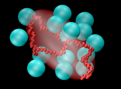
Figure 1: Model of a linear polymer coil (red chain) approximated as a general ellipsoid that fluctuates in size and shape according to random-walk statistics and is penetrable by hard-sphere nanoparticles (blue spheres).

To efficiently explore the influence of nanoparticle crowding on the conformations of polymers in good solvents, we adopt a coarse-grained model of a polymer as a fluctuating ellipsoid whose shape distribution is governed by the gyration tensor of a self-avoiding walk (Fig. 1):

$${\bf T}~{}=~{}\frac{1}{N}\sum_{i=1}^{N}{\bf r}_{i}~{}{\bf r}_{i}~{},$$ (1)

where ${\bf r}_{i}$ is the position relative to the center of mass of segment (step) $i$ of $N$ total segments. The eigenvalues of the gyration tensor – $\Lambda_{1}$, $\Lambda_{2}$, $\Lambda_{3}$ in three dimensions – determine the radius of gyration of the polymer in a particular conformation:

$$R_{p}=\left(\frac{1}{N}\sum_{i=1}^{N}r_{i}^{2}\right)^{1/2}=\sqrt{\Lambda_{1}+\Lambda_{2}+\Lambda_{3}}~{}.$$ (2)

(For reference, the gyration tensor relates to the moment of inertia tensor ${\bf I}$ via ${\bf T}=R_{p}^{2}{\bf 1}-{\bf I}$, with unit tensor ${\bf 1}$.) The root-mean-square (rms) radius of gyration, which can be measured in scattering experiments, is given by

$$R_{g}=\sqrt{\left\langle R_{p}^{2}\right\rangle}=\sqrt{\left\langle\Lambda_{1}+\Lambda_{2}+\Lambda_{3}\right\rangle}~{},$$ (3)

where the angular brackets denote an ensemble average over polymer conformations.

If the ensemble average in Eq. (3) is defined relative to a frame of reference that rotates with the polymer’s principal axes and, furthermore, the principal axes are labelled to preserve the order of the eigenvalues from largest to smallest ($\Lambda_{1}>\Lambda_{2}>\Lambda_{3}$), then the average tensor describes an anisotropic object Rudnick and Gaspari (1986, 1987). The eigenvalues of the gyration tensor define an ellipsoid,

$$\frac{x^{2}}{\Lambda_{1}}+\frac{y^{2}}{\Lambda_{2}}+\frac{z^{2}}{\Lambda_{3}}=3~{},$$ (4)

where $(x,y,z)$ are the coordinates of a point on the surface and the eigenvalues relate to the principal radii $R_{i}$ via $\Lambda_{i}=R_{i}^{2}/3$ ($i=1,2,3$). This general ellipsoid is a coarse-grained representation of the average shape of the polymer (e.g., the tertiary structure of a biopolymer). Each triplet of eigenvalues $\{\Lambda_{1},\Lambda_{2},\Lambda_{3}\}$ characterizes a unique polymer conformation and ellipsoid shape.

In the absence of crowders, a three-dimensional SAW, modeling conformations of a linear polymer in a good solvent, has an average shape (eigenvalue) distribution determined by Monte Carlo simulations Sciutto (1996) to be accurately described by a probability distribution,

$$P_{0}(\Lambda_{1},\Lambda_{2},\Lambda_{3})=\prod_{i=1}^{3}P_{i0}(\Lambda_{i})~{},$$ (5)

where the three factors are given by

$$P_{i0}(\Lambda_{i})=\frac{1}{\Gamma(\nu_{i})}\frac{\nu_{i}}{\alpha_{i}}\left(\frac{\nu_{i}\Lambda_{i}}{\alpha_{i}}\right)^{\nu_{i}-1}\exp\left(-\frac{\nu_{i}\Lambda_{i}}{\alpha_{i}}\right)$$ (6)

and $\alpha_{i}$ and $\nu_{i}$ are fit parameters, tabulated in Table 1 for polymer chains of length $N=10^{4}$. The factorized form of Eq. (5) assumes independent eigenvalues – aside from the ordering condition – an assumption that proves accurate for sufficiently long polymers, with the exception of rare conformations in which an extreme extension in one direction can affect the probability of an extension in an orthogonal direction.

Table 1: Parameters for shape distribution in Eq. (6) Sciutto (1996) for polymer chains of length $N=10^{4}$.

eigenvalue $i$	$\alpha_{i}$	$\nu_{i}$	$\Gamma(\nu_{i})$
1	7591.0120	3.35505	2.84226
2	1604.3861	4.71698	15.8132
3	544.16323	5.84822	92.8188

Table 2: Parameters for shape distribution in Eq. (7).

eigenvalue $i$	$a_{i}$	$b_{i}$	$c_{i}$
1	11847.9	2.35505	22.3563
2	1.11669$\times 10^{9}$	3.71698	148.715
3	1.06899$\times 10^{14}$	4.84822	543.619

An uncrowded SAW polymer of $N$ segments, each of (Kuhn) length $l$, has rms (average) radius of gyration $R_{g}(0)=CN^{\nu}l$, with Flory exponent $\nu=0.588$ and amplitude $C=0.44108$ Sciutto (1996). For comparison, in a $\theta$ solvent, $R_{g}(0)=\sqrt{N/6}~{}l$. Since the gyration tensor eigenvalues increase with $N$ in proportion to $N^{2\nu}$, it is convenient to define scaled eigenvalues, $\lambda_{i}\equiv\Lambda_{i}/(N^{\nu}l)^{2}$, in terms of which the shape distribution can be expressed as

$$P_{i0}(\lambda_{i})=a_{i}\lambda_{i}^{b_{i}}\exp(-c_{i}\lambda_{i})~{},$$ (7)

where the parameters $a_{i}$, $b_{i}$, and $c_{i}$, derived from $\alpha_{i}$ and $\nu_{i}$, are tabulated in Table 2. The individual eigenvalue distributions differ somewhat from the factors in Eqs. (6) and (7). Each is obtained from the parent distribution [Eq. (5)] by integrating over the other two eigenvalues, with limits set by eigenvalue ordering ($\lambda_{1}>\lambda_{2}>\lambda_{3}$):

$$P_{1}(\lambda_{1})=\int_{0}^{\lambda_{1}}d\lambda_{2}\,\int_{0}^{\lambda_{2}}d\lambda_{3}\,P_{0}(\lambda)~{},$$ (8)

$$P_{2}(\lambda_{2})=\int_{\lambda_{2}}^{\infty}d\lambda_{1}\,\int_{0}^{\lambda_{2}}d\lambda_{3}\,P_{0}(\lambda)~{},$$ (9)

$$P_{3}(\lambda_{3})=\int_{\lambda_{3}}^{\infty}d\lambda_{1}\,\int_{\lambda_{3}}^{\lambda_{1}}d\lambda_{2}\,P_{0}(\lambda)~{},$$ (10)

where $\lambda\equiv\{\lambda_{1},\lambda_{2},\lambda_{3}\}$ represents a triplet of scaled eigenvalues. For comparison, Fig. 2 shows the scaled eigenvalue distributions of uncrowded polymers in good and $\theta$ solvents. Note that, accounting for the different scaling factors – $N$ for RW polymers, but $N^{1.176}$ for SAW polymers – the unscaled eigenvalues are significantly larger for a SAW polymer in a good solvent than for a RW polymer in a $\theta$ solvent.

Amidst crowders of volume fraction $\phi_{c}$, the rms radius of gyration $R_{g}(\phi_{c})$ and the principal radii $R_{i}(\phi_{c})$ are related to the scaled eigenvalues via

$$R_{g}(\lambda_{1},\lambda_{2},\lambda_{3},\phi_{c})=\frac{R_{g}(0)}{C}\sqrt{\left\langle\lambda_{1}+\lambda_{2}+\lambda_{3}\right\rangle}$$ (11)

and

$$R_{i}(\lambda_{i},\phi_{c})=\frac{R_{g}(0)}{C}\sqrt{3\lambda_{i}}=3.9269R_{g}(0)\sqrt{\lambda_{i}}~{}.$$ (12)

For comparison, in a $\theta$ solvent, $R_{i}=R_{g}(0)\sqrt{18\lambda_{i}}$ and

$$R_{g}(\phi_{c})=R_{g}(0)\sqrt{6\left\langle\lambda_{1}+\lambda_{2}+\lambda_{3}\right\rangle}.$$ (13)

The principal radii determine the average volume of the ellipsoidal polymer via

$$v_{p}(\lambda_{1},\lambda_{2},\lambda_{3},\phi_{c})=\frac{4\pi}{3}\left\langle R_{1}R_{2}R_{3}\right\rangle.$$ (14)

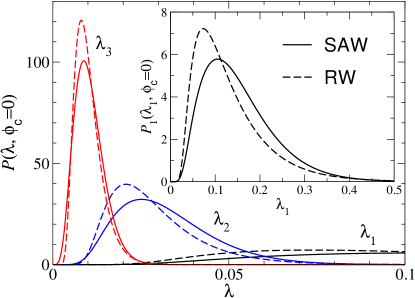
Figure 2: Probability distributions $P(\lambda)$ of scaled gyration tensor eigenvalues $\lambda=\{\lambda_{1},\lambda_{2},\lambda_{3}\}$ of uncrowded polymers ($\phi_{c}=0$) in a good solvent (SAW, solid curves) and in a $\theta$ solvent (RW, dashed curves). Inset: largest eigenvalue $\lambda_{1}$ distributions.

The deviation of a polymer’s average shape from spherical is conveniently quantified by an asphericity parameter Rudnick and Gaspari (1986, 1987), defined as

$$A=1-3\frac{\left\langle\lambda_{1}\lambda_{2}+\lambda_{1}\lambda_{3}+\lambda_{2}\lambda_{3}\right\rangle}{\left\langle(\lambda_{1}+\lambda_{2}+\lambda_{3})^{2}\right\rangle}~{}.$$ (15)

A perfect sphere has all eigenvalues equal and $A=0$, while an elongated object with one eigenvalue much larger than the others has $A\simeq 1$. Crowding agents modify the eigenvalue probability distributions and, in turn, the rms radius of gyration and asphericity of a polymer.

As in our previous studies of crowding of RW polymers in a $\theta$ solvent Lim and Denton (2014, 2016a, 2016b), our model extends the classic Asakura-Oosawa-Vrij (AOV) model of colloid-polymer mixtures Asakura and Oosawa (1954); Vrij (1976), which idealizes nonadsorbing polymers as effective spheres of fixed size (radius of gyration). Although qualitatively describing depletion-induced demixing of colloid-polymer mixtures, the AOV model completely neglects polymer conformational fluctuations, the influence of crowding on polymer size and shape, and the penetrability of polymers by smaller colloids (nanoparticles). We investigate polymer crowding within an extended model of polymer-nanoparticle mixtures that includes all of these features.

II.2 Polymer Penetration Model

To allow for penetration of polymers by crowders, we further extend the AOV model, following previous work Lim and Denton (2014, 2016a, 2016b); Schmidt and Fuchs (2002), by defining an average penetration free energy $\varepsilon$ that represents the average loss in conformational entropy of a polymer upon penetration by a hard-nanosphere crowder of radius $R_{c}$ (see Fig. 1). The dependence of $\varepsilon$ on $q$ can be motivated from a simple scaling argument for an uncrowded polymer in the $N\to\infty$ ($q\gg 1$) limit de Gennes (1979). Given that $\varepsilon$ should be proportional to both the fraction of polymer volume occupied by the nanosphere and the number of polymer segments, we make the scaling ansatz,

$$\beta\varepsilon\sim\frac{R_{c}^{3}}{v_{p}}~{}Y(q)~{},$$ (16)

where the scaling function $Y(q)$ is proportional to $N$. Since $N\sim[R_{g}(0)]^{1/\nu}$ in a good solvent, it follows that $Y(q)\sim q^{1/\nu}$, which implies

$$\beta\varepsilon\sim\frac{R_{c}^{3}}{v_{p}}~{}q^{1/\nu}\sim\frac{R_{g}^{3}(0)}{v_{p}}~{}q^{1/\nu-3}~{},$$ (17)

where $q\equiv R_{g}(0)/R_{c}$ is the uncrowded polymer-to-crowder size ratio. For a SAW polymer in a good solvent at temperature $T$, polymer field theory Eisenriegler et al. (1996); Hanke et al. (1999); Eisenriegler (2000); Eisenriegler et al. (2003) predicts $\nu=0.588$ and, in the limit in which the crowders are much smaller than the polymers ($q\gg 1$):

$$\beta\varepsilon\simeq\frac{18.4R_{g}^{3}(0)}{v_{p}q^{1.29932}}~{}.$$ (18)

For $q\lesssim 1$, nanosphere insertions are so costly in free energy that the polymer is practically impenetrable. Crowders then influence the polymer shape mostly from outside. Conversely, for $q\gg 1$, penetration is less costly and crowding can occur from both inside and outside the polymer. If the polymer were approximated as a sphere of fixed radius, we would have $v_{p}=(4\pi/3)R_{g}^{3}(0)$ and

$$\beta\varepsilon\simeq\frac{4.4}{q^{1.29932}}~{},$$ (19)

an expression that has been used in previous studies of colloid-polymer mixtures in the $q\gg 1$ limit Bolhuis et al. (2003). In our study, however, we used the more general expression of Eq. (18), which applies to a polymer of arbitrary shape. In comparison, for a RW polymer, $\beta\varepsilon\simeq 4\pi R_{g}^{3}(0)/(qv_{p})$, reducing to $\beta\varepsilon\simeq 3/q$ in the spherical polymer model.

The coarse-grained ellipsoidal polymer model should be reasonable if, in the time required for the crowders to significantly change their configuration, the polymer has sufficient time to equilibrate by visiting a representative sample of its possible conformations. We must then assume a separation of time scales between diffusion of crowders and conformational rearrangement of the polymer. For purposes of a rough estimate, we assume that a statistically independent configuration of crowders is achieved when each crowder diffuses a distance comparable to its diameter, while the polymer conformation equilibrates in the time it takes for each segment to diffuse a distance comparable to the segment length. Equating these distances – presuming similar diffusion rates – gives a lower limit on the allowed size of a crowder (upper limit on $q$) for which the model is reasonable. This simple estimate yields $q\simeq\sqrt{N/6}$ for a RW polymer and $q\simeq CN^{\nu}$ for a SAW polymer. Thus, for most practical purposes, and certainly for the systems considered in Sec. IV, the coarse-grained ellipsoidal polymer model is quite justified.

III Methods

III.1 Monte Carlo Simulation

Adapting methods developed in previous studies of polymer crowding Lim and Denton (2014, 2016a, 2016b), we simulated a single ellipsoidal polymer, fluctuating in conformation according to the model described in Sec. II.1, immersed in a fluid of hard nanospheres. In the canonical ensemble, with fixed numbers of particles at constant temperature in a cubic cell of fixed volume with periodic boundary conditions, we implemented a variation of the Metropolis Monte Carlo (MC) algorithm. Trial displacements of nanospheres and polymers were performed by translating the center of a particle at position $(x,y,z)$ to a new position $(x+\Delta x,y+\Delta y,z+\Delta z)$, where $\Delta x$, $\Delta y$, and $\Delta z$ were chosen independently and randomly in the range $[-0.2R_{c},0.2R_{c}]$.

Trial displacements of polymers were coupled with trial rotations and shape changes as a single composite move. To ensure uniform sampling of the polymer orientation, defined by a unit vector ${\bf u}$ aligned with the long axis of the ellipsoid, we generated a new orientation ${\bf u}_{\rm new}$ from an old orientation ${\bf u}_{\rm old}$ via Frenkel and Smit (2001)

$${\bf u}_{\rm new}=\frac{{\bf u}_{\rm old}+\tau{\bf v}}{|{\bf u}_{\rm old}+\tau{\bf v}|}~{},$$ (20)

where ${\bf v}$ is a randomly oriented unit vector and the tolerance $\tau$ was chosen randomly in the range $[-0.1,0.1]$. Trial variations in polymer shape were performed by changing one set of gyration tensor eigenvalues $\lambda_{\rm old}=\{\lambda_{1},\lambda_{2},\lambda_{3}\}$ to a new set $\lambda_{\rm new}=\{\lambda_{1}+\Delta\lambda_{1},\lambda_{2}+\Delta\lambda_{2},\lambda_{3}+\Delta\lambda_{3}\}$, where $\Delta\lambda_{1}$, $\Delta\lambda_{2}$, and $\Delta\lambda_{3}$ were chosen independently and randomly in the ranges $[-0.01,0.01]$, $[-0.003,0.003]$, and $[-0.001,0.001]$. A trial move (displacement, rotation, and shape change) was accepted with probability

$${\cal P}_{\rm acc}=\min\left\{\frac{P_{0}(\lambda_{\rm new})}{P_{0}(\lambda_{\rm old})}e^{-\beta\Delta F},~{}1\right\}~{},$$ (21)

where $\Delta F$ is the change in free energy resulting from the change in number of particle overlaps. For the polymer-nanosphere penetration energy, we used Eq. (18) with the polymer volume predicted by free-volume theory. While in principle we should iterate until $v_{p}$ computed from the simulation equals $v_{p}$ predicted by the theory, in practice the theory proved sufficiently accurate that no iterations were required. A trial move resulting in overlap of hard nanospheres (yielding infinite $\Delta F$) was immediately rejected. A move that creates/eliminates a polymer-nanosphere overlap yields $\Delta F=\pm\varepsilon$ (see Sec. II.2).

During a simulation, we checked whether a trial move resulted in overlap of a nanosphere with the polymer. For each candidate – identified as a nanosphere whose center lies inside a sphere centered on the ellipsoid of radius equal to the sum of the nanosphere radius and the longest principal radius of the ellipsoid – we diagnosed overlap by computing the closest distance between the nanosphere center and the surface of the ellipsoid, which involves computing the roots of a 6th-order polynomial Hart (1994). After an accepted change in polymer conformation, we reordered the eigenvalues by size. During each simulation, we averaged over MC steps, a step being defined as a trial displacement of every nanosphere and a trial change in polymer conformation, to compute ensemble averages of eigenvalue distributions and polymer geometric properties (see Sec. IV). We coded our simulations in Java within the Open Source Physics Library Gould et al. (2006). Figure 3 shows a typical snapshot from a simulation.

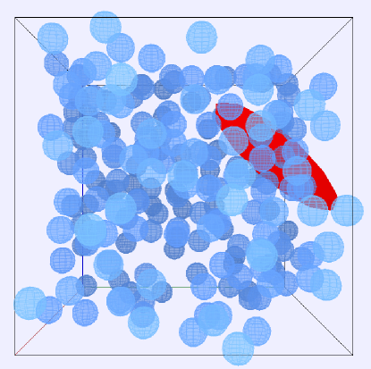
Figure 3: Snapshot of a simulation of $N_{n}=216$ nanospheres (blue spheres) and one polymer (red ellipsoid) in a cubic simulation cell. The rms radius of gyration of the uncrowded polymer equals five times the nanosphere radius ($q$=5).

III.2 Free-Volume Theory of Crowding

To guide choices of system parameters and to help interpret our simulation results, we adapted a free-volume theory previously developed for colloid-polymer mixtures Lim and Denton (2014, 2016a, 2016b). The theory generalizes the theory of Lekkerkerker et al. Lekkerkerker et al. (1992) from the AOV model Asakura and Oosawa (1954); Vrij (1976) of hard, spherical polymers to a model of soft, penetrable, aspherical polymers, as described in Sec. II.

The free-volume theory approximates the mean value of a quantity $Q(\lambda)$, averaged over polymer shapes, by

$$\left\langle Q\right\rangle=\int_{0}^{\infty}d\lambda_{1}\,\int_{0}^{\lambda_{1}}d\lambda_{2}\,\int_{0}^{\lambda_{2}}d\lambda_{3}\,Q(\lambda)P(\lambda,\phi_{c})~{},$$ (22)

where

$$P(\lambda,\phi_{c})=\frac{\alpha(\lambda,\phi_{c})}{\alpha_{\rm eff}(\phi_{c})}P_{0}(\lambda)$$ (23)

is the shape probability distribution of the crowded polymer, $\alpha(\lambda,\phi_{c})$ is the free-volume fraction of a polymer of shape $\lambda\equiv\{\lambda_{1},\lambda_{2},\lambda_{3}\}$ amidst hard nanospheres of average volume fraction $\phi_{c}$, and

$$\alpha_{\rm eff}(\phi_{c})=\int_{0}^{\infty}d\lambda_{1}\,\int_{0}^{\lambda_{1}}d\lambda_{2}\,\int_{0}^{\lambda_{2}}d\lambda_{3}\,\alpha(\lambda,\phi_{c})P_{0}(\lambda)$$ (24)

is the effective free-volume fraction, averaged over polymer shapes. Note that the limits of the eigenvalue integrals in Eqs. (22) and (24) are chosen to respect the eigenvalue ordering ($\lambda_{1}>\lambda_{2}>\lambda_{3}$). Previous studies of crowding of RW (ideal) polymers Lim and Denton (2014, 2016a, 2016b) did not impose eigenvalue ordering. While this simple approximation proves very accurate and efficient for RW polymers, it turns out to be less accurate for SAW polymers, increasingly so with increasing crowder volume fraction.

According to the Widom particle insertion theorem Widom (1963), the free-volume fraction is related to the average work $W$ required to insert a polymer of shape $\lambda$ into a sea of hard spheres of volume fraction $\phi_{c}$ via

$$\alpha(\lambda,\phi_{c})=\exp[-\beta W(\lambda,\phi_{c})]~{}.$$ (25)

The average insertion work or, equivalently, the free energy required to distort the hard-sphere fluid and create the volume and interfacial area sufficient to accommodate the polymer, can be expressed as

$$W(\lambda,\phi_{c})=p(\phi_{c})v_{p}(\lambda)+\oint_{S}dS\,\gamma(\phi_{c},{\bf r})~{},$$ (26)

where $p$ and $\gamma$ are the pressure and interfacial tension of the hard-sphere fluid, respectively, $v_{p}(\lambda)$ is the volume of the polymer, and the integral is over a closed surface $S$, defined by the surface of the ellipsoidal polymer and parametrized by surface position vector ${\bf r}$. This expression conveniently and conceptually separates thermodynamic properties of the hard-sphere fluid from geometric properties of the polymer.

Assuming a smooth interface between the polymer and the hard-sphere fluid, the interfacial tension, which depends on the curvature of the interface – dictated by the polymer shape – can be expanded in powers of the mean curvature

$$K({\bf r})=\frac{1}{2}\left(\frac{1}{R_{1}({\bf r})}+\frac{1}{R_{2}({\bf r})}\right)$$ (27)

and the Gaussian curvature

$$H({\bf r})=\frac{1}{R_{1}({\bf r})R_{2}({\bf r})}~{},$$ (28)

where $R_{1}({\bf r})$ and $R_{2}({\bf r})$ are the local radii of curvature at a point ${\bf r}$ on the interface. Thus,

$$\gamma(\phi_{c},{\bf r})=\gamma_{\infty}(\phi_{c})+\kappa(\phi_{c})K({\bf r})+\bar{\kappa}(\phi_{c})H({\bf r})+\cdots~{},$$ (29)

where $\gamma_{\infty}$ is the interfacial tension of a flat interface (with infinite radii of curvature) and the coefficients $\kappa(\phi_{c})$ and $\bar{\kappa}(\phi_{c})$ are bending rigidities of the hard-sphere fluid, which depend only on the hard-sphere volume fraction. Substituting Eq. (29) into Eq. (26) and integrating over eigenvalues yields the curvature expansion of the insertion work:

$$W(\lambda,\phi_{c}) = p(\phi_{c})v_{p}(\lambda)+\gamma_{\infty}(\phi_{c})a_{p}(\lambda)$$ (30)

$$+ \kappa(\phi_{c})c_{p}(\lambda)+2\pi\bar{\kappa}(\phi_{c})+\cdots~{},$$

where $a_{p}(\lambda)$ is the surface area of the ellipsoidal polymer,

$$c_{p}(\lambda)=\oint_{S}dS\,K({\bf r})$$ (31)

is the integrated mean curvature, and we have exploited the Gauss-Bonnet theorem:

$$\oint_{S}dS\,H({\bf r})=2\pi\chi~{},$$ (32)

where the Euler characteristic $\chi=1$ for an ellipsoid. Substituting Eq. (30) into Eq. (25) and neglecting higher-order terms in the curvature expansion yields an approximation for the polymer free-volume fraction:

$$\alpha(\lambda,\phi_{c}) = \exp\{-\beta[p(\phi_{c})v_{p}(\lambda)+\gamma_{\infty}(\phi_{c})a_{p}(\lambda)$$ (33)

$$+ \kappa(\phi_{c})c_{p}(\lambda)+2\pi\bar{\kappa}(\phi_{c})]\}~{}.$$

In the limit of an infinitesimally small (point-like) polymer coil ($\lambda\to 0$), $v_{p}(\lambda)$, $a_{p}(\lambda)$, and $c_{p}(\lambda)$ all tend to zero and the free-volume fraction then reduces to $1-\phi_{c}$, implying that

$$\bar{\kappa}(\phi_{c})=-\frac{k_{\rm B}T}{2\pi}\ln(1-\phi_{c})~{}.$$ (34)

Finally, to incorporate the penetrability of the polymers, the crowder volume fraction is replaced by an effective volume fraction, $\phi_{c}^{\prime}=\phi_{c}(1-e^{-\beta\varepsilon})$ Lim and Denton (2014, 2016a, 2016b); Schmidt and Fuchs (2002). Combining Eqs. (33) and (34) yields the final approximation for the polymer free-volume fraction:

$$\alpha(\lambda,\phi_{c}) = (1-\phi_{c}^{\prime})\exp\{-\beta[p(\phi_{c}^{\prime})v_{p}(\lambda)+\gamma_{\infty}(\phi_{c}^{\prime})a_{p}(\lambda)$$ (35)

$$+ \kappa(\phi_{c}^{\prime})c_{p}(\lambda)]\}~{},$$

from which mean values follow via Eqs. (22)-(24).

With knowledge of $p(\phi_{c})$, $\gamma_{\infty}(\phi_{c})$, and $\kappa(\phi_{c})$ in the curvature expansion of the insertion work [Eq. (30)], the free-volume theory can be implemented to predict the dependence of polymer size and shape on crowding by a hard-sphere fluid. For example, the radius of gyration $R_{g}(\phi_{c})$ can be explicitly computed from

$$R_{g}(\phi_{c})=\frac{R_{g}(0)}{C}\int d\lambda\,P(\lambda,\phi_{c})\sqrt{\lambda_{1}+\lambda_{2}+\lambda_{3}}~{}.$$ (36)

To compute the results reported in Sec. IV, we used the accurate Carnahan-Starling expressions for the hard-sphere fluid properties Oversteegen and Roth (2005); Hansen and McDonald (2006):

$$\beta p(\phi_{c}) = \frac{3\phi_{c}}{4\pi R_{c}^{3}}\frac{1+\phi_{c}+\phi_{c}^{2}-\phi_{c}^{3}}{(1-\phi_{c})^{3}}$$

$$\beta\gamma_{\infty}(\phi_{c}) = \frac{3}{4\pi R_{c}^{2}}\left[\frac{\phi_{c}(2-\phi_{c})}{(1-\phi_{c})^{2}}+\ln(1-\phi_{c})\right]$$

$$\beta\kappa(\phi_{c}) = \frac{3\phi_{c}}{R_{c}(1-\phi_{c})}~{}.$$ (37)

For the integrated mean curvature, we numerically evaluated the integral in Eq. (31) over a grid of eigenvalues and stored the results in a look-up table for later access.

IV Results

IV.1 Simulation Protocol

For several choices of uncrowded polymer-to-crowder size ratio $q$ and crowder volume fraction $\phi_{c}$, we performed simulations of a polymer coil (modeled as a fluctuating, penetrable ellipsoid) and $N_{n}$=216 nanosphere crowders, initialized on a cubic lattice ($6\times 6\times 6$ array). After an equilibration stage of 5 $\times$ $10^{4}$ MC steps, we collected statistics for the three eigenvalues of the gyration tensor at intervals of $10^{3}$ MC steps for $10^{4}$ intervals. For each parameter combination, we ran five independent simulations and averaged over runs to obtain statistical errors. We ran test simulations for longer times and larger systems to ensure that the system had reached equilibrium and that finite-size effects were negligible. From the raw eigenvalue data, we obtained probability distributions [Eq. (23)] as histograms (see Figs. 4 and 5) and computed average polymer geometric properties: radius of gyration [Eq. (11)], volume [Eq. (14)], and asphericity [Eq. (15)] (see Figs. 6 and 7).

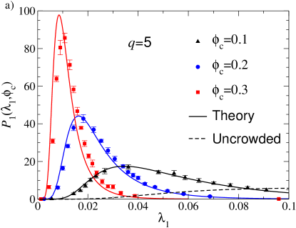
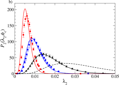
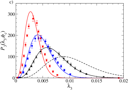
Figure 4: Eigenvalue probability distributions ($\lambda_{1}>\lambda_{2}>\lambda_{3}$) of gyration tensor of a crowded polymer coil in a good solvent, modeled as a fluctuating, penetrable ellipsoid, governed by self-avoiding-walk statistics. Simulation data (symbols) are compared with predictions of free-volume theory (solid curves) for a single polymer, with uncrowded rms radius of gyration equal to five times the nanoparticle radius ($q=5$), amidst $N_{n}$ = 216 hard nanosphere crowders of volume fraction $\phi_{c}=0.1$ (triangles), 0.2 (squares), and 0.3 (circles). Dashed curves show uncrowded ($\phi_{c}=0$) distributions.

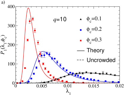
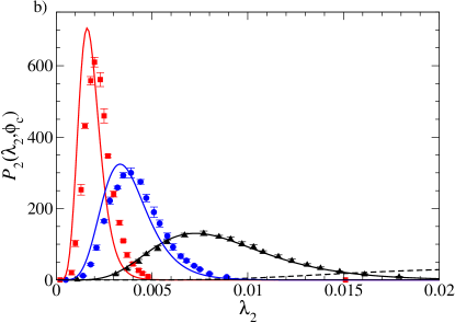
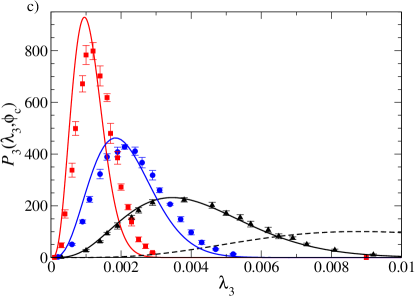
Figure 5: Same as Fig. 4, but for uncrowded polymer-to-nanosphere size ratio $q=10$. Notice changes in horizontal and vertical scales.

IV.2 Comparison of SAW and RW Polymers of Equal Uncrowded Size

We first present and discuss results that illustrate the influence of solvent quality on conformations of crowded SAW and RW polymers having the same uncrowded size (radius of gyration). Figures 4 and 5 show our simulation results for the eigenvalue probability distributions for $q=5$ and $q=10$, respectively, over a range of crowder volume fraction. Also shown are predictions of our free-volume theory. Simulation and theory are in reasonable agreement, deviations increasing with $\phi_{c}$ as polymer-crowder correlations strengthen, and both predict progressive shifts to lower eigenvalues (smaller principal radii) and narrowing of the distributions with increasing crowder volume fraction. These results reveal that, with increasing $\phi_{c}$, not only do polymer coils tend to contract along each principal axis, but also fluctuations in size and shape are suppressed – more so for $q=10$ than for $q=5$. The slightly larger deviations between theory and simulation at larger $q$ – evident especially at higher $\phi_{c}$ – reflect limitations of the theory associated with neglecting higher-order terms in the curvature expansion of the interfacial tension [Eqs. (29) and (30)]. These deviations propagate forward and affect the predicted size and shape of the crowded polymer, which depend on averages over the eigenvalue distributions.

Figure 6 illustrates the influence of crowding on geometric properties of a polymer coil. The average radius of gyration, volume, and asphericity of the polymer all decrease monotonically with increasing crowder volume fraction. Polymers of uncrowded $R_{g}$ equal to the crowder radius ($q=1$) are relatively insensitive to crowding, experiencing only a 15% reduction in size at $\phi_{c}=0.3$, while larger polymers ($q=5$, 10) contract significantly more than smaller polymers at the same $\phi_{c}$. The crowding effect predicted at $q=1$, though relatively weak, is stronger than that determined from the experiments of ref. Palit et al. (2017), in which no significant change in radius of gyration was observed over the same range of $\phi_{c}$. Although its source is unclear, this quantitative disagreement may result from some mismatch between our model and the experimental system. It may be, for example, that the conformational statistics exhibited by the polymer (PEG) in water are not quite those of a SAW, or that the interactions between crowding agents (Ficoll 70) differ from hard-sphere interactions, or that the polymer-crowder interactions are not purely entropic.

The tendency of polymer contraction to increase with increasing $q$, at fixed $\phi_{c}$, is a result of the free energy cost associated with penetration of a polymer by crowders. Figure 7 illustrates more directly the variation of polymer geometry with size ratio, showing that radius of gyration, volume, and asphericity all decrease monotonically with increasing $q$. Evidently, the larger the polymer relative to the crowder, the more severe the influence of crowding on polymer conformation. This trend can be explained by the fact that the total penetration energy scales as $q^{1/\nu}=q^{1.7}$ for a given $\phi_{c}$. The latter scaling follows from the scaling of the penetration energy as $q^{1/\nu-3}$ [Eq. (17)] and the number of penetrating nanospheres per polymer as $q^{3}$. While our results for the dependence of $R_{g}$ on $\phi_{c}$ and $q$ are qualitatively consistent with the measurements of Palit et al. Palit et al. (2017) for aqueous solutions of PEG and Ficoll 70, in that polymer contraction increases monotonically with increasing $q$ and $\phi_{c}$, quantitative differences exist. Future studies may determine whether the discrepancies can be accounted for by the particular chain statistics of PEG in water or by non-hard-sphere interactions between the Ficoll 70 crowders or by other limitations of our model.

Also shown in Figs. 6 and 7 are corresponding predictions of free-volume theory for both SAW and RW polymers. Results for SAW polymers from simulation and theory generally agree closely, as found also in previous studies of RW polymer Lim and Denton (2014, 2016a, 2016b). For clarity of presentation, we do not include here previously reported simulation data for RW polymers, as they are in near-exact agreement with simulation. As noted in Sec. III.1, the output values of $v_{p}$ are sufficiently close to the input values (from free-volume theory) that no iterations between simulation and theory were required. We emphasize that imposing ordering of eigenvalues turns out to have negligible effect on the results for RW polymer, but is more significant for SAW polymer, especially at higher $\phi_{c}$.

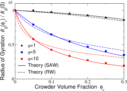
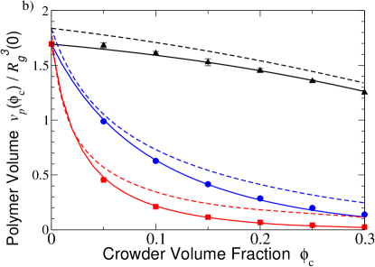
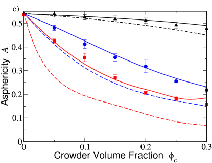
Figure 6: Average geometric properties a polymer (modeled as a fluctuating, penetrable ellipsoid) vs. nanosphere crowder volume fraction $\phi_{c}$: (a) rms radius of gyration, (b) volume, (c) asphericity. Simulation data are shown for SAW polymers of uncrowded polymer-to-nanosphere size ratio $q=1$ (triangles), $q=5$ (circles), and $q=10$ (squares). For some points, error bars are smaller than symbols. Corresponding predictions of free-volume theory are shown for SAW polymers (solid curves) and RW polymers (dashed curves).

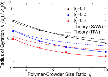
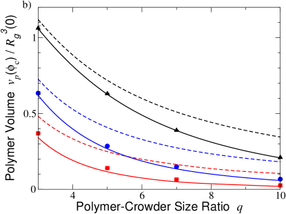
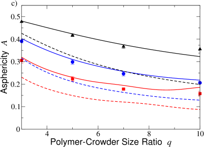
Figure 7: Average geometric properties of a polymer (modeled as a fluctuating, penetrable ellipsoid) vs. uncrowded polymer-to-nanosphere size ratio $q$: (a) radius of gyration, (b) volume, (c) asphericity. Simulation data are shown for SAW polymers and nanosphere crowder volume fraction $\phi_{c}=0.1$ (triangles), $\phi_{c}=0.2$ (circles), and $\phi_{c}=0.3$ (squares). For some points, error bars are smaller than symbols. Corresponding predictions of free-volume theory are shown for SAW polymers (solid curves) and RW polymers (dashed curves).

While polymers in different solvents show qualitatively similar responses to crowding, all geometric measures decreasing with increasing $\phi_{c}$, there are significant quantitative differences. For the same $q$ and $\phi_{c}$, a SAW polymer (in a good solvent) has a consistently smaller volume [Figs. 6b and 7b] and higher asphericity [Figs. 6c and 7c] than a RW polymer (in a $\theta$ solvent). Thus, a SAW polymer in a crowded environment is more compressed and more elongated than a RW polymer of the same uncrowded size (same $q$). The comparison of crowded sizes of SAW and RW polymer is somewhat more complicated. Fig. 6a shows that for $q=1$ the SAW polymer is consistently less contracted over the whole range of crowder volume fraction, while for $q=5$ and $q=10$, the SAW polymer contracts less at lower $\phi_{c}$, but more at higher $\phi_{c}$. This cross-over with increasing $q$ and $\phi_{c}$ in the degree of contraction of SAW and RW polymers reflects a complex interplay between, on the one hand, chain statistics and conformational entropy, and on the other hand, penetration free energy (see Sec. II.2). When we consider, however, polymers of the same segment number (molecular weight), rather than the same uncrowded size, the responses of SAW and RW polymers to crowding are more distinct, as we discuss in the next section.

IV.3 Comparison of SAW and RW Polymers of Equal Segment Number

Thus far, when comparing the crowded conformations (sizes and shapes) of a SAW polymer in a good solvent with those of a RW polymer in a $\theta$ solvent, we have considered polymers of the same uncrowded radius of gyration (same $q$ value). Since the scaling of $R_{g}(0)$ with segment number $N$ depends on the solvent quality de Gennes (1979) (see Sec. II.1), we have implicitly been comparing polymers of different segment numbers. Our predictions, while of fundamental interest and qualitatively consistent with observed trends, may be difficult to compare with experiments in which polymers of the same molecular weight are studied under different solvent conditions. To facilitate more direct comparisons with experiments, we now compare predictions for polymers of equal segment number in good and $\theta$ solvents.

Given the segment (Kuhn) length $l$ of a linear polymer coil, the radius of a spherical crowder, and the size ratio $q_{\scriptscriptstyle\rm RW}$ of a RW polymer in a $\theta$ solvent, the scaling relations (Sec. II.1) determine the size ratio $q_{\scriptscriptstyle\rm SAW}$ of a SAW polymer of equal segment number in a good solvent:

$$q_{\scriptscriptstyle\rm SAW}=C6^{\nu}(R_{c}/l)^{2\nu-1}q_{\scriptscriptstyle\rm RW}^{2\nu}~{}.$$ (38)

As an example, motivated by the recent experiments of Palit et al. Palit et al. (2017), we consider aqueous solutions of PEG and Ficoll 70 crowder. Taking the Kuhn length of PEG in water – considered good solvent conditions at room temperature – as $l=7.6$ Å Lee et al. (2008) (twice the persistence length), the radius of Ficoll 70 as $R_{c}=55$ Å van den Berg et al. (2000), and $q_{\scriptscriptstyle\rm RW}=3$, we obtain $q_{\scriptscriptstyle\rm SAW}\simeq 7$ and $N\simeq 3000$ segments. (For comparison, $q_{\scriptscriptstyle\rm SAW}=1$ translates into $q_{\scriptscriptstyle\rm RW}\simeq 0.6$ and $N\simeq 120$.)

Figure 8 compares the geometric properties of this polymer in good and $\theta$ solvents. With increasing crowder volume fraction, the influence of crowding on conformations of a polymer of a given molecular weight – quantified by radius of gyration, volume, and asphericity – is consistently stronger in a good solvent than in a $\theta$ solvent. These trends are not surprising, given our general understanding that crowding effects become more prominent with increasing $q$, and considering that $q_{\scriptscriptstyle\rm SAW}$ here exceeds $q_{\scriptscriptstyle\rm RW}$ by more than a factor of two. What is perhaps most notable is that the average polymer shape (asphericity), while strongly dependent on crowder volume fraction, is relatively insensitive – compared with average polymer size – to a change in solvent quality. It is worth noting that our $R_{g}$ vs. $\phi_{c}$ data have a sign of curvature (positive) that is opposite that of the experimental data Palit et al. (2017). Quantitative comparisons are complicated, however, by the relative simplicity of our model and the fact that, for given molecular weights of PEG, the measured uncrowded radii of gyration obey neither RW nor SAW chain statistics.

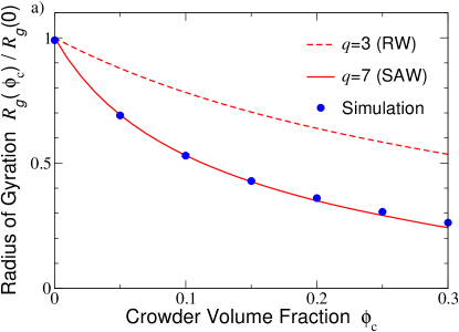
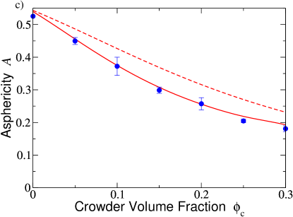
Figure 8: Average geometric properties of PEG (modeled as a fluctuating, penetrable ellipsoid) vs. volume fraction $\phi_{c}$ of Ficoll 70 crowders (modeled as hard spheres) in water. (a) radius of gyration, (b) volume, and (c) asphericity of the polymer. Simulation data (symbols) and theoretical predictions (solid curves) for SAW model of a polymer in a good solvent with $q\simeq 7$ are compared with predictions for RW model of the same polymer in a $\theta$ solvent with $q=3$ (dashed curves). For both cases, the polymer contains $N\simeq 3000$ segments, comparable to the experiments of ref. Palit et al. (2017).

V Conclusions

To summarize, we have investigated the dependence on solvent quality of polymer conformations in crowded environments. For computational efficiency and conceptual simplicity, we modeled a polymer coil as an effective ellipsoid whose size and shape fluctuate according to the underlying statistics of random walks. Specifically, fluctuations of the principal radii follow the probability distributions of the gyration tensor eigenvalues of either a self-avoiding walk – for a polymer in a good solvent – or a random walk – for a polymer in a $\theta$ solvent. Crowders are modeled as hard-sphere nanoparticles that mutually interact via a hard-sphere pair potential and are allowed to penetrate the volume enclosed by polymers with an average free energy cost predicted by field theory.

We implemented this coarse-grained model of polymer-crowder mixtures via Monte Carlo simulation and free-volume theory for polymers in good and $\theta$ solvents. As input to both simulations and theory, we used eigenvalue distributions previously determined from molecular simulations of random walks. Our simulation data indicate that, with increasing crowder volume fraction and uncrowded polymer-to-crowder size ratio $q$, polymers become smaller and more compact (i.e., more spherical), in good agreement with predictions of free-volume theory. While the conformations of SAW and RW polymers display similar qualitative trends, they exhibit significant quantitative differences. For polymers that are equal in either radius of gyration or segment number, the influence of crowding is consistently stronger in a good solvent than in a $\theta$ solvent. This dependence on solvent quality can be attributed to the important role of segment self-avoidance on both the statistics and the penetrability of a polymer chain in a good solvent. Our prediction can be experimentally tested by measuring the radius of gyration of polymers in dilute and crowded solutions under different solvent conditions, achievable by varying either temperature or concentration of a cosolvent.

The model considered here, in which polymer shapes are governed by random-walk statistics and crowders are treated as inert hard spheres, has the virtue of isolating and highlighting the role of excluded volume in polymer crowding. Quantitative description of many real systems, however, may require incorporating intra-chain interactions (chain enthalpy), with appropriate uncrowded eigenvalue distributions, crowder-crowder interactions, and internal structure of crowders. For example, real biopolymers may follow different chain statistics, while specific crowders may be compressible and, if charged, may mutually interact by screened electrostatic potentials. Moreover, while our model of mobile polymers and crowders is designed to apply most closely to macromolecular crowding of biopolymers in cellular environments, a model of polymers amidst fixed obstacles may be more applicable to polymer nanocomposite materials. Future work should investigate the dependence of polymer conformations on chain statistics, crowder-crowder interactions, crowder structure, and crowder mobility. Further simulations of more explicit (e.g., bead-spring) models of polymers in crowded environments Denesyuk and Thirumalai (2011, 2013a, 2013b); Kang et al. (2015) also would help to test, calibrate, and refine the coarse-grained ellipsoidal polymer model.