Bandgaps in two-dimensional high-contrast periodic elastic beam lattice materials

Abstract.

We consider elastic waves in a two-dimensional periodic lattice network of Timoshenko-type beams. We show that for general configurations involving certain highly-contrasting components a high-contrast modification of the homogenization theory is capable of accounting for bandgaps, explicitly relating those to low resonant frequencies of the “soft” components. An explicit example of a square-periodic network of beams with a single isolated resonant beam within a periodicity cell is considered in detail.

1. Introduction

Macroscopic properties of lattice materials, and their static and dynamic responses have been of a considerable recent interest. In particular, Phani, Woodhouse and Fleck [18] studied wave propagation for certain lattice topologies and associated phenomena of frequency bandgaps and spatial filtering (wave directionality) by adopting Floquet-Bloch’s principles for lattices modeled as a network of Timoshenko beams using the finite element method. Long-wavelength asymptotes to the resulting dispersion curves were found to be in good agreement with those based on homogenization (effective medium) theories, however the range of validity of the latter was found to be restricted to low frequencies i.e. below the frequencies where the bandgaps may be observed.

In the present work we argue however that for periodic elastic beam configurations involving certain highly-contrasting components, a high-contrast modification of the homogenization theory is capable of accounting both for bandgaps and for certain forms of polarization filtering, with the former explicitly related to (low) resonance frequencies of the “soft” components. As a result of the high contrast, and as opposed to the classical homogenization, under a naturally chosen micro-resonant scaling the asymptotic description of the wave processes remains intrinsically two-scale, which in fact gives rise to the above effects. We emphasize that the mathematical approach adopted here is rigorous in the sense that it does not rely on any further assumptions, and provides approximations for entities of interest for the underlying Floquet-Bloch waves and in particular for the bandgaps with a controllably small error for a sufficiently high value of the parameter of the contrast.

Without attempting here a comprehensive review of the relevant literature, some related ideas for two-phase high-contrast and generally highly-anisotropic periodic elastic composites were discussed in [20] with some examples of both frequency gaps and of long-wavelength “directional localization”, following mathematical ideas of [25, 26]. Related developments specifically for high-contrast linear elasticity include those by [6], [27], [10], and for high-contrast graphs but outside elasticity by [9]. The derived macroscopic equations in the bandgap regime allow interpretation in terms of negative effective density (or sign-indefinite anisotropic density in case of “weak” gaps) for some frequency ranges. Some related general ideas are found in [24], and in a specific context of high-frequency periodic homogenization this was probably first observed by [2, 1] and developed further by [8] and [3], among others. Some related general mathematical issues for two-scale homogenization of systems of partial differential equations with partially degenerating periodic coefficients were recently studied by us in [11].

From the mathematical perspective, the case of high-contrast Timoshenko-type elastic beam networks appears of additional interest (and indeed of a non-trivial additional challenge to us) for the non-trivial effect of microscopic rotations on the two-scale limit asymptotic behavior. In particular, the three microscopic degrees of freedom (two displacements and a rotation) generate, for a given frequency, up to three propagating Bloch modes. However, in the chosen (two-scale) high-contrast asymptotic regime, only up to two modes can propagate, as in the conventional two-dimensional (2-D) elasticity: the rotational degree of freedom remains purely microscopic, but nevertheless still affects the macroscopic part via the two-scale coupling. The latter is due to the fact that, for a periodically connected stiff component, the homogenized tensor turns out to be conventional 2-D elastic (i.e. with no macroscopic rotational degree of freedom): this is not obvious a priori, and we establish this as a by-product of our analysis. A further related feature of the limit two-scale model is that, due to the coupling between the two above macroscopic modes, in principle the microscopic resonances may not necessarily lead to bandgaps (in contrast to the prototype scalar models of [26]). We show that the gaps nevertheless do appear, at least for particular configurations.

The issues of filtering properties for various models of elastic lattice structures including band gaps have also been intensively studied before, see for example [16] and further references therein, and [15], although to the best of our knowledge not specifically for the high-contrast “micro-resonant” scaling for which, as we argue in this work, the lattice structures with highly-contrasting components provide distinct scenarios for such effects and for their understanding in terms of the underlying lattice resonances. On the other hand, effect of the resonances on the bandgaps has been studied e.g. by [19] for a simple model of a single Timoshenko beam with attached periodic masses and resonators.

The structure of the paper is as follows. In Section 2 we describe a model for wave propagation in a two-dimensional periodic elastic Timoshenko beam network, which is essentially the same as the underlying initial model of rigid-jointed network of beams of [18], but without any further approximations for the fields on the beams and with some high-contrast elements. We then explain how the resonance effect for the soft part leads to a natural scaling for high contrast vs small periodicity. Section 3 executes two-scale asymptotic analysis of the emerging problem, and derives a two-scale limit problem. The limit problem is analyzed in Section 4, which discusses how it reveals the effect of full and partial (weak) band gaps and their relation to the underlying resonances. Section 5 considers an explicit example of a square beam network with isolated resonant beams, where the entities of interest are evaluated analytically, and as a result the existence of both full and “partial” bandgaps is established via a further qualitative argument. The Appendix explicitly calculates the homogenized elasticity tensor for the stiff component in the above example.

2. Periodic beam networks with a high contrast

Similarly to [18], we consider a two-dimensional periodic rigid-jointed network of beams with no pre-stress akin to the one displayed on Fig. 1.

Figure 1. Geometric configuration: a periodic network of beams

Each beam of a length $L$ is modeled as a Timoshenko beam, see e.g. [22], with any of its center-line material points $x$, $-L/2\leq x\leq L/2$, having three degrees of freedom (Fig. 2): longitudinal displacement $u(x)$ along the beam, displacement $v(x)$ in the transverse direction $y$, and the total rotation $\theta(x)$ of the material normal to the undeformed beam about the $z$-axis. (The latter is a combined effect of the rotation $dv/dx$ of the beam and of an additional rotation due to the shear within the beam.)

Figure 2. Timoshenko beam

The resulting kinetic and potential energies per unit thickness of the beam in the $z$-direction, are:

(1) $$T_{b}\,=\,\frac{1}{2}\int_{-L/2}^{L/2}\left[\,\rho\dot{u}^{2}\,+\rho\dot{v}^{2}\,+\,\rho I\dot{\theta}^{2}\right]\,dx,$$

(2) $$U_{b}\,=\,\frac{1}{2}\int_{-L/2}^{L/2}\left[\,E\left(\frac{du}{dx}\right)^{2}\,+\,EI\left(\frac{d\theta}{dx}\right)^{2}\,+\,G\left(\frac{dv}{dx}-\theta\right)^{2}\right]\,dx.$$

Here the positive parameters describe physical and geometrical properties of the beam: $\rho$ is the density of the beam per unit length, $I$ is the second moment of area of the beam divided by its thickness, and $E$ and $G$ characterize mechanical stiffness of the beam in extension and shear, see e.g. [22] and [18] for more details. These parameters may vary from one beam to another within a periodicity cell, however they are assumed to be periodically replicated from one cell to another. Notice that $U_{b}=0$ if and only if $\theta=c_{1}$, $u=c_{2}$ and $v=c_{3}+c_{1}y$ with constant $c_{1}$, $c_{2}$ and $c_{3}$, which corresponds to rigid body motions. The imposed below following [18] condition of rigid joints implies the continuity of the relevant components of displacement as well as the continuity of the rotation $\theta$.

The total kinetic and potential energies within a finite volume $V$ of the network are the sums over all beams within $V$,

$$T\,=\,\sum_{j}T_{b_{j}},\ \ \ \ U\,=\,\sum_{j}U_{b_{j}},$$

and the equations of motion, in the absence of external forces, are derived by applying Hamilton’s variational principle,

(3) $$\delta\int(T\,-\,U)\,dt\,=\,0.$$

The latter, via (1) and (2), can be conveniently written in the following weak form:

$$\sum_{j}\int_{-L_{j}/2}^{L_{j}/2}\left[\,\rho_{j}\ddot{u}_{j}\tilde{u}_{j}\,+\rho_{j}\ddot{v}_{j}\tilde{v}_{j}\,+\,\rho_{j}I_{j}\ddot{\theta}_{j}\tilde{\theta}_{j}\,\,\,\,+\ \ \ \ \ \ \ \ \ \ \ \ \ \ \right.$$

(4) $$\left.\,E_{j}\frac{du_{j}}{dx_{j}}\frac{d\tilde{u}_{j}}{dx_{j}}\,+\,E_{j}I_{j}\frac{d\theta_{j}}{dx_{j}}\frac{d\tilde{\theta}_{j}}{dx_{j}}\,+\,G_{j}\left(\frac{dv_{j}}{dx_{j}}-\theta_{j}\right)\left(\frac{d\tilde{v}_{j}}{dx_{j}}-\tilde{\theta}_{j}\right)\right]\,dx_{j}\,\,=\,\,0.$$

Here the integral identity is required to hold, for any time $t$, for all smooth test functions $(\tilde{u}_{j},\tilde{v}_{j},\tilde{\theta}_{j})$ supported on the graph within $V$, which together with the sought solution $(u_{j},v_{j},\theta_{j})$ satisfy the kinematic continuity conditions at the joints. Namely, at a joint $J$, for all the beams $b_{j}$ connecting to $J$ (denoted $j\in J$), $\theta_{j}$ are continuous and the displacements associated with $u_{j}$ and $v_{j}$ are continuous as well, i.e.

(5) $$\theta_{j}\,=\,\theta_{l}\,\,\mbox{ and }\,\,u_{j}\mbox{\boldmath{$\tau$}}^{(j)}\,+\,v_{j}\mathbf{n}^{(j)}\,=\,u_{l}\mbox{\boldmath{$\tau$}}^{(l)}\,+\,v_{l}\mathbf{n}^{(l)},\,\,\,\mbox{ for all }j,l\in J,$$

where $\mbox{\boldmath{$\tau$}}^{(j)}$ is the unit vector along the beam $b_{j}$ in the direction of the increase of $u_{j}$ and $\mathbf{n}^{(j)}$ is the unit vector in the normal direction of the positive $v_{j}$.

We emphasize here that the chosen microscopic model is essentially identical to the underlying initial model of [18] of rigid-jointed network of beams. In (5), together with the condition of continuity of the displacements (which is natural assuming the joint region is small enough), both require the continuity of the rotations. Notice that the latter continuity is implicitly enforced by [18] via prescribing $\theta$ (as well as the total displacements) at the nodes only and then continuously

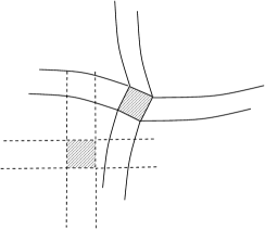
Figure 3. Rigid joint regions, shown as shaded squares for the undeformed (dashed lines) and the deformed (solid lines) junction of four Timoshenko beams

approximating them between the nodes (i.e. on the beams) by particular “shape functions” (Appendix of [18]), within the “exact” Hamilton’s variational framework (3). Our approach remains exact in the sense that it does not involve any such further approximations. The continuity of the rotations appears natural, as it assumes that the rigid joint region is of a small size commensurable with the thickness $d$ of the beams, which is in turn assumed much smaller than the length of the lattice $L$. All the beams, see an illustration on Fig. 3, are assumed bonded to the joint along their undeformed normals and so, as only rigid motion (i.e. translations and rotations) of the joint is allowed, the normals of all the beams in the immediate vicinity of the joint have the same amount of rotation $\theta$. A systematic derivation of such a condition would require asymptotic analysis involving a small parameter of the size of the joint, cf e.g. [13, 17] and/or variational approximations to Hamilton’s principle (3) cf. e.g. [23, 21], which is beyond the scope of the present work. Such a model of rigid joints is often postulated in the literature, e.g. in [14] p. 352, which leads to a mathematically well-posed problem on the resulting network. So we adopt this particular model as a part of our microscopic problem, although our approach can be applied to other models of beam networks as well.

For time-harmonic waves of an angular frequency $\omega$ which may propagate through such an infinite-periodic lattice, in particular for Floquet-Bloch waves, the equation of motion is obtained by formally adopting the time dependence throughout in (4) through the factor $e^{i\omega t}$. Allowing the same notation for the time-harmonic part, i.e. assuming in (4) $u_{j}(x,t)=e^{i\omega t}u_{j}(x)$, etc, transforms (4) into a spectral problem

$$\sum_{j}\int_{-L_{j}/2}^{L_{j}/2}\left[\,E_{j}\frac{du_{j}}{dx_{j}}\frac{d\tilde{u}_{j}}{dx_{j}}\,+\,E_{j}I_{j}\frac{d\theta_{j}}{dx_{j}}\frac{d\tilde{\theta}_{j}}{dx_{j}}\,+\,G_{j}\left(\frac{dv_{j}}{dx_{j}}-\theta_{j}\right)\left(\frac{d\tilde{v}_{j}}{dx_{j}}-\tilde{\theta}_{j}\right)\right]\,dx_{j}\,\,=$$

(6) $$\omega^{2}\,\sum_{j}\int_{-L_{j}/2}^{L_{j}/2}\left[\,\rho_{j}{u}_{j}\tilde{u}_{j}\,+\rho_{j}{v_{j}}\tilde{v}_{j}\,+\,\rho_{j}I_{j}{\theta_{j}}\tilde{\theta}_{j}\,\right]\,dx_{j}.$$

Formal integration by parts in (6) gives equations of motion on each beam, as well as conditions on equilibrium of forces and torques at the joints. For example, for the longitudinal displacements $u_{j}$ the standard Helmholtz equation holds

$$\frac{d}{dx_{j}}\left(\,E_{j}\frac{du_{j}}{dx_{j}}\right)\,+\,\rho_{j}\omega^{2}u_{j}\,=\,0.$$

It is more convenient for us however to operate, up to certain point, directly with the weak form (6).

Quasi-periodic solutions to (6) are the Bloch waves. For example, for square lattices with period $l$, the quasi-periodicity condition with “quasi-momentum” $\mathbf{k}=(k_{1},k_{2})$ for $u$ reads $u(\mathbf{x}+\mathbf{m}l)=e^{i\mathbf{k}\cdot\mathbf{m}l}u(\mathbf{x})$ for any $\mathbf{m}=(m_{1},m_{2})$ with integer $m_{1}$ and $m_{2}$, with similar conditions for $v$ and $\theta$. Each $\mathbf{k}$ has associated discrete frequencies $\omega_{j}(\mathbf{k})$, $j=1,2,...$. Such $\omega$ which have no associated $\mathbf{k}$ (if any) are the band gap frequencies, i.e. the forbidden frequencies which cannot propagate through such a structure.

We are specifically interested in certain high-contrast lattice networks, namely such that a connected “stiff” periodic component e.g. a cubic lattice displayed by solid lines on Fig. 1, contains additional possibly disconnected periodic “soft” beam elements like those inclined beams displayed on Fig. 1 by dashed lines. Introducing a small parameter of the contrast $\delta$, $0<\delta\ll 1$, we assume that all (or, in some further generalizations, possibly some, cf [20]) the pre-factors on the left hand side of (6) for the soft phase are order-$\delta$ smaller than those for the stiff phase, i.e. $E_{{{\rm soft}}}/E_{{\rm stiff}}\sim\delta$, $E_{{\rm soft}}I_{{\rm soft}}/(E_{{\rm stiff}}I_{{\rm stiff}})\sim\delta$, $G_{{\rm soft}}/G_{{\rm stiff}}\sim\delta$.

For a high contrast, i.e. for a small positive $\delta$, we are interested in time harmonic waves which may propagate through the lattice such that their frequency $\omega$ is commensurable with the main eigen-frequency of the soft components with “clamped” end points (i.e. with $u=v=\theta=0$ for $x=\pm L_{\rm soft}/2$). Because of the high contrast, such “resonant” frequencies with respect to the soft phase will be perceived as low frequencies in the surrounding stiff matrix: while the corresponding wavelength in the soft components will be comparable to the length $L_{\rm soft}$ of the soft beam, it is much larger than the periodicity size in the stiff part. Had there been no “resonant” soft parts, such a low frequency regime would allow employing appropriate effective medium theories, in particular homogenization theory, approximating the beam network by an equivalent continuum medium at a macroscale of the order of the wavelength in the stiff phase. The latter continuum however displays no band gap or other effects of our particular interest, and a key point for us here is that introducing the soft “resonators” does on one hand allow to keep relevance of the (appropriately modified) homogenization theory and on the other hand does allow in particular to observe the band gap effects.

Keeping, for simplicity, the high contrast only in the stiffness but not in density, i.e. in the pre-factors of (2) but not (1), observe that for the wavelength $\lambda$, $\lambda\sim\omega^{-1}\left(E/\rho\right)^{1/2}$. So for the wavelengths $\lambda_{\rm stiff}$ and $\lambda_{\rm soft}$ in the soft and in the stiff phases respectively, $\lambda_{\rm soft}/\lambda_{\rm stiff}\sim\left(E_{\rm soft}/E_{\rm stiff}\right)^{1/2}\sim\delta^{1/2}$. Therefore, setting $\varepsilon\sim\delta^{1/2}$, and choosing for the “order one” macroscale comparable to $\lambda_{\rm stiff}$, we have

$$O(1)\,\sim\,\lambda_{\rm stiff}\,\sim\,\varepsilon^{-1}\lambda_{\rm soft}\,\sim\,\varepsilon^{-1}L,$$

i.e. for the beams lengths $L$ and therefore for the periodicity size $l$,

$$l\,\sim\,L\,\sim\,\varepsilon,\ \ \ \mbox{with the contrast}\ \ \delta\,\sim\,\varepsilon^{2}.$$

The above dimensional analysis suggests that at the microscale all the coefficients in (6) for the soft phase have to be chosen of order one, while for the stiff phase the coefficients on the right hand side of (6) are still of order one but on the left hand side $E_{j}$, $E_{j}I_{j}$ and $G_{j}$ are of order $\varepsilon^{-2}$. Rescaling to the macroscale, i.e. changing $x$ to $x/\varepsilon$ (and hence $d/dx_{j}$ to $\varepsilon d/dx_{j}$), and assuming for notational simplicity all the remaining order-one pre-factors to be either constants or unities and regarding $\lambda:=\omega^{2}$ as a spectral parameter results in

$$\int_{\Gamma_{\rm stiff}^{\varepsilon}}\varepsilon\left[\gamma\frac{du}{dx}\frac{d\tilde{u}}{dx}\,+\,\eta\frac{d\theta}{dx}\frac{d\tilde{\theta}}{dx}\,+\,\kappa\left(\frac{dv}{dx}-\varepsilon^{-1}\theta\right)\left(\frac{d\tilde{v}}{dx}-\varepsilon^{-1}\tilde{\theta}\right)\right]\,dx\,\,+\,\ \ \ \ \ \ \ \ \ \ \ \ \ \ \ \ \ \ \$$

$$\int_{\Gamma_{\rm soft}^{\varepsilon}}\varepsilon^{3}\left[\,\frac{du}{dx}\frac{d\tilde{u}}{dx}\,+\,\frac{d\theta}{dx}\frac{d\tilde{\theta}}{dx}\,+\,\left(\frac{dv}{dx}-\varepsilon^{-1}\theta\right)\left(\frac{d\tilde{v}}{dx}-\varepsilon^{-1}\tilde{\theta}\right)\right]\,dx\,\,\,\,\,\,=\ \ \ \ \ \ \ \ \$$

(7) $$\lambda\,\left(\int_{\Gamma_{\rm stiff}^{\varepsilon}}+\int_{\Gamma_{\rm soft}^{\varepsilon}}\right)\varepsilon\left[\,{u}\tilde{u}\,+\,{v}\tilde{v}\,+\,{\theta}\tilde{\theta}\,\right]\,dx.$$

In (7), $\gamma$, $\eta$ and $\kappa$ are positive constants; $\Gamma_{\rm stiff}^{\varepsilon}$ and $\Gamma_{\rm soft}^{\varepsilon}$ denote infinite $\varepsilon$-periodic stiff and soft graphs respectively, i.e. $\Gamma_{\rm stiff}^{\varepsilon}:=\varepsilon\Gamma_{\rm stiff}$ and $\Gamma_{\rm soft}^{\varepsilon}:=\varepsilon\Gamma_{\rm soft}$ where $\Gamma_{\rm stiff}$ and $\Gamma_{\rm soft}$ are related reference graphs of (double-)period one. For example, for the square lattice-type beam network on Fig. 1, $\Gamma_{\rm stiff}$ and $\Gamma_{\rm soft}$ are periodically replicated stiff (solid) and soft (dashed) parts of the unit cell graph $\Gamma$ displayed on Fig. 3, and consisting of a stiff component denoted $\Gamma_{1}$ (the solid cross) and of the soft component $\Gamma_{0}$ (the dashed segment).

Figure 4. Unit cell graph $\Gamma$

Therefore $\Gamma_{\rm stiff}^{\varepsilon}$ is an $\varepsilon$-sized grid, consisting of all the point on the $(x,y)$-plane such that either $x=\varepsilon n$ with an integer $n$ and arbitrary $y$ or of $y=\varepsilon m$ with an integer $m$ and arbitrary $x$, and with appropriate $\Gamma_{\rm soft}^{\varepsilon}$. Further, $dx$ in (7) are line elements on $\Gamma_{\rm stiff}^{\varepsilon}$ and $\Gamma_{\rm soft}^{\varepsilon}$, $u$ are longitudinal displacements along $dx$, and $v$ are transverse displacements in the direction of $dx$ rotated 90^∘ anti-clockwise; $\theta$ is rotation in the anti-clockwise direction, cf Fig. 2. Notice that in (7), whose both sides can be simultaneously pre-multiplied by any power of $\varepsilon$, we chose pre-factors $\varepsilon$ for the stiff parts (and so $\varepsilon^{3}$ for the soft parts): this is for ensuring that for order-one entities in the integrands’ square brackets the integrals’ values are also order-one. (As, within an order-one volume $V$, one has order $\varepsilon^{-2}$ many of $\varepsilon$-sized periodic cells with associated order-$\varepsilon$ line integrals.)

3. Two-scale homogenization for problem (7)

We describe in this section a formal asymptotic procedure for solving the spectral problem (7) as $\varepsilon\to 0$. It follows general recipes of two-scale asymptotic expansions as extended to (high-contrast) periodic homogenization, cf e.g. [7, 5, 20, 12], as adapted in a natural way to periodic graph structures, so the derivation which we give below is relatively sketchy.

One seeks a formal solution to the problem (7) in the form of a standard two-scale asymptotic ansatz as adapted to the $\varepsilon$-periodic network $\Gamma^{\varepsilon}$, the union of $\Gamma_{\rm stiff}^{\varepsilon}$ and $\Gamma_{\rm soft}^{\varepsilon}$. Namely, on $\Gamma^{\varepsilon}$, the displacement $\mathbf{u}^{\varepsilon}(\mathbf{x})=\left(u_{1}^{\varepsilon}(\mathbf{x}),u_{2}^{\varepsilon}(\mathbf{x})\right)$, $\mathbf{x}=(x_{1},x_{2})$, as well as the rotation $\theta^{\varepsilon}(\mathbf{x})$ are sought in the form of a two-scale asymptotic expansion

(8) $$\mathbf{u}^{\varepsilon}(\mathbf{x}) \sim \mathbf{u}^{(0)}(\mathbf{x},{x}/\varepsilon)+\varepsilon\mathbf{u}^{(1)}(\mathbf{x},x/\varepsilon)+\varepsilon^{2}\mathbf{u}^{(2)}(\mathbf{x},{x}/\varepsilon)+...,$$

(9) $$\theta^{\varepsilon}(\mathbf{x}) \sim \theta^{(0)}(\mathbf{x},x/\varepsilon)+\varepsilon\theta^{(1)}(\mathbf{x},{x}/\varepsilon)+\varepsilon^{2}\theta^{(2)}(\mathbf{x},x/\varepsilon)+...,$$

(10) $$\lambda^{\varepsilon} \sim \lambda_{0}.$$

Here $\mathbf{u}^{(j)}(\mathbf{x},y)$, $\theta^{(j)}(\mathbf{x},y)$, $j=0,1,2,...$, are functions to be determined of two independent variables: of a continuous macroscopic variable $\mathbf{x}$, and of the microscopic variable $y=x/\varepsilon$ on the unit cell graph $\Gamma$. All these functions are required to be one-periodic in $y_{1}$ and $y_{2}$ (which we henceforth conventionally call “$\Gamma$-periodic in $y$”) and to satisfy the usual kinematic compatibility conditions at the joints, cf. (5). When $\varepsilon\to 0$, the main-order terms $\mathbf{u}^{(0)}(\mathbf{x},y)$ and $\theta^{(0)}(\mathbf{x},y)$, are expected to describe the limit two-scale problem associated with $\lambda_{0}$, whose properties are of the main interest to us.

The two-scale ansatz (8)–(10) is formally substituted into (7) where the test functions are also chosen to be of a two-scale form: $\tilde{\mathbf{u}}^{\varepsilon}(\mathbf{x})\sim\tilde{\mathbf{u}}^{(0)}(\mathbf{x},{x}/\varepsilon)+\varepsilon\tilde{\mathbf{u}}^{(1)}(\mathbf{x},{x}/\varepsilon)+..$ and $\tilde{\theta}^{\varepsilon}(\mathbf{x})\sim\tilde{\theta}^{(0)}(\mathbf{x},{x}/\varepsilon)+\varepsilon\tilde{\theta}^{(1)}(\mathbf{x},{x}/\varepsilon)+..$, with $\tilde{\mathbf{u}}^{(j)}$ and $\tilde{\theta}^{(j)}$, $j=0,1,..$, $\Gamma$-periodic in $y$, satisfying kinematic compatibility at the joints in $y$, cf. (5), and having a bounded support in $\mathbf{x}$.

Upon equating the terms of order $\varepsilon^{-2}$ in (7), and taking account of the arbitrariness of the above main-order ($j=0$) test functions, results in the following weak form condition for $\mathbf{u}^{(0)}(\mathbf{x},y)$ and $\theta^{(0)}(\mathbf{x},y)$. For any fixed $\mathbf{x}$, as functions of $y$ both $\mathbf{u}^{(0)}(\mathbf{x},y)$ and $\theta^{(0)}(\mathbf{x},y)$ are a priori characterized by kinematically admissible $\Gamma$-periodic functions $(u(y),v(y),\theta(y))$ on the unit cell $\Gamma$, and the following integral identity holds for the stiff component $\Gamma_{1}$ of $\Gamma$ for all the admissible $\Gamma$-periodic test functions $(\tilde{u}(y),\tilde{v}(y),\tilde{\theta}(y))$:

(11) $$\int_{\Gamma_{1}}\left[\,\gamma\frac{du}{dy}\frac{d\tilde{u}}{dy}\,+\,\eta\frac{d\theta}{dy}\frac{d\tilde{\theta}}{dy}\,+\,\kappa\left(\frac{dv}{dy}-\theta\right)\left(\frac{d\tilde{v}}{dy}-\tilde{\theta}\right)\right]\,dy\,\,=\,0.$$

Problem (11) plays a key role for determining the structure of the limit two-scale fields $\mathbf{u}^{(0)}(\mathbf{x},y)$ and $\theta^{(0)}(\mathbf{x},y)$, as follows.

Setting in (11) $\left(\tilde{u},\tilde{v},\tilde{\theta}\right)=\left(\overline{u(y)},\overline{v(y)},\overline{\theta(y)}\right)$ (the overbar denotes complex conjugate) and as long as $\Gamma_{\rm stiff}$ is a connected periodic graph (as it is in the example of Fig. 1), (11) implies that $(u(y),v(y),\theta(y))$ can only correspond to a rigid body motion of of $\Gamma_{1}$, i.e. its translations and rotation with a constant $\theta$. The $\Gamma$-periodicity requirement further implies that on $\Gamma_{1}$, $\theta(y)\equiv 0$, and the total displacement $\mathbf{u}=u\mbox{\boldmath{$\tau$}}+v\mathbf{n}$, cf. (5), is independent of $y$ i.e. is a function of $\mathbf{x}$ only. On the soft part $\Gamma_{0}$, the functions $u(y)$, $v(y)$ and $\theta(y)$ remain at this point arbitrary. This allows to conclude that $\mathbf{u}^{(0)}$ and $\theta^{(0)}$ are of the form:

(12) $$\mathbf{u}^{(0)}(\mathbf{x},y) = \mathbf{u}_{0}(\mathbf{x})\,+\,\mathbf{U}(\mathbf{x},y)$$

(13) $$\theta^{(0)}(\mathbf{x},y) = \ \ \ \ \ \ \ \ \ \ \ \ \,\Theta(\mathbf{x},y),$$

where $\mathbf{U}=(U,V)$ and $\Theta$ are supported only on the soft part $\Gamma_{0}$ (i.e. are identically zero on $\Gamma_{1}$) and satisfy zero (“clamping”) boundary conditions on the endpoints of $\Gamma_{0}$. The actual equations for the functions entering the right hand sides of (12) and (13) are still to be found, which are determined from equating next-order terms in the asymptotic procedure as follows.

Equating next the terms of order $\varepsilon^{-1}$ in (7) leads to a corrector problem on the stiff part $\Gamma_{1}$ of the unit cell, as follows. For all kinematically admissible $\Gamma$-periodic test functions $\tilde{u}(y)$, $\tilde{v}(y)$ and $\tilde{\theta}(y)$,

(14) $$\int_{\Gamma_{1}}\left[\gamma\left(\frac{\partial\mathbf{u_{0}}}{\partial x}\cdot\mbox{\boldmath{$\tau$}}+\eta\frac{du^{(1)}}{dy}\right)\frac{d\tilde{u}}{dy}+\eta\frac{d\theta^{(1)}}{dy}\frac{d\tilde{\theta}}{dy}+\kappa\left(\frac{\partial\mathbf{u_{0}}}{\partial x}\cdot\mathbf{n}+\frac{dv^{(1)}}{dy}-\theta^{(1)}\right)\left(\frac{d\tilde{v}}{dy}-\tilde{\theta}\right)\right]dy=0.$$

Here, cf (7), $\partial\mathbf{u_{0}}/\partial x$ denotes the derivative of $\mathbf{u_{0}}(\mathbf{x})$ in the direction $dx$ along the beam; $\tau$ is the unit vector in the direction of $dx$ and $\mathbf{n}$ is the unit vector in the normal direction of the positive transverse positive displacement $v$ on the beam; the unknowns $u^{(1)}$, $v^{(1)}$ and $\theta^{(1)}$ correspond to $\mathbf{u}^{(1)}$ for any fixed macroscopic variable $\mathbf{x}$ as functions on the unit cell graph $\Gamma$.

With $\mathbf{u_{0}}=\left(u^{0}_{1},u^{0}_{2}\right)$, $\mathbf{x}=(x_{1},x_{2})$, etc, and summation implied with respect to repeated indices,

$$\frac{\partial\mathbf{u_{0}}}{\partial x}\cdot\mbox{\boldmath{$\tau$}}\,=\,\frac{\partial u^{0}_{j}}{\partial x_{l}}\tau_{j}\tau_{l},\ \ \ \frac{\partial\mathbf{u_{0}}}{\partial x}\cdot\mathbf{n}\,=\,\frac{\partial u^{0}_{j}}{\partial x_{l}}\tau_{j}n_{l},$$

and so, from (14), $\mathbf{u}^{(1)}(\mathbf{x},y)$ and $\theta^{(1)}(\mathbf{x},y)$ can be represented in the form

(15) $$\left(\mathbf{u}^{(1)},\theta^{(1)}\right)(\mathbf{x},y)\,=\,\frac{\partial u^{0}_{j}}{\partial x_{l}}(\mathbf{x})\mathbf{N}^{jl}(y),$$

where $\mathbf{N}^{jl}(y)=\left(N^{jl}_{u}(y),N^{jl}_{v}(y),N^{jl}_{\theta}(y)\right)$, $j,l=1,2$, are solutions of the following unit-cell problems, in the weak form,

(16) $$\int_{\Gamma_{1}}\left[\gamma\left(\tau_{j}\tau_{l}+\frac{dN^{jl}_{u}}{dy}\right)\frac{d\tilde{u}}{dy}+\eta\frac{dN^{jl}_{\theta}}{dy}\frac{d\tilde{\theta}}{dy}+\kappa\left(n_{j}\tau_{l}+\frac{dN^{jl}_{v}}{dy}-N^{jl}_{\theta}\right)\left(\frac{d\tilde{v}}{dy}-\tilde{\theta}\right)\right]dy=0.$$

For periodically connected stiff components $\Gamma_{1}$ the problem (16), which is a system of ordinary differential equations on $\Gamma_{1}$ with periodicity conditions determines, cf (11), $N^{jl}_{\theta}$ uniquely, and $N^{jl}_{u}$ and $N^{jl}_{v}$ up to arbitrary additive constants corresponding to rigid body translations, whose choice is insignificant. In simple cases like for the square network of Fig. 4 it can be solved analytically, see Appendix. For purposes of the subsequent analysis, the correctors $\mathbf{N}^{jl}(y)$ should be regarded as as extended from $\Gamma_{1}$ to $\Gamma_{0}$ in an arbitrary kinematically compatible way, cf [12], e.g. by linear interpolation for the soft segment on Fig. 4.

Finally, to obtain the desired homogenized equations for $\mathbf{u}^{(0)}$, $\theta^{(0)}$, see (12)–(13), it would suffice to take as test functions in (7) all those finitely supported in $\mathbf{x}$ of the form of (12)–(13), (15), i.e.

(17) $$\tilde{\mathbf{u}}^{\varepsilon}(\mathbf{x}) = \tilde{\mathbf{u}}_{0}(\mathbf{x})\,+\,\varepsilon\tilde{\mathbf{u}}^{(1)}(\mathbf{x},x/\varepsilon)\,+\,\tilde{\mathbf{U}}(\mathbf{x},x/\varepsilon)$$

(18) $$\tilde{\theta}^{\varepsilon}(\mathbf{x}) = \varepsilon\theta^{(1)}(\mathbf{x},x/\varepsilon)\,+\,\tilde{\Theta}(\mathbf{x},x/\varepsilon),$$

with the correctors

$$\left(\tilde{\mathbf{u}}^{(1)},\tilde{\theta}^{(1)}\right)(\mathbf{x},y)\,=\,\frac{\partial\tilde{u}^{0}_{p}}{\partial x_{q}}(\mathbf{x})\left(N^{pq}_{u}(y),N^{pq}_{v}(y),N^{pq}_{\theta}(y)\right),$$

and $\tilde{\mathbf{U}}=(\tilde{U},\tilde{V})$ and $\tilde{\Theta}$ supported only on the soft part $\Gamma_{0}$ and vanishing on its border with $\Gamma_{1}$.

Then (7), to the main order $\varepsilon^{0}$, results in

$$\int_{{\mathbb{R}}^{2}}C^{h}_{jlpq}\frac{\partial u^{0}_{j}}{\partial x_{l}}\frac{\partial\tilde{u}^{0}_{p}}{\partial x_{q}}dx\,+\,\int_{{\mathbb{R}}^{2}}\int_{\Gamma_{0}}\left[\,\frac{dU}{dy}\frac{d\tilde{U}}{dy}\,+\,\frac{d\Theta}{dy}\frac{d\tilde{\Theta}}{dy}\,+\,\left(\frac{dV}{dy}-\Theta\right)\left(\frac{d\tilde{V}}{dy}-\tilde{\Theta}\right)\right]\,dy\,d\mathbf{x}\,=$$

(19) $$\lambda_{0}\int_{{\mathbb{R}}^{2}}\int_{\Gamma}\left[\left(\mathbf{u}_{0}\cdot\mbox{\boldmath{$\tau$}}+U\right)\left(\tilde{\mathbf{u}}_{0}\cdot\mbox{\boldmath{$\tau$}}+\tilde{U}\right)+\left(\mathbf{u}_{0}\cdot\mathbf{n}+V\right)\left(\tilde{\mathbf{u}}_{0}\cdot\mathbf{n}+\tilde{V}\right)+\Theta\tilde{\Theta}\right]\,dy\,d\mathbf{x}.$$

In (19),

$$C^{h}_{jlpq}\,:=\,\int_{\Gamma_{1}}\left[\gamma\left(\tau_{j}\tau_{l}+\frac{dN^{jl}_{u}}{dy}\right)\left(\tau_{p}\tau_{q}+\frac{dN^{pq}_{u}}{dy}\right)\,+\,\eta\frac{dN^{jl}_{\theta}}{dy}\frac{dN^{pq}_{\theta}}{dy}\right.\ \ \ +$$

(20) $$\ \ \ \ \ \ \ \left.+\,\kappa\left(n_{j}\tau_{l}+\frac{dN^{jl}_{v}}{dy}-N^{jl}_{\theta}\right)\left(n_{p}\tau_{q}+\frac{dN^{pq}_{v}}{dy}-N^{pq}_{\theta}\right)\right]\,dy$$

is the homogenized elasticity tensor for the stiff lattice $\Gamma_{\rm stiff}^{\varepsilon}$. One can show that, for periodically connected $\Gamma_{1}$, it is a conventional (generally anisotropic) elasticity tensor for a two-dimensional continuum linear elastic medium, satisfying all the usual conditions of symmetry and positivity, i.e. $C^{h}_{jlpq}=C^{h}_{pqjl}=C^{h}_{ljpq}$ and $E(e):=C^{h}_{jlpq}e_{jl}e_{pq}>0$ for any non-zero symmetric two-tensor $e$ (the strain tensor). In particular, for macroscopic rotations ($e_{lj}=-e_{jl}$) as $E(e)$ is the minimum of a non-negative quadratic functional corresponding to the right hand side of (20), it is easily seen to vanish as minimized by $N_{u}\equiv N_{v}\equiv 0$ and $N_{\theta}=e_{jl}n_{j}\tau_{l}$ which is a microscopic rotation constant on $\Gamma_{1}$. Conversely, $E(e)=0$ implies $e_{lj}=-e_{jl}$, as the related minimizer can only correspond to a rigid body motion of $\Gamma_{1}$, and as can be confirmed by a direct inspection of (20). Formula (20), somewhat analogous to representations for homogenized tensors in classical periodic homogenization of continuum elastic media, expresses the homogenized tensor $C^{h}$ in terms of the solutions $N^{jl}_{u,v,\theta}$ of the cell problems (16). For simple geometries as e.g. the square lattice $C^{h}$ it can be computed analytically, see Appendix.

The derived two-scale limit spectral problem (19) is a system coupling the “macroscopic” part $\mathbf{u}_{0}(\mathbf{x})$ to the “micro-resonant” part $(\mathbf{U},\Theta)(\mathbf{x},y)=(U,V,\Theta)$, and is analogous to those originally derived by [25, 26] as adapted by us here to the network of high-contrast Timoshenko beams. We analyze some of its properties in the next section.

4. Analysis of the limit two-scale problem (19)

Following the general recipe of [25, 26], we aim at uncoupling (19) by first expressing $(\mathbf{U},\Theta)(\mathbf{x},y)=(U,V,\Theta)$ in terms of $\mathbf{u}_{0}(\mathbf{x})=\left(u^{0}_{1},u^{0}_{2}\right)$. To this end, we set in (19) $\tilde{\mathbf{u}}_{0}=0$ and notice that $\mathbf{u}_{0}\cdot\mbox{\boldmath{$\tau$}}=u^{0}_{j}(\mathbf{x})\tau_{j}$ and $\mathbf{u}_{0}\cdot\mathbf{n}=u^{0}_{j}(\mathbf{x})n_{j}$. This implies that

(21) $$U(\mathbf{x},y)=u^{0}_{j}(\mathbf{x})U^{j}(y),\ \ \ V(\mathbf{x},y)=u^{0}_{j}(\mathbf{x})V^{j}(y),\ \ \ \Theta(\mathbf{x},y)=u^{0}_{j}(\mathbf{x})\Theta^{j}(y),$$

where $\left(U^{j},V^{j},\Theta^{j}\right)$ solve microscopic problem on the soft part $\Gamma_{0}$ only:

$$\int_{\Gamma_{0}}\left[\,\frac{dU^{j}}{dy}\frac{d\tilde{U}}{dy}\,+\,\frac{d\Theta^{j}}{dy}\frac{d\tilde{\Theta}}{dy}\,+\,\left(\frac{dV^{j}}{dy}-\Theta^{j}\right)\left(\frac{d\tilde{V}}{dy}-\tilde{\Theta}\right)\right]\,dy\,=$$

(22) $$\lambda_{0}\int_{\Gamma_{0}}\left[\left(\tau_{j}+U^{j}\right)\tilde{U}\,+\,\left(n_{j}+V^{j}\right)\tilde{V}\,+\,\Theta^{j}\tilde{\Theta}\right]\,dy.$$

Equation (22) forms a problem for real-valued $\left(U_{j},V_{j},\Theta^{j}\right)$ which are required to satisfy zero boundary conditions at the points of contact of $\Gamma_{0}$ with $\Gamma_{1}$ (the end points of the dashed segment on Fig. 3 in the example). This has a unique solution provided (real) $\lambda_{0}$ is not an eigenvalue of the (self-adjoint) spectral problem corresponding to (22), i.e. if physically the applied frequency does not coincide with a resonant frequency of the soft phase. In this respect, equation (22) can be viewed as explicitly accounting for the role of these micro-resonances.

Returning to the limit two-scale problem (19) and setting now $\tilde{U}=\tilde{V}=\tilde{\Theta}=0$, and recalling that for the test function $\tilde{\mathbf{u}}_{0}$, $\tilde{\mathbf{u}}_{0}\cdot\mbox{\boldmath{$\tau$}}=\tilde{u}^{0}_{j}(\mathbf{x})\tau_{j}$ and $\tilde{\mathbf{u}}_{0}\cdot\mathbf{n}=\tilde{u}^{0}_{j}(\mathbf{x})n_{j}$, we arrive at

(23) $$\int_{{\mathbb{R}}^{2}}C^{h}_{jlpq}\frac{\partial u^{0}_{j}}{\partial x_{l}}\frac{\partial\tilde{u}^{0}_{p}}{\partial x_{q}}dx\,\,=\,\lambda_{0}\int_{{\mathbb{R}}^{2}}u^{0}_{j}(\mathbf{x})\tilde{u}^{0}_{p}(\mathbf{x})\int_{\Gamma}\left[\left(\tau_{j}+U^{j}\right)\tau_{p}\,+\,\left(n_{j}+V^{j}\right)n_{p}\right]\,dy\,d\mathbf{x}.$$

Integrating by parts, the latter transforms into the following partial differential equation for $\mathbf{u}_{0}(\mathbf{x})=(u_{1},u_{2})$:

(24) $$C^{h}_{jlpq}\frac{\partial^{2}u^{0}_{p}}{\partial x_{l}\partial x_{q}}\,\,+\,\,\beta_{jp}(\lambda_{0})\,u^{0}_{p}\,\,=\,\,0,$$

where

(25) $$\beta_{jp}(\lambda)\,\,:=\,\,\lambda\,\int_{\Gamma}\left[\left(\tau_{j}+U^{j}\right)\tau_{p}\,+\,\left(n_{j}+V^{j}\right)n_{p}\right]\,dy.$$

In (25) the integration is performed over the whole of the unit cell graph $\Gamma$, with $U^{p}$ and $V^{p}$ extended by zero outside $\Gamma_{0}$ i.e. on the stiff component $\Gamma_{1}$.

Setting in (22) $(\tilde{U},\tilde{V},\tilde{\Theta})=(U^{p},V^{p},\Theta^{p})$, one observes that the above $2\times 2$ real-valued matrix $\beta(\lambda)$ is symmetric. Crucially, its signature for a given $\lambda$ determines whether the related frequency is in a propagating band or in a forbidden band gap, as follows.

We seek a plane wave solution to (24),

$$\mathbf{u}_{0}(\mathbf{x})\,=\,\mathbf{A}e^{i\mathbf{k}\cdot\mathbf{x}},$$

with a non-zero vector amplitude $\mathbf{A}=\left(A_{1},A_{2}\right)$ and a wave vector $\mathbf{k}=(k_{1},k_{2})$. Substituting into (24) results in the following dispersion relation:

(26) $$C^{h}_{jlpq}k_{l}k_{q}A_{p}\,\,=\,\,\beta_{jp}(\lambda_{0})A_{p}.$$

As $C^{h}$ is positive definite, it immediately follows from (26) that as long as the matrix $\beta(\lambda_{0})$ is negative definite (i.e. both of its eigenvalues are negative) there is no non-trivial solution to (26) and the corresponding frequency is in a bandgap. If on the other hand $\beta(\lambda_{0})$ is positive definite, the related frequency is in a propagating band and (26) implies the existence of two propagating modes in any direction as in a homogeneous linear elastic medium. An intermediate case of a “weak gap” occurs when $\beta(\lambda_{0})$ is sign-indefinite i.e. when one of its eigenvalues is positive and the other is negative, cf [3, 20, 27]. In this case (26) implies the existence of only one appropriately polarized propagating mode in any direction, with the medium thereby displaying some kind of polarization filtering effect.

We remark finally that the above formal asymptotic derivations can in fact be stated and proved as a rigorous mathematical theorem, following the methodology of [25, 26]. Namely, for small enough $\varepsilon$, i.e. for high enough contrast, the above limit characterization of the bands and gaps describes the Floquet-Bloch spectrum of the original infinite periodic operator on $\Gamma^{\varepsilon}$ as determined by (7).

As we demonstrate in the next section, for simplest geometries including the one in our example of Figs. 1 and 3, $\beta(\lambda)$ can be evaluate analytically.

5. Example: square network with a single isolated soft segment

We specialize here the general results obtained in the previous section to the case of geometric configuration as in Figs. 1 and 3. Therefore the soft phase $\Gamma_{0}$ consists of an isolated inclined segment. Let the inclination angle be $\alpha$, $0^{\circ}<\alpha<90^{\circ}$, and the length of the segment be $2a$, Fig. 5.

Figure 5. The unit cell graph for the example

We start with evaluating the corresponding (symmetric) matrix $\beta(\lambda)$. It is convenient to equivalently evaluate quadratic form $\beta[\gamma]:=\beta_{jp}(\lambda)\gamma_{j}\gamma_{p}$ for an arbitrary vector $(\gamma_{1},\gamma_{2})$.

In the present example, $\tau_{1}=n_{2}=\cos\alpha$, $\tau_{2}=-n_{1}=\sin\alpha$ are constant, and we choose the $y$-coordinate so that $\Gamma_{0}$ is the segment $[-a,a]$. Then (25) specializes to

(27) $$\beta[\gamma]=\,(2+2a)\lambda\left(\gamma_{j}\tau_{j}\right)^{2}+(2+2a)\lambda\left(\gamma_{j}n_{j}\right)^{2}\,+\,\lambda\left(\gamma_{p}\tau_{p}\right)\int_{\Gamma_{0}}\gamma_{j}U^{j}dy\,+\,\lambda\left(\gamma_{p}n_{p}\right)\int_{\Gamma_{0}}\gamma_{j}V^{j}dy.$$

We further observe from (22) that $\gamma_{j}U^{j}=\left(\gamma_{j}\tau_{j}\right)U$ and $\gamma_{j}V^{j}=\left(\gamma_{j}n_{j}\right)V$, where $U(y)$ and $V(y)$ are respectively the solutions of the following problems:

(28) $$\int_{-a}^{a}\,\frac{dU}{dy}\frac{d\tilde{U}}{dy}\,dy\,=\,\lambda\int_{-a}^{a}\,\left(1\,+\,U\right)\tilde{U}\,dy,$$

(29) $$\int_{-a}^{a}\,\left[\frac{d\Theta}{dy}\frac{d\tilde{\Theta}}{dy}\,+\,\left(\frac{dV}{dy}-\Theta\right)\left(\frac{d\tilde{V}}{dy}-\tilde{\Theta}\right)\right]\,dy\,=\,\lambda\int_{-a}^{a}\left[\left(1+V\right)\tilde{V}\,+\,\Theta\,\tilde{\Theta}\right]\,dy,$$

with zero boundary conditions $U(\pm a)=V(\pm a)=\Theta(\pm a)=\tilde{U}(\pm a)=\tilde{V}(\pm a)=\tilde{\Theta}(\pm a)=0$.

As a result (27) transforms into

(30) $$\beta[\gamma]\,=\,\lambda\left(\gamma_{j}\tau_{j}\right)^{2}\left[\,2\,+\,2a\,+\,\int_{-a}^{a}U(y)\,dy\right]\,+\,\lambda\left(\gamma_{j}n_{j}\right)^{2}\left[\,2\,+\,2a\,+\,\int_{-a}^{a}V(y)\,dy\right].$$

Now, from (28), $U(y)$ solves $U^{{}^{\prime\prime}}+\lambda(1+U)=0$ with boundary conditions $U(\pm a)=0$. As a result, as $\lambda\geq 0$,

(31) $$U(y)\,=\,\frac{\cos\lambda^{1/2}y}{\cos\lambda^{1/2}a}\,-\,1,$$

provided $\lambda\neq\lambda_{m}:=\pi^{2}(m-1/2)^{2}/a^{2}$, $m=1,2,...$, i.e. is not an eigenvalue for longitudinal vibrations of the beam $\Gamma_{0}$. As a result, from (31),

(32) $$\int_{-a}^{a}U(y)\,dy\,=\,2\lambda^{-1/2}\tan\lambda^{1/2}a\,-\,2a.$$

To evaluate $V(y)$, we observe from (29) that $V(y)$ and $\Theta(y)$ solve coupled system:

$$-\Theta^{{}^{\prime\prime}}\,-\,\left(V^{\prime}-\Theta\right) = \lambda\Theta,\ \ \ V(\pm a)=\Theta(\pm a)=0,$$

(33) $$-\,\left(V^{\prime}\,-\,\Theta\right)^{\prime} = \lambda(1+V).$$

Denoting $\hat{V}(y):=1+V(y)$ and eliminating $\Theta$ in (33),

(34) $$\hat{V}^{{}^{\prime\prime\prime}}\,+\,(1+\lambda)\hat{V}^{{}^{\prime}}\,=\,(1-\lambda)\Theta,$$

(35) $$\hat{V}^{{({\rm iv})}}\,+\,2\lambda\hat{V}^{{}^{\prime\prime}}\,+\,\lambda(\lambda-1)\hat{V}\,=\,0.$$

From the boundary conditions

(36) $$\hat{V}(\pm a)\,=\,1,$$

and from (34) together with $\Theta(\pm a)=0$,

(37) $$\hat{V}^{{}^{\prime\prime\prime}}(\pm a)\,+\,(1+\lambda)\hat{V}^{{}^{\prime}}(\pm a)\,=\,0.$$

The characteristic equation for (35) is $\mu^{4}+2\lambda\mu^{2}+\lambda(\lambda-1)=0$, yielding $\mu^{2}=-\lambda\pm\lambda^{1/2}$. Assume first that $\lambda>1$, in which case $\mu=\pm i\left(\lambda\pm\lambda^{1/2}\right)^{1/2}$. The boundary conditions (36)–(37) suggest that $V(y)$ is even, so is in the form

(38) $$\hat{V}(y)\,=\,A\cos\mu_{1}y\,+\,B\cos\mu_{2}y,\ \ \mu_{1}:=\left(\lambda+\lambda^{1/2}\right)^{1/2},\ \mu_{2}:=\left(\lambda-\lambda^{1/2}\right)^{1/2}$$

with constant $A$ and $B$. From (36),

(39) $$A\cos\mu_{1}a\,+\,B\cos\mu_{2}a\,=\,1,$$

and from (37)

$$A\left(\mu_{1}^{3}-(\lambda+1)\mu_{1}\right)\sin\mu_{1}a\,+\,B\left(\mu_{2}^{3}-(\lambda+1)\mu_{2}\right)\sin\mu_{2}a\,=\,0.$$

We further derive from the expressions (38) for $\mu_{1}$ and $\mu_{2}$ that $\mu_{1}^{3}-(\lambda+1)\mu_{1}=\mu_{1}\mu_{2}^{2}\lambda^{-1/2}$ and $\mu_{2}^{3}-(\lambda+1)\mu_{2}=-\mu_{2}\mu_{1}^{2}\lambda^{-1/2}$, and as a result,

(40) $$A\mu_{2}\sin\mu_{1}a\,-\,B\mu_{1}\sin\mu_{2}a\,=\,0.$$

Provided $\mu_{1}\cos\mu_{1}a\sin\mu_{2}a+\mu_{2}\cos\mu_{2}a\sin\mu_{1}a\,\neq\,0$, i.e. the corresponding frequency is not an eigenfrequency of transverse vibrations of the clamped Timoshenko beam $\Gamma_{0}$, (39) and (40) determine $A$ and $B$ as follows:

$$A\,=\,\frac{\mu_{1}\sin\mu_{2}a}{\mu_{1}\cos\mu_{1}a\sin\mu_{2}a+\mu_{2}\cos\mu_{2}a\sin\mu_{1}a},$$

$$B\,=\,\frac{\mu_{2}\sin\mu_{1}a}{\mu_{1}\cos\mu_{1}a\sin\mu_{2}a+\mu_{2}\cos\mu_{2}a\sin\mu_{1}a}.$$

Finally, from (38),

$$\int_{-a}^{a}V(y)dy\,=\,\int_{-a}^{a}\left(A\cos\mu_{1}y+B\cos\mu_{2}y\,-\,1\right)\,dy\,\,=\,$$

(41) $$\ \ \ \ \ \ \ \ \ \ \frac{4}{\mu_{1}\mbox{cotan}\,\mu_{1}a\,+\,\mu_{2}\mbox{cotan}\,\mu_{2}a}\,\,-\,\,2a.$$

As a result, substituting (32) and (41) into (30) yields

(42) $$\beta[\gamma]\,=\,\left(\gamma_{j}\tau_{j}\right)^{2}\beta_{1}(\lambda)\,\,+\,\,\left(\gamma_{j}n_{j}\right)^{2}\beta_{2}(\lambda),$$

where

(43) $$\beta_{1}(\lambda)\,\,=\,\,2\lambda\,+\,2\lambda^{1/2}\tan\lambda^{1/2}a,$$

and

(44) $$\beta_{2}(\lambda)\,=\,2\lambda+\frac{4\lambda}{\mu_{1}\mbox{cotan}\,\mu_{1}a+\mu_{2}\mbox{cotan}\,\mu_{2}a},\ \mu_{1}:=\left(\lambda+\lambda^{1/2}\right)^{1/2},\ \mu_{2}:=\left(\lambda-\lambda^{1/2}\right)^{1/2}.$$

Remark that for $0<\lambda<1$ the above calculation is still formally valid, with $\mu_{2}$ becoming imaginary and hence with relevant trigonometric functions replaced by their hyperbolic counterparts.

We observe that $\beta_{1}(\lambda)$ and $\beta_{2}(\lambda)$ as given by (43) and (44) are precisely the two eigenvalues of the matrix $\beta(\lambda)$ as diagonalized by (42). As an important implication (see the discussion below (26)), the limit band gaps correspond to such frequencies that with associated $\lambda$ both $\beta_{1}(\lambda)$ and $\beta_{2}(\lambda)$ are negative. The existence of such gaps can be seen by direct inspection, i.e. by choosing the parameter $a$, and plotting $\beta_{1}(\lambda)$ and $\beta_{2}(\lambda)$ and detecting the domains of $\lambda$ where both are negative.

The existence of such gaps can also be established qualitatively for large $\lambda$ and small $a$, by observing first that for $\lambda\gg 1$, asymptotically,

(45) $$\mu_{1,2}(\lambda)\,\sim\,\lambda^{1/2}\,\pm\,\frac{1}{2}\,-\,\frac{1}{8}\lambda^{-1/2}\,+\,O(\lambda^{-1}).$$

Then, denoting $\Lambda:=\lambda^{1/2}$, from (43) we observe that $\beta_{1}(\lambda)$ is necessarily negative for $\Lambda=\pi/(2a)+(\pi/a)n+\delta_{n}$ for any positive integer $n$ and for small enough positive $\delta_{n}$. It is therefore sufficient to argue that, for appropriate $n$ and $a>0$, $\beta_{2}(\Lambda_{n})<0$ where $\Lambda_{n}:=\pi/(2a)+(\pi/a)n$ are poles of $\beta_{1}(\Lambda)$. Using (45) and considering first large $n$ and hence large $\lambda=\lambda_{n}:=\Lambda_{n}^{2}$ one evaluates, asymptotically,

$$\mbox{cotan}(\mu_{1,2}a)\,\sim\,\mp\tan\frac{a}{2}\,+\,\frac{a}{8\Lambda_{n}}\tan^{2}\frac{a}{2}\,+\,\frac{a}{8\Lambda_{n}}\,+\,O\left(\Lambda_{n}^{-2}\right).$$

Then, substituting the above into (44), retaining main order terms in $\Lambda_{n}$, and finally assuming $a$ small results after straightforward calculations in

$$\beta_{2}(\Lambda_{n})\,\sim\,2\Lambda_{n}^{2}\left(1\,-\,\frac{8}{a}\right).$$

So, for small enough $a$ and large enough $n$ both $\beta_{1}$ and $\beta_{2}$ are negative at $\Lambda_{n}+\delta_{n}$, resulting in the band gaps.

One can also easily detect the existence of “weak” gaps, when one of $\beta_{j}(\lambda)$, $j=1,2$, is positive and the other is negative. As a result, for the corresponding frequencies, in any particular direction only one appropriately polarized mode can propagate through such a medium, giving rise to some sort of polarization filtering.

Acknowledgments

The authors are thankful to the anonymous referee and to Prof J.R. Willis (University of Cambridge) for various comments and improving suggestions on the text. Thanks are also due to Prof A.S. Phani (University of British Columbia) and to Prof J. Kaplunov (Keele University) for useful discussions.

Appendix A Homogenized elasticity tensor for the square network

Here we calculate the homogenised elastic energy for the geometry considered in the previous section, Fig. 5.

Let us calculate $\mathbf{N}^{jl}:=\left({N}^{jl}_{u},{N}^{jl}_{v},{N}^{jl}_{\theta}\right)$. First let us notice that one can take $\mathbf{N}^{11}=0$ and $\mathbf{N}^{22}=0$. Indeed, for $\mathbf{N}^{11}$ (16) reduces to

(46) $$\int_{\Gamma_{1}}\left[\gamma\left(\tau_{1}\tau_{1}+\frac{dN^{11}_{u}}{dy}\right)\frac{d\tilde{u}}{dy}+\eta\frac{dN^{11}_{\theta}}{dy}\frac{d\tilde{\theta}}{dy}+\kappa\left(\frac{dN^{11}_{v}}{dy}-N^{11}_{\theta}\right)\left(\frac{d\tilde{v}}{dy}-\tilde{\theta}\right)\right]dy=0$$

since $\tau_{1}n_{1}=0$ on all the sides of the cross $\Gamma_{1}$. It remains to notice that

$$\int_{\Gamma_{1}}\tau_{1}\tau_{1}\frac{d\tilde{u}}{dy}=0$$

since $\tau_{1}=0$ on $\Gamma_{v}$ (the vertical side of the cross) and $\tilde{u}$ is continuous and periodic on $\Gamma_{h}$ (the horizontal side). Consequently $\mathbf{N}^{11}=0$ is a solution. The same reasoning applies to $\mathbf{N}^{22}$.

Now we calculate $\mathbf{N}^{12}$. From (16) we have

(47) $$\int_{\Gamma_{1}}\left[\gamma\frac{dN^{12}_{u}}{dy}\frac{d\tilde{u}}{dy}+\eta\frac{dN^{12}_{\theta}}{dy}\frac{d\tilde{\theta}}{dy}+\kappa\left(n_{1}\tau_{2}+\frac{dN^{12}_{v}}{dy}-N^{12}_{\theta}\right)\left(\frac{d\tilde{v}}{dy}-\tilde{\theta}\right)\right]dy=0.$$

By varying $\tilde{u}$, $N^{12}_{u}$ are constants on both $\Gamma_{h}$ and on $\Gamma_{v}$, which constants can be chosen both zero (as (47) defines $\mathbf{N}^{12}$ up to a rigid translation). Next we notice that $n_{1}\tau_{2}=0$ on $\Gamma_{h}$ and $n_{1}\tau_{2}=-1$ on $\Gamma_{v}$ and (47) reduces to

$$\int_{\Gamma_{h}}\left[\eta\frac{dN^{12}_{\theta}}{dy_{1}}\frac{d\tilde{\theta}}{dy_{1}}+\kappa\left(\frac{dN^{12}_{v}}{dy_{1}}-N^{12}_{\theta}\right)\left(\frac{d\tilde{v}}{dy_{1}}-\tilde{\theta}\right)\right]dy_{1}\,+$$

(48) $$\int_{\Gamma_{v}}\left[\eta\frac{dN^{12}_{\theta}}{dy_{2}}\frac{d\tilde{\theta}}{dy_{2}}+\kappa\left(\frac{dN^{12}_{v}}{dy_{2}}-N^{12}_{\theta}-1\right)\left(\frac{d\tilde{v}}{dy_{2}}-\tilde{\theta}\right)\right]dy_{2}=0.$$

We conclude (picking up zero test function $\tilde{\theta}$ ) that

(49) $$\frac{dN^{12}_{v}}{dy_{1}}-N^{12}_{\theta}=\alpha_{h},\,\ \ \ \mbox{on}\,\ \ \Gamma_{h}$$

and

(50) $$\frac{dN^{12}_{v}}{dy_{2}}-N^{12}_{\theta}=\alpha_{v},\,\ \ \ \mbox{on}\,\ \ \Gamma_{v},$$

where $\alpha_{h}$ and $\alpha_{v}$ are some constants to be determined later. Then the above formulas and (48) (with $\tilde{v}=0$) imply

$$\eta\frac{d^{2}N^{12}_{\theta}}{dy_{1}^{2}}\,=\,-\,\kappa\alpha_{h},\,\ \ \ \mbox{on}\,\ \ \Gamma_{h}\setminus\{0\},$$

and

$$\eta\frac{d^{2}N^{12}_{\theta}}{dy_{2}^{2}}\,=\,\kappa(1-\,\alpha_{v}),\,\ \ \ \mbox{on}\,\ \ \Gamma_{v}\setminus\{0\}.$$

The continuity and periodicity conditions for $N^{12}_{\theta}$ imply

(51) $$N^{12}_{\theta}=\frac{-\alpha_{h}}{2}\frac{\kappa}{\eta}\left(|y_{1}|-\frac{1}{2}\right)^{2}+\frac{\alpha_{h}}{8}\frac{\kappa}{\eta}+B,\,\ \ \ \mbox{on}\,\ \ \Gamma_{h},$$

and

(52) $$N^{12}_{\theta}=\frac{\kappa}{\eta}\frac{(1-\alpha_{v})}{2}\left(|y_{2}|-\frac{1}{2}\right)^{2}+\frac{\kappa}{\eta}\frac{\alpha_{v}-1}{8}+B,\,\ \ \ \mbox{on}\,\ \ \Gamma_{v},$$

where $B$ is some constant.

Choosing $\tilde{\theta}=1$ and $\tilde{u}=0$ in (48) we observe that

(53) $$\alpha_{h}=1-\alpha_{v}\,.$$

Next we note that (49) implies

$$\int_{\Gamma_{h}}\left(\alpha_{h}+N^{12}_{\theta}\right){dy_{1}}=0,$$

since $N^{12}_{v}$ is periodic. Thus, using (51) and integrating,

(54) $$0\,=\,\left(1+\frac{\kappa}{8\eta}\right)\alpha_{h}\,+\,B\,-\,\frac{\kappa}{\eta}\int_{-1/2}^{1/2}\frac{\alpha_{h}}{2}\left(|y_{1}|-\frac{1}{2}\right)^{2}dy_{1}=\left(1+\frac{\kappa}{12\eta}\right)\alpha_{h}+B.$$

Similar considerations applied to (50) imply, via (52),

$$0\,=\,\left(1+\frac{\kappa}{8\eta}\right)\alpha_{v}\,+\,B\,-\frac{\kappa}{8\eta}\,+\,\frac{\kappa}{\eta}\int_{-1/2}^{1/2}\frac{1-\alpha_{v}}{2}\left(|y_{2}|-\frac{1}{2}\right)^{2}dy_{2}\,=$$

(55) $$\left(1+\frac{\kappa}{8\eta}\right)\alpha_{v}\,+\,B\,-\,\frac{\kappa}{8\eta}\,+\,\frac{1}{24}(1-\alpha_{v})\frac{\kappa}{\eta}\,=\,\left(1+\frac{\kappa}{12\eta}\right)\alpha_{v}\,+\,B\,-\,\frac{\kappa}{12\eta}.$$

Equations (53), (54) and (55) imply

(56) $$\alpha_{h}=\frac{6\eta}{12\eta+\kappa},\,\ \ \ \alpha_{v}=\frac{6\eta+\kappa}{12\eta+\kappa},\,\ \ \ B=-\frac{1}{2}\,.$$

Thus $N^{12}_{u}$ and $N^{12}_{\theta}$ are fully determined. As for $N^{12}_{v}$, one can find an explicit expression using (49) and (50) but we will not use it in what follows.

Now we are ready to calculate $C^{h}_{jkpq}$ from its definition (20). We have

$$C^{h}_{1111}=\int_{\Gamma_{1}}\left(\gamma\tau_{1}^{2}\tau_{1}^{2}+\kappa n_{1}\tau_{1}n_{1}\tau_{1}\right)dy,$$

since $\mathbf{N}^{11}=0$. But $\tau_{1}n_{1}=0$; $\tau_{1}=0$ on $\Gamma_{v}$ and $\tau_{1}=1$ on $\Gamma_{h}$, therefore

$$C^{h}_{1111}=\int_{\Gamma_{h}}\gamma dy\,=\,\gamma.$$

Consider $C^{h}_{1112}$. We have

$$C^{h}_{1112}=\int_{\Gamma_{1}}\gamma\tau_{1}^{2}\tau_{1}\tau_{2}+\kappa n_{1}\tau_{1}\left(n_{1}\tau_{2}+\frac{dN^{12}_{v}}{dy}-N^{12}_{\theta}\right)dy=0,$$

since $N^{11}_{u}=N^{12}_{u}=N^{11}_{\theta}=N^{11}_{v}=0$. But $\tau_{1}\tau_{2}=\tau_{1}n_{1}=0$, consequently

$$C^{h}_{1112}=0.$$

Consider $C^{h}_{1122}$. We have

$$C^{h}_{1122}=\int_{\Gamma_{1}}\gamma\tau_{1}^{2}\tau_{2}^{2}+\kappa n_{1}\tau_{1}n_{2}\tau_{2}dy,$$

since $\mathbf{N}^{11}=\mathbf{N}^{22}=0$. But $\tau_{1}\tau_{2}=0$, therefore $C^{h}_{1122}=0$.

Consider $C^{h}_{1222}$. We have

$$C^{h}_{1222}=\int_{\Gamma_{1}}\gamma\tau_{1}\tau_{2}\tau_{2}^{2}+\kappa\left(n_{1}\tau_{2}+\frac{dN^{12}_{v}}{dy}-N^{12}_{\theta}\right)n_{2}\tau_{2}dy,$$

since $N^{12}_{u}=N^{22}_{u}=N^{22}_{\theta}=N^{22}_{v}=0$. But $\tau_{1}\tau_{2}=n_{2}\tau_{2}=0$ and consequently $C^{h}_{1222}=0$.

For the “shear” term we have

$$C^{h}_{1212}=\int_{\Gamma_{1}}\left[\eta\frac{dN^{12}_{\theta}}{dy}\frac{dN^{12}_{\theta}}{dy}+\kappa\left(n_{1}\tau_{2}+\frac{dN^{12}_{v}}{dy}-N^{12}_{\theta}\right)\left(n_{1}\tau_{2}+\frac{dN^{12}_{v}}{dy}-N^{12}_{\theta}\right)\right]\,dy=$$

$$\int_{\Gamma_{1}}\kappa\left(n_{1}\tau_{2}+\frac{dN^{12}_{v}}{dy}-N^{12}_{\theta}\right)n_{1}\tau_{2}\,dy,$$

where we have used (48) with $\tilde{\theta}=N^{12}_{\theta}$ and $\tilde{v}=N^{12}_{v}$. Since $n_{1}\tau_{2}=0$ on $\Gamma_{h}$ and $n_{1}\tau_{2}=-1$ on $\Gamma_{v}$ we have further simplification

$$C^{h}_{1212}=\int_{\Gamma_{v}}\kappa\left(-1+\frac{dN^{12}_{v}}{dy_{2}}-N^{12}_{\theta}\right)\left(-1\right)\,dy_{2}.$$

Finally (50) and (56) lead to

$$C^{h}_{1212}=\int_{\Gamma_{v}}\kappa\left(-1+\alpha_{v}\right)\left(-1\right)\,dy=\frac{6\eta\kappa}{12\eta+\kappa}.$$

For the last coefficient we have

$$C^{h}_{2222}=\int_{\Gamma_{1}}\left[\gamma\tau_{2}^{2}\tau^{2}_{2}\,+\,\kappa\tau_{2}^{2}n_{2}^{2}\right]\,dy,$$

since $\mathbf{N}^{22}=0$. Finally noticing that $\tau_{2}n_{2}=0$ on $\Gamma_{1}$, $\tau_{2}=0$ on $\Gamma_{h}$ and $\tau_{2}=1$ on $\Gamma_{v}$ we conclude

$$C^{h}_{2222}\,=\,\gamma.$$

Substituting all the above evaluated values for $C^{h}_{jlpq}$ into the first term of (19) we conclude that it equals to

(57) $$\int_{{\mathbb{R}}^{2}}\left[\gamma\frac{\partial u^{0}_{1}}{\partial x_{1}}\frac{\partial\tilde{u}^{0}_{1}}{\partial x_{1}}+\gamma\frac{\partial u^{0}_{2}}{\partial x_{2}}\frac{\partial\tilde{u}^{0}_{2}}{\partial x_{2}}\,+\,\frac{6\eta\kappa}{12\eta+\kappa}\left(\frac{\partial u^{0}_{1}}{\partial x_{2}}+\frac{\partial u^{0}_{2}}{\partial x_{1}}\right)\left(\frac{\partial\tilde{u}^{0}_{1}}{\partial x_{2}}+\frac{\partial\tilde{u}^{0}_{2}}{\partial x_{1}}\right)\right]dx.$$

Notice that, consistently with the original symmetries, the homogenized elasticity tensor $C^{h}$ as specified by (57) corresponds to an orthotropic two-dimensional elasticity tensor ($C^{h}_{1111}=C^{h}_{2222},\,C_{1112}=C_{2212}=0$), with zero Poisson-type ratio (i.e. $C_{1122}=0$).

References

• [1] Auriault J.-L. (1994). Acoustics of heterogeneous media: Macroscopic behavior by homogenization. Current Topics in Acoustics Research. 1, 63–90.
• [2] Auriault J-L and Bonnet G. (1985). Dynamique des composites elastiques periodiques. Archives of Mechanics = Archiwum Mechaniki Stosowanej 37, 269–284.
• [3] Avila, A., Griso, G., Miara, B. and Rohan, E. (2008). Multiscale modeling of elastic waves: theoretical justification and numerical simulation of band gaps. Multiscale Model. Simul. 7, 1–21.
• [4] Babych, N.O., Kamotski I.V. and Smyshlyaev V.P (2008). Homogenization in periodic media with doubly high contrasts. Networks and Heterogeneous Media 3, 413–436.
• [5] N.S. Bakhvalov and G.P. Panasenko (1984). Homogenization: Averaging Processes in Periodic Media, Nauka, Moscow. (in Russian). English translation in: Mathematics and Its Applications (Soviet Series) 36, Kluwer Academic Publishers, Dordrecht-Boston-London, 1989.
• [6] Bellieud M. (2010). Torsion Effects in Elastic Composites with High Contrast. SIAM J. Math. Anal. 41, 2514–2553.
• [7] A. Bensoussan, J.-L. Lions and G.C. Papanicolaou (1978). Asymptotic analysis for periodic structures, North Holland, Amsterdam.
• [8] Bouchitté G, Felbacq D. (2004). Homogenization near resonances and artificial magnetism from dielectrics. C. R. Math. Acad. Sci. Paris. 339, 377–382.
• [9] Cherednichenko, K.D., Ershova, Y.Y., and Kiselev, A.V. and Naboko, S.N. (2018). Unified approach to critical-contrast homogenisation with explicit links to time-dispersive media. arXiv:1805.00884
• [10] Cooper S. (2014). Homogenisation and spectral convergence of a periodic elastic composite with weakly compressible inclusions. Applicable Analysis 93, 1401–1430.
• [11] Kamotski, I.V. and Smyshlyaev, V.P. (2018a). Two-scale homogenization for a general class of high contrast PDE systems with periodic coefficients. Applicable Analysis, published online 27 Feb 2018.
• [12] Kamotski, I.V. and Smyshlyaev, V.P. (2018b). Lolalized modes due to defects in high contrast periodic media via two-scale homogenization. J. Math. Sciences 232, 349–377.
• [13] Kozlov, V., Maz’ya, V., and Movchan, A. (1999). Asymptotic analysis of fields in multi-structures. (Oxford University Press, Oxford).
• [14] Lagnese, J.E., Leugering, G., and Schmidt, E.J.P.G. (1993). Modelling of dynamic networks of thin thermoelastic beams. J. Math. Methods in Appl. Sci. 16, 327–358.
• [15] Martinsson, P.G., and Movchan, A.B. (2018). Vibrations of lattice structures and phononic band gaps. Q. Jl Mech. Appl. Maths. 56, 45–64.
• [16] Mead, D. (1996). Wave propagation in continuous periodic structures: research contributions from Southampton 1964–1995. J. Sound Vib. 190, 495–524.
• [17] Panasenko, G.P.. (2005). Multi-scale modelling for structures and composites, 1st ed. (Springer, Berlin-Heidelberg).
• [18] Phani, A.S., Woodhouse, J. and Fleck, N.A. (2006). Wave propagation in two-dimensional periodic lattices. J. Acoust. Soc. Am. 119, 1995–2005.
• [19] Raghavan, L., and Phani, A.S. (2013). Local resonance bandgaps in periodic media: Theory and experiment. J. Acoust. Soc. Am. 134, 1950–1959.
• [20] Smyshlyaev, V.P. (2009). Propagation and localization of elastic waves in highly anisotropic periodic composites via two-scale homogenization. Mechanics of Materials 41, 434–447.
• [21] Smyshlyaev, V.P., and Cherednichenko, K.D. (2000). On rigorous derivation of strain gradient effects in the overall behavior of periodic heterogeneous media. J. Mech. Phys. Solids 48, 1325–1357.
• [22] Weawer, W. and Johnston, P.R. (1987). Structural Dynamics by Finite Elements, 1st ed. (Prentice-Hall, Englewood Cliffs, NJ).
• [23] Willis, J.R. (1981). The non-local influence of density variations in a composite. Int. J. Solids Structures 21, 805–817.
• [24] Willis, J.R. (1985). Variational principles for dynamic problems for inhomogeneous elastic media. Wave Motion 3, 1–11.
• [25] Zhikov, V.V. (2000). On an extension and an application of the two-scale convergence method. Sbornik Math. 191, 973–1014.
• [26] Zhikov, V.V. (2005). On spectrum gaps of some divergent elliptic operators with periodic coefficients. St. Petersburg Math. J. 16, 773–790. Original publication: Algebra i Analiz (2004); 16, 34–58 (in Russian).
• [27] Zhikov, V.V., Pastukhova S.E. (2013). On gaps in the spectrum of the operator of elasticity theory on a high contrast periodic structure. J. Math. Sci. (N. Y.) 188, 227–240.