Extension of some Cheney-Sharma type operators to a triangle with one curved side

Abstract

We extend some Cheney-Sharma type operators to a triangle with one curved side. We construct their product and Boolean sum, we study their interpolation properties, the orders of accuracy and we give different expressions of the corresponding remainders. We also give some illustrative examples.

Keywords: Cheney-Sharma operator, product and Boolean sum operators,
modulus of continuity, degree of exactness, the Peano’s theorem, error evaluation.

MSC 2000 Subject Classification: 41A35, 41A36, 41A25, 41A80.

1 Introduction

In order to match all the boundary information on a curved domain (as Dirichlet, Neumann or Robin boundary conditions for differential equation problems), there were considered interpolation operators on domains with curved sides (see, e.g., [5], [7], [8]-[14], [17], [18], [23], [24], [26]).

The aim of this paper is to construct some Cheney-Sharma type operators on a triangle with one curved side and to study the interpolation properties, the orders of accuracy and the remainders of the corresponding approximation formulas.

Using the interpolation properties of such operators, blending function interpolants can be constructed, that exactly match the function on some sides of the given region. Important applications of these blending functions are in computer aided geometric design (see, e.g., [2]-[4], [6], [29]), in finite element method for differential equations problems (see, e.g., [2], [21], [22], [24], [25], [31]) or for construction of surfaces which satisfy some given conditions (see, e.g., [15], [19], [20]).

2 Univariate operators

Let $m\in\mathbb{N}$ and $\beta$ be a nonnegative parameter. The Cheney-Sharma operators of second kind $Q_{m}:C[0,1]\rightarrow C[0,1]$, introduced in [16], are given by

$$(Q_{m}f)(x)={\textstyle\sum\limits_{i=0}^{m}}{q}_{m,i}(x)f(\tfrac{k}{m}),$$ (1)

$${q}_{m,i}(x)={\tbinom{m}{i}}\frac{x(x+i\beta)^{i-1}(1-x)[1-x+(m-i)\beta]^{m-i-1}}{(1+m\beta)^{m-1}}.$$

We recall some results regarding these Cheney-Sharma type operators.

Remark 1

1) Notice that for $\beta=0$, the operator $Q_{m}$ becomes the Bernstein operator.

2) In [30], there have been proved that the Cheney-Sharma operator $Q_{m}$ interpolates a given function at the endpoints of the interval.

3) In [16] and [30], there have been proved that the Cheney-Sharma operator $Q_{m}$ reproduces the constant and the linear functions, so its degree of exactness is $1$ (denoted $\operatorname*{dex}(Q_{m})=1)$.

4) In [16] it is given the following result

$$(Q_{m}e_{2})(x)= x(1+m\beta)^{1-m}[S(2,m-2,x+2\beta,1-x)$$ (2)

$$-(m-2)\beta S(2,m-3,x+2\beta,1-x+\beta)],$$

where $e_{i}(x)=x^{i},$ $i\in\mathbb{N,}$ and

$$S(j,m,x,y)=\sum_{k=0}^{m}{\binom{m}{k}}(x+k\beta)^{k+j-1}[y+(m-k)\beta]^{m-k},$$ (3)

$j=\overline{0,m}$, $m\in\mathbb{N}$, $x,y\in[0,1]$, $\beta>0$.

We consider the standard triangle $\tilde{T}_{h}$ (see Figure 1), with vertices $V_{1}=(0,h),$ $V_{2}=(h,0)$ and $V_{3}=(0,0),$ with two straight sides $\Gamma_{1},$ $\Gamma_{2},$ along the coordinate axes, and with the third side $\Gamma_{3}$ (opposite to the vertex $V_{3}$) defined by the one-to-one functions $f$ and $g,$ where $g$ is the inverse of the function $f,$ i.e., $y=f(x)$ and $x=g(y)$, with $f(0)=g(0)=h,\$for $h>0$. Also, we have $f(x)\leq h$ and $g(y)\leq h,$ for $x,y\in\left[0,h\right].$

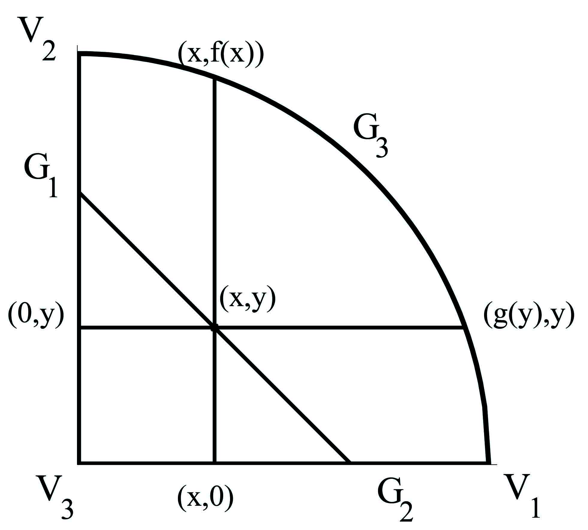
Figure 1: Triangle $\tilde{T}_{h}.$

For $m,n\in\mathbb{N},$ $\beta,b\in\mathbb{R}_{+},$ we consider the following extensions of the Cheney-Sharma operator given in (1):

$$(Q_{m}^{x}F)(x,y) ={\textstyle\sum\limits_{i=0}^{m}}{q}_{m,i}(x,y)F\left(i\tfrac{g(y)}{m},y\right),$$ (4)

$$(Q_{n}^{y}F)(x,y) ={\textstyle\sum\limits_{j=0}^{n}}{q}_{n,j}(x,y)F\left(x,j\tfrac{f(x)}{n}\right),$$

with

$$q_{m,i}\left(x,y\right) ={\tbinom{m}{i}}\tfrac{\tfrac{x}{g(y)}(\tfrac{x}{g(y)}+i\beta)^{i-1}(1-\tfrac{x}{g(y)})[1-\tfrac{x}{g(y)}+(m-i)\beta]^{m-i-1}}{(1+m\beta)^{m-1}},$$

$$q_{n,j}\left(x,y\right) ={\tbinom{n}{j}}\tfrac{\tfrac{y}{f(x)}(\tfrac{y}{f(x)}+jb)^{j-1}(1-\tfrac{y}{f(x)})[1-\tfrac{y}{f(x)}+(n-j)b]^{n-j-1}}{(1+nb)^{n-1}},$$

where

$$\Delta_{m}^{x}=\left\{\left.i\tfrac{g(y)}{m}\right|\ i=\overline{0,m}\right\}\ \text{and }\Delta_{n}^{y}=\left\{\left.j\tfrac{f(x)}{n}\right|\ j=\overline{0,n}\right\}$$

are uniform partitions of the intervals $[0,g(y)]$ and $[0,f(x)].$

Remark 2

As the Cheney-Sharma operator of second kind interpolates a given function at the endpoints of the interval, we may use the operators $Q_{m}^{x}$ and $Q_{n}^{y}$ as interpolation operators.

Theorem 3

If $F$ is a real-valued function defined on $\widetilde{T}_{h}\$then

1. $Q_{m}^{x}F=F\$on $\Gamma_{1}\cup\Gamma_{3},$

2. $Q_{n}^{y}F=F\$on $\Gamma_{2}\cup\Gamma_{3}.$

Proof. (i) We may write

$$(Q_{m}^{x}F)(x,y)= \tfrac{1}{(1+m\beta)^{m-1}}\left\{(1-\tfrac{x}{g(y)})[1-\tfrac{x}{g(y)}+m\beta]^{m-1}F\left(0,y\right)\right.$$ (5)

$$+\tfrac{x}{g(y)}(1-\tfrac{x}{g(y)}){\textstyle\sum\limits_{i=1}^{m-1}}{\tbinom{m}{i}}(\tfrac{x}{g(y)}+i\beta)^{i-1}$$

$$\cdot[1-\tfrac{x}{g(y)}+(m-i)\beta]^{m-i-1}F\left(i\tfrac{g(y)}{m},y\right)$$

$$\left.+\tfrac{x}{g(y)}(\tfrac{x}{g(y)}+m\beta)^{m-1}F\left(g(y),y\right)\right\}.$$

Considering (5), we may easily prove that

$$(Q_{m}^{x}F)(0,y)=F(0,y),$$

$$(Q_{m}^{x}F)(g(y),y)=F(g(y),y).$$

(ii) Similarly, writing

$$(Q_{n}^{y}F)(x,y)= \tfrac{1}{(1+nb)^{n-1}}\left\{(1-\tfrac{y}{f(x)})[1-\tfrac{y}{f(x)}+nb]^{n-1}F\left(x,0\right)\right.$$

$$+\tfrac{y}{f(x)}(1-\tfrac{y}{f(x)}){\textstyle\sum\limits_{j=1}^{n-1}}{\tbinom{n}{j}}(\tfrac{y}{f(x)}+jb)^{j-1}$$

$$\cdot[1-\tfrac{y}{f(x)}+(n-j)b]^{n-j-1}F\left(x,j\tfrac{f(x)}{n}\right)$$

$$\left.+\tfrac{y}{f(x)}(\tfrac{y}{f(x)}+nb)^{n-1}F\left(x,f(x)\right)\right\},$$

we get that

$$(Q_{n}^{y}F)(x,0)=F(x,0),$$

$$(Q_{n}^{y}F)(x,f(x))=F(x,f(x)).$$

 

Theorem 4

The operators $Q_{m}^{x}$ and $Q_{n}^{y}$ have the following orders of accuracy:

1. $\left(Q_{m}^{x}e_{ij}\right)\left(x,y\right)=x^{i}y^{j},\ \ i=0,1;$ $j\in\mathbb{N};$

2. $\left(Q_{n}^{y}e_{ij}\right)\left(x,y\right)=x^{i}y^{j},\$ $i\in\mathbb{N};$ $j=0,1,$ where $e_{ij}\left(x,y\right)=x^{i}y^{j},\$ $i,j\in\mathbb{N.}$

Proof. (i) We have

$$(Q_{m}^{x}e_{ij})(x,y)=y^{j}{\textstyle\sum\limits_{i=0}^{m}}{q}_{m,i}(x,y)[i\tfrac{g(y)}{m}]^{i},$$

and having the degree of exactness of the univariate Cheney-Sharma operator equal to $1$ (see Remark 1), the result follows.

Property (ii) is proved in the same way.    

We consider the approximation formula

$$F=Q_{m}^{x}F+R_{m}^{x}F,$$

where $R_{m}^{x}F$ denotes the approximation error.

Theorem 5

If $F(\cdot,y)\in C[0,g(y)]$ then we have

$$\big{|}\left(R_{m}^{x}F\right)(x,y)\big{|}\leq(1+\tfrac{1}{\delta}\sqrt{A_{m}-x^{2}})\omega(F(\cdot,y);\delta),\ \ \ \ \forall\delta>0,$$ (6)

where $\omega(F(\cdot,y);\delta)$ is the modulus of continuity and $A_{m}=x(1+m\beta)^{1-m}[S(2,m-2,x+2\beta,1-x)-(m-2)\beta S(2,m-3,x+2\beta,1-x+\beta)],$ with $S$ given in (3).

Proof. By Theorem 4 we have that $\operatorname*{dex}(Q_{m}^{x})=1,$ thus we may apply the following property of linear operators (see, for example, [1]):

$$\big{|}(Q_{m}^{x}F)(x,y)-F(x,y)\big{|}\leq[1+\delta^{-1}\sqrt{(Q_{m}^{x}e_{20})(x,y)-x^{2}}]\omega(F(\cdot,y);\delta),\ \ \forall\delta>0,$$

and taking into account (2), we get (6).    

Theorem 6

If $F(\cdot,y)\in C^{2}[0,g(y)]$ then

$$(R_{m}^{x}F)(x,y)= \tfrac{1}{2}F^{(2,0)}(\xi,y)\{x^{2}-x(1+m\beta)^{1-m}[S(2,m-2,x+2\beta,1-x)$$ (7)

$$-(m-2)\beta S(2,m-3,x+2\beta,1-x+\beta)]\},$$

for $\xi\in[0,g(y)]$ and $\beta>0.$

Proof. Taking into account that $\operatorname*{dex}(Q_{m}^{x})=1,$ by Theorem 4, and applying the Peano’s theorem (see, e.g., [28]), it follows

$$(R_{m}^{x}F)(x,y)=\int_{0}^{g(y)}K_{20}(x,y;s)F^{(2,0)}(s,y)ds,$$

where

$$K_{20}(x,y;s)=(x-s)_{+}-\sum_{i=0}^{m}q_{m,i}(x,y)\big{(}i\tfrac{g(y)}{m}-s\big{)}_{+}.$$

For a given $\nu\in\{1,...,m\}$ one denotes by $K_{20}^{\nu}(x,y;\cdot)$ the restriction of the kernel $K_{20}(x,y;\cdot)$ to the interval $\left[(\nu-1)\frac{g(y)}{m},\nu\frac{g(y)}{m}\right],$ i.e.,

$$K_{20}^{\nu}(x,y;\nu)=(x-s)_{+}-\sum_{i=\nu}^{m}q_{m,i}(x,y)\left(i\tfrac{g(y)}{m}-s\right),$$

whence,

$$K_{20}^{\nu}(x,y;s)=\left\{\begin{array}[c]{ll}x-s-\sum\limits_{i=\nu}^{m}q_{m,i}(x,y)\left(i\frac{g(y)}{m}-s\right),&\ s<x\\[8.53581pt] -\sum\limits_{i=\nu}^{m}q_{m,i}(x,y)\left(i\frac{g(y)}{m}-s\right),&\ s\geq x.\end{array}\right.$$

It follows that $K_{20}^{\nu}(x,y;s)\leq 0,\$for $s\geq x.$

For $s<x$ we have

$$K_{20}^{\nu}(x,y;s)= x-s-\sum_{i=0}^{m}q_{m,i}(x,y)\left[i\tfrac{g(y)}{m}-s\right]$$

$$+\sum_{i=0}^{\nu-1}q_{m,i}(x,y)\left[i\tfrac{g(y)}{m}-s\right].$$

Applying Theorem 4, we get

$$\sum_{i=0}^{m}q_{m,i}(x,y)\left[i\tfrac{g(y)}{m}-s\right] =(Q_{m}^{x}e_{10})(x,y)-s(Q_{m}^{x}e_{00})(x,y)$$

$$=x-s,$$

whence it follows that

$$K_{20}^{\nu}(x,y;s)=\sum_{i=0}^{\nu-1}q_{m,i}(x,y)\left[i\tfrac{g(y)}{m}-s\right]\leq 0.$$

So, $K_{20}^{\nu}(x,y;\cdot)\leq 0,$ for any $\nu\in\{1,...,m\},$ i.e., $K_{20}(x,y;s)\leq 0,$ for $s\in[0,g(y)].$

By the Mean Value Theorem, one obtains

$$(R_{m}^{x}F)(x,y)=F^{(2,0)}(\xi,y)\int_{0}^{g(y)}K_{20}(x,y;s)ds,\ \ \text{for }0\leq\xi\leq g(y),$$

with

$$\int_{0}^{g(y)}K_{20}(x,y;s)ds=\tfrac{1}{2}[x^{2}-(Q_{m}^{x}e_{20})(x,y)],$$

and using (2) we get (7).    

Remark 7

Analogous results with the ones in Theorems 5 and 6 could be obtained for the remainder $R_{n}^{y}F$ of the formula $F=Q_{n}^{y}F+R_{n}^{y}F.$

3 Product operators

Let $P_{mn}^{1}=Q_{m}^{x}Q_{n}^{y},$ respectively, $P_{nm}^{2}=Q_{n}^{y}Q_{m}^{x}$ be the products of the operators $Q_{m}^{x}$ and $Q_{n}^{y}.$

We have

$$\left(P_{mn}^{1}F\right)\left(x,y\right)\!=\!\sum_{i=0}^{m}\sum_{j=0}^{n}q_{m,i}\left(x,y\right)q_{n,j}\left(i\tfrac{g(y)}{m},y\right)F\Big{(}i\tfrac{g(y)}{m},j\tfrac{f(i\tfrac{g(y)}{m})}{n}\Big{)},$$

respectively,

$$\left(P_{nm}^{2}F\right)\left(x,y\right)\!=\!\sum_{i=0}^{m}\sum_{j=0}^{n}q_{m,i}\left(x,j\tfrac{f(x)}{n}\right)q_{n,j}\left(x,y\right)F\Big{(}i\tfrac{g(j\tfrac{f(x)}{n})}{m},j\tfrac{f(x)}{n}\Big{)}.$$

Theorem 8

If $F$ is a real-valued function defined on $\widetilde{T}_{h}$ then

1. $(P_{mn}^{1}F)(V_{i})=F(V_{i}),\ \ \ \ i=1,...,3;$

   $(P_{mn}^{1}F)(\Gamma_{3})=F(\Gamma_{3}),\$

2. $(P_{nm}^{2}F)(V_{i})=F(V_{i}),\ \ \ \ i=1,...,3;$

   $(P_{nm}^{2}F)(\Gamma_{3})=F(\Gamma_{3}),\$

Proof. By a straightforward computation, we get the following properties

$$(P_{mn}^{1}F)(x,0)=(Q_{m}^{x}F)(x,0),$$

$$(P_{mn}^{1}F)(0,y)=(Q_{n}^{y}F)(0,y),$$

$$(P_{mn}^{1}F)(x,f(x))=F(x,f(x)),\ \ \ \ \ x,y\in[0,h]$$

and

$$(P_{nm}^{2}F)(x,0)=(Q_{m}^{x}F)(x,0),$$

$$(P_{nm}^{2}F)(0,y)=(Q_{n}^{y}F)(0,y),$$

$$(P_{nm}^{2}F)(g(y),y)=F(g(y),y),\ \ \ \ \ \ x,y\in[0,h],$$

and, taking into account Theorem 3, they imply (i) and (ii).    

We consider the following approximation formula

$$F=P_{mn}^{1}F+R_{mn}^{{}^{P^{1}}}F,$$

where $R_{mn}^{{}^{P^{1}}}$ is the corresponding remainder operator.

Theorem 9

If $F\in C(\widetilde{T}_{h})$ then

$$\left|(R_{mn}^{P^{1}}F)(x,y)\right|\leq(A_{m}+B_{n}-x^{2}-y^{2}+1)\omega(F;\tfrac{1}{\sqrt{A_{m}-x^{2}}},\tfrac{1}{\sqrt{B_{n}-y^{2}}}),\ \forall(x,y)\in\widetilde{T}_{h},$$ (8)

where

$$A_{m}= x(1+m\beta)^{1-m}[S(2,m-2,x+2\beta,1-x)$$ (9)

$$-(m-2)\beta S(2,m-3,x+2\beta,1-x+\beta)]$$

$$B_{n}= y(1+nb)^{1-n}[S(2,n-2,y+2b,1-y)-(n-2)bS(2,n-3,y+2b,1-y+\beta)]$$

and $\omega(F;\delta_{1},\delta_{2})$, with $\delta_{1}>0,$ $\delta_{2}>0,$ is the bivariate modulus of continuity.

Proof. Using a basic property of the modulus of continuity we have

$$\left|(R_{mn}^{P^{1}}F)(x,y)\right|\leq \bigg{[}\tfrac{1}{\delta_{1}}\sum_{i=0}^{m}\sum_{j=0}^{n}q_{m,i}(x,y)q_{n,j}\left(\tfrac{i}{m}g(y),y\right)\left|x-\tfrac{i}{m}g(y)\right|$$

$$+\tfrac{1}{\delta_{2}}\sum_{i=0}^{m}\sum_{j=0}^{n}q_{m,i}(x,y)q_{n,j}\left(\tfrac{i}{m}g(y),y\right)\left|y-\tfrac{j}{n}f\left(\tfrac{i}{m}g(y)\right)\right|$$

$$+\sum_{i=0}^{m}\sum_{j=0}^{n}q_{m,i}(x,y)q_{n,j}\left(\tfrac{i}{m}g(y),y\right)\bigg{]}\omega(F;\delta_{1},\delta_{2}),\ \ \forall\delta_{1},\delta_{2}>0.$$

Since

$$\sum_{i=0}^{m}\sum_{j=0}^{n}p_{m,i}(x,y)q_{n,j}\left(\tfrac{i}{m}g(y),y\right)\left|x-\tfrac{i}{m}g(y)\right|\leq\sqrt{(Q_{m}^{x}e_{20})(x,y)-x^{2}},$$

$$\sum_{i=0}^{m}\sum_{j=0}^{n}p_{m,i}(x,y)q_{n,j}\left(\tfrac{i}{m}g(y),y\right)\left|y-\tfrac{j}{n}f\big{(}\tfrac{i}{m}g(y)\big{)}\right|\leq\sqrt{(Q_{n}^{y}e_{02})(x,y)-y^{2}},$$

$$\sum_{i=0}^{m}\sum_{j=0}^{n}p_{m,i}(x,y)q_{n,j}\left(\tfrac{i}{m}g(y),y\right)=1,$$

applying (2), we get

$$\left|(R_{mn}^{P^{1}}F)(x,y)\right|\leq\left\{\tfrac{1}{\delta_{1}}[x(1+m\beta)^{1-m}]^{\frac{1}{2}}\right.$$

$$\cdot\left\{[S(2,m-2,x+2\beta,1-x)-(m-2)\beta S(2,m-3,x+2\beta,1-x+\beta)]-x^{2}\right\}^{\frac{1}{2}}$$

$$+\tfrac{1}{\delta_{2}}[y(1+nb)^{1-n}]^{\frac{1}{2}}$$

$$\cdot\left\{[S(2,n-2,y+2b,1-y)-(n-2)bS(2,n-3,y+2b,1-y+\beta)]-y^{2}\right\}^{\frac{1}{2}}$$

$$\left.+1\right\}\omega(F;\delta_{1},\delta_{2}).$$

Denoting

$$A_{m} =x(1+m\beta)^{1-m}[S(2,m-2,x+2\beta,1-x)-(m-2)\beta S(2,m-3,x+2\beta,1-x+\beta)]$$

$$B_{n} =y(1+nb)^{1-n}[S(2,n-2,y+2b,1-y)-(n-2)bS(2,n-3,y+2b,1-y+\beta)]$$

and, taking $\delta_{1}=\frac{1}{\sqrt{A_{m}-x^{2}}}$ and $\delta_{2}=\frac{1}{\sqrt{B_{n}-y^{2}}}$, we get (8).    

4 Boolean sum operators

We consider the Boolean sums of the operators $Q_{m}^{x}$ and $Q_{n}^{y}$,

$$S_{mn}^{1} :=Q_{m}^{x}\oplus Q_{n}^{y}=Q_{m}^{x}+Q_{n}^{y}-Q_{m}^{x}Q_{n}^{y},$$

$$S_{nm}^{2} :=Q_{n}^{y}\oplus Q_{m}^{x}=Q_{n}^{y}+Q_{m}^{x}-Q_{n}^{y}Q_{m}^{x}.$$

Theorem 10

If $F$ is a real-valued function defined on $\widetilde{T}_{h},$ then

$$S_{mn}^{1}F\left|{}_{\partial\widetilde{T}_{h}}=F\right|_{\partial\widetilde{T}_{h}},$$

$$S_{mn}^{2}F\left|{}_{\partial\widetilde{T}_{h}}=F\right|_{\partial\widetilde{T}_{h}}.$$

Proof. We have

$$\left(Q_{m}^{x}Q_{n}^{y}F\right)\left(x,0\right)= \left(Q_{m}^{x}F\right)\left(x,0\right){,}$$

$$\left(Q_{n}^{y}Q_{m}^{x}F\right)\left(0,y\right)= \left(Q_{n}^{y}F\right)\left(0,y\right){,}$$

$$\left(Q_{m}^{x}F\right)\left(x,h-x\right)= \left(Q_{n}^{y}F\right)(x,h-x)$$

$$=(P_{mn}^{1}F)(x,h-x)=(P_{nm}^{2}F)(x,h-x)=F(x,h-x),$$

and, taking into account Theorem 3, the conclusion follows.    

We consider the following approximation formula

$$F=S_{mn}^{1}F+R_{mn}^{{}^{S^{1}}}F,$$

where $R_{mn}^{{}^{S^{1}}}$ is the corresponding remainder operator.

Theorem 11

If $F\in C(\widetilde{T}_{h})$ then

$$\big{|}(R_{mn}^{{}^{S^{1}}}F)(x,y)\big{|}\leq$$ (10)

$$\leq(1+A_{m}-x^{2})\omega(F(\cdot,y);\tfrac{1}{\sqrt{A_{m}-x^{2}}})+(1+B_{n}-y^{2})\omega(F(x,\cdot);\tfrac{1}{\sqrt{B_{n}-y^{2}}})$$

$$+(A_{m}+B_{n}-x^{2}-y^{2}+1)\omega(F;\tfrac{1}{\sqrt{A_{m}-x^{2}}},\tfrac{1}{\sqrt{B_{n}-y^{2}}}),$$

with $A_{m}$ and $B_{n}$ given in (9).

Proof. The identity

$$F-S_{mn}^{1}F=(F-Q_{m}^{x}F)+(F-Q_{n}^{y}F)-(F-P_{mn}^{1}F)$$

implies that

$$\big{|}(R_{mn}^{{}^{S^{1}}}F)(x,y)\big{|}\leq\big{|}(R_{m}^{x}F)(x,y)\big{|}+\big{|}(R_{n}^{y}F)(x,y)\big{|}+\big{|}(R_{mn}^{P^{1}}F)(x,y)\big{|},$$

and, applying Theorems 5 and 9, we get (10).    

5 Numerical examples

We consider the function:

$$\begin{array}[c]{ll}\text{Gentle:}&F(x,y)=\frac{1}{3}\exp[-\tfrac{81}{16}\left((x-0.5)^{2}+(y-0.5)^{2}\right)],\end{array}$$

generally used in the literature, (see, e.g., [27]). In Figure 2 we plot the graphs of $F,$ $Q_{m}^{x}F,$ $Q_{n}^{y}F,$ $P_{mn}^{1}F,$ $S_{mn}^{1}F$, on $\tilde{T}_{h},$ considering $h=1,m=5,$ $n=6$, $\beta=1$ and we can see the good approximation properties.

$F$

$Q_{m}^{x}F$

$Q_{n}^{y}F$

$P_{mn}^{1}F$

$S_{mn}^{1}F$

Figure 2: The Cheney-Sharma approximants for $\tilde{T}_{h}.$

References

• [1] O. Agratini, Approximation by linear operators, Cluj University Press, 2000.
• [2] R. E. Barnhill, Blending function interpolation: a survey and some new results, Numerishe Methoden der Approximationstheorie, (Eds. L. Collatz et al., Vol. 30, Birkhauser-Verlag, Basel, 1976), pp. 43-89.
• [3] R. E. Barnhill, Representation and approximation of surfaces, Mathematical Software III, (Ed. J.R. Rice, Academic Press, New-York, 1977), pp. 68-119.
• [4] R. E. Barnhill, G. Birkhoff, W. J. Gordon, Smooth interpolation in triangles, J. Approx. Theory, 8, pp. 114–128 (1973).
• [5] R. E. Barnhill, J. A. Gregory, Compatible smooth interpolation in triangles, J. Approx. Theory, 15, pp. 214-225 (1975).
• [6] R. E. Barnhill, J. A. Gregory, Sard kernels theorems on triangular domains with applications to finite element error bounds, Numer. Math., 25, pp. 215-229 (1976).
• [7] C. Bernardi, Optimal finite-element interpolation on curved domains, SIAM J. Numer. Anal., 26, no. 5, pp. 1212-1240 (1989).
• [8] P. Blaga, T. Cătinaş, G. Coman, Bernstein-type operators on tetrahedrons, Studia Univ. Babes-Bolyai, Mathematica, 54, no. 4, pp. 3-19 (2009).
• [9] P. Blaga, T. Cătinaş, G. Coman, Bernstein-type operators on a square with one and two curved sides, Stud. Univ. Babeş-Bolyai Math., 55, no. 3, pp. 51-67 (2010).
• [10] P. Blaga, T. Cătinaş, G. Coman, Bernstein-type operators on triangle with all curved sides, Appl. Math. Comput., 218, pp. 3072–3082 (2011).
• [11] P. Blaga, T. Cătinaş, G. Coman, Bernstein-type operators on triangle with one curved side, Mediterr. J. Math., 9, No. 4, pp. 843-855 (2012).
• [12] K. Böhmer, G. Coman, Blending interpolation schemes on triangle with error bounds, Lecture Notes in Mathematics, 571, Springer Verlag, Berlin, Heidelberg, New York, 1977, pp. 14–37.
• [13] T. Cătinaş, G. Coman, Some interpolation operators on a simplex domain, Stud. Univ. Babeş–Bolyai Math., 52, no. 3, 25–34 (2007).
• [14] T. Cătinaş, Extension of some particular interpolation operators to a triangle with one curved side, Appl. Math. Comput., 315, pp. 286–297 (2017).
• [15] T. Cătinaş, P. Blaga, G. Coman, G., Surfaces generation by blending interpolation on a triangle with one curved side, Results Math., 64, nos. 3-4, pp. 343-355 (2013).
• [16] E.W. Cheney, A. Sharma, On a generalization of Bernstein polynomials, Riv. Mat. Univ. Parma, 5, 77-84 (1964).
• [17] G. Coman, T. Cătinaş, Interpolation operators on a tetrahedron with three curved sides, Calcolo, 47, no. 2, pp. 113-128 (2010).
• [18] G. Coman, T. Cătinaş, Interpolation operators on a triangle with one curved side, BIT Numer. Math., 50, no. 2, pp. 243-267 (2010).
• [19] G. Coman, I. Gânscă, Some practical application of blending approximation II, Itinerant Seminar on Functional Equations, Approximation and Convexity, Cluj-Napoca, pp. 75-82 (1986).
• [20] G. Coman, I. Gânscă, L. Ţâmbulea, Some new roof-surfaces generated by blending interpolation technique, Stud. Univ. Babeş-Bolyai Math., 36, 1, pp. 119-130 (1991).
• [21] W. J. Gordon, Ch. Hall, Transfinite element methods: blending-function interpolation over arbitrary curved element domains, Numer. Math., 21, pp. 109-129 (1973).
• [22] W. J. Gordon, J.A. Wixom, Pseudo-harmonic interpolation on convex domains, SIAM J. Numer. Anal., 11, No 5, pp. 909-933 (1974).
• [23] J. A. Marshall, R. McLeod, Curved elements in the finite element method, Conference on Numer. Sol. Diff. Eq., Lectures Notes in Math., 363, Springer Verlag, pp. 89-104 (1974).
• [24] J. A. Marshall, A. R. Mitchell, An exact boundary tehnique for improved accuracy in the finite element method, J. Inst. Maths. Applics., 12, pp. 355-362 (1973).
• [25] J. A. Marshall, A. R. Mitchell, Blending interpolants in the finite element method, Inter. J. Numer. Meth. Engineering, 12, pp. 77-83 (1978).
• [26] A. R. Mitchell, R. McLeod, Curved elements in the finite element method, Conference on Numer. Sol.Diff. Eq., Lectures Notes in Mathematics, 363, pp. 89-104 (1974).
• [27] R. J. Renka, A. K. Cline, A triangle-based $C^{1}$ interpolation method, Rocky Mountain J. Math. 14, pp. 223–237 (1984).
• [28] A. Sard, Linear Approximation, American Mathematical Society, Providence, Rhode Island, 1963.
• [29] L. L. Schumaker, Fitting surfaces to scattered data, Approximation Theory II, (Eds. G. G. Lorentz, C. K. Chui, L. L. Schumaker, Academic Press, 1976), pp. 203–268.
• [30] D. D. Stancu, C. Cişmaşiu, On an approximating linear positive operator of Cheney-Sharma, Rev. Anal. Numer. Theor. Approx., 26, pp. 221-227 (1997).
• [31] M. Zlamal, Curved elements in the finite element method I, SIAM J. Numer. Anal., 10, pp. 229-240 (1973).