Dirac points merging and wandering in a model Chern insulator

Abstract

We present a model for a Chern insulator on the square lattice with complex first and second neighbor hoppings and a sublattice potential which displays an unexpectedly rich physics. Similarly to the celebrated Haldane model, the proposed Chern insulator has two topologically non-trivial phases with Chern numbers $\pm 1$. As a distinctive feature of the present model, phase transitions are associated to Dirac points that can move, merge and split in momentum space, at odds with Haldane’s Chern insulator where Dirac points are bound to the corners of the hexagonal Brillouin zone. Additionally, the obtained phase diagram reveals a peculiar phase transition line between two distinct topological phases, in contrast to the Haldane model where such transition is reduced to a point with zero sublattice potential. The model is amenable to be simulated in optical lattices, facilitating the study of phase transitions between two distinct topological phases and the experimental analysis of Dirac points merging and wandering.

I Introduction

The study of topological phases in electronic systems, particularly topological insulators, have become an area of vast interest in condensed matter physics (Hasan and Kane, 2010; Qi and Zhang, 2011; with Taylor L. Hughes, 2013). Arguably, the first experimenal realization of a topological electron system is associated with the discovery of the quantum Hall effect by von Klitzing (Klitzing et al., 1980) almost fourty years ago. This phenomenon takes place in two-dimensional systems at high magnetic fields, when a quantized Hall conductivity and dissipationless surface conducting states appear. High magnetic fields are not easy to realize, which motivates the interest for an effect with the same transport properties under a zero applied magnetic field – the quantum anomalous Hall effect (Nagaosa et al., 2010).

Both quantum Hall and quantum anomalous Hall systems are two-dimensional insulators with broken time-reversal symmetry. Their topological character is associated with a topological invariant called first Chern number ($C$), which is equal to the Hall conductivity in units of $e^{2}/h$ (Xiao et al., 2010). Different Chern numbers describe different topological phases of matter, while $C=0$ corresponds to the normal insulating phase. In modern language this systems are known as Chern insulators (with Taylor L. Hughes, 2013).

Figure 1: (a) Phase diagram of the Haldane model. (b) Phase diagram of the model proposed in Eq. 2.

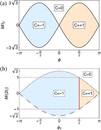
The first theoretical realization of the quantum anomalous Hall effect is due to Haldane (Haldane, 1988). He proposed a Chern insulator toy model considering a honeycomb lattice with two different types of atoms subjected to a sublattice potential $\pm M$ and with second nearest neighbor complex hoppings of the type $t_{2}e^{\pm i\phi}$. These hoppings were responsible for breaking time reversal symmetry and are the effect of a local magnetic flux density built in such a way that its total flux in the unit cell, and therefore in the whole system, is zero. Depending on the values chosen for the parameters of the Haldane model – $M$ and $\phi$ – it is possible to obtain a trivial insulating phase ($C=0$) or topological phases with $C=\pm 1$, as can be seen in fig. 1(a) where we show the phase diagram of the Haldane model, reproduced here for clarity and comparison. Believed to be of unlikely realization in a solid state system, this model settled ground to the discovery of time reversal invariant topological insulators (Kane and Mele, 2005; Bernevig and Zhang, 2006; Bernevig et al., 2006; Konig et al., 2007), which fuelled the field in the last decade (Chiu et al., 2016). The observation of the quantum anomalous Hall effect was acheived in a magnetic topological insulator (Chang et al., 2013). This was followed by an experimental realization of the pioneer Haldane model using cold atoms trapped in optical lattices (Jotzu et al., 2014), opening the door to study the effect of interactions (Gonçalves et al., 2018b) and disorder (Gonçalves et al., 2018a; Castro et al., 2015, 2016) in Chern insulators experimentally in a controlled way.

In the presence of multiple energy bands and translational invariance, a topological phase transition is associated to a gap closing at some band crossing point(s) in the reciprocal space (Haldane, 2004; Sun and Fradkin, 2008). If the energy dispersion relation near these points is linear in the reciprocal space vector $\bm{k}$, they are called Dirac points (with Taylor L. Hughes, 2013). Since Dirac points are monopoles of Berry curvature (Haldane, 2004), they arise naturally in Chern insulators at the boundary between phases with different Chern number. In the Haldane model, as recognized in the seminal paper (Haldane, 1988), there is a single Dirac point along the full phase transition line shown in fig. 1(a), except at the point $M=0$, $\phi=0$, where there are two Dirac points – the case of graphene. Either one or two, Dirac points in the Haldane model are bound to the corners of the hexagonal Brillouin zone and they do not move by changing the parameters $M$ and $\phi$ of the model.

Under certain conditions, Dirac points can move, merge and split in $\bm{k}$-space for continuous variations of the Hamiltonian parameters. This can be achieved, for example, by considering models with asymmetric changes in the hopping parameters (Montambaux et al., 2009a, b; Lim et al., 2012; Hasegawa and Kishigi, 2012; Sticlet and Piéchon, 2013). In graphene, hopping changes may be induced by applying strain (Pereira et al., 2009; Vozmediano et al., 2010), but the high strain values required strongly limit the effect. To circumvent this limitation, moving and merging Dirac points have been proposed in ac-driven graphene (Delplace et al., 2013), patterned graphene (Dvorak and Wu, 2015), and artificial graphene (Feilhauer et al., 2015). They have also been proposed in honeycomb optical lattices (Wunsch et al., 2008; Sriluckshmy et al., 2014) and square optical lattices (Hou, 2014), which seem to be even better platforms. Indeed, the ability to create, move and merge Dirac points (Tarruell et al., 2012; Tarnowski et al., 2017), has been recently demonstrated using honeycomb optical lattices. Possible applications of merging Dirac points range from valleytronics (Ang et al., 2017) to plasmonics (Pyatkovskiy and Chakraborty, 2016). Interesting effects due to electron-electron interactions (Dóra et al., 2013; Wang and Fu, 2013) and disorder have also been proposed (Carpentier et al., 2013).

Here we propose new model for a Chern insulator realized on the square lattice, with a richer phase diagram than the Haldane model, as shown in fig. 1(b). Two interesting properties stand out: (i) a topological transition between $C=\pm 1$ phases exists for a finite staggered potencial range $-1<M<+1$, as depicted by the vertical red line in fig. 1(b), while in the Haldane model such transition is reduced to the point $M=0$, $\phi=0$; (ii) up to four Dirac points are found at the phase transition lines, which are allowed to wander, merge, and split in reciprocal space as a function of the model parameters $M$ and $\phi_{3}$ (to be explained below), while in the Haldane model they are bound to fixed momenta. The model can be simulated using a square optical lattice, enabling the simultaneous analysis of Chern insulating phases and their phase transitions, as well as the movement, merging and splitting of Dirac points. Semi-Dirac points are also realized for some merging conditions.

II Model and methods

II.1 A simple square lattice model

We present here a toy model composed by a lattice with two interpenetrating square lattices of atoms A and B, as shown in fig. 2. This model considers complex hoppings between first and second neighbors, respectively of the type $t_{1}e^{i\varphi_{1}^{\alpha}}$ and $t_{2}e^{i\varphi_{2}^{\beta}}$, with $\alpha$ and $\beta$ being respectively the four indexes of the first and second neighbors. The phases $\varphi_{1}^{\alpha}$ and $\varphi_{2}^{\beta}$ were imposed in such a way that the total flux in the unit cell, $\Phi_{T}$, is null. Designating $\phi_{i}$ as the flux over each of the four triangles composing the unit cell, as represented in fig. 2, we impose $\Phi_{T}=\sum_{i=1}^{4}\phi_{i}=0$. This condition does not univocally fix the phases, and we indicate our choice for the phases $\varphi_{1}^{\alpha}$ and $\varphi_{2}^{\beta}$ explicitly in Fig. 2.

Figure 2: Representation of the lattice used for the toy model. The red and blue atoms correspond respectively to different atoms of types A and B. The complex hopping phases are given for each hopping and the flow of the corresponding flux is represented by the arrows.

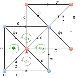
The free parameters of our model were chosen to be the phase $\phi_{3}$ (and not $\phi$ to clearly distinguish from the fluxes in Haldane model) represented in fig. 2 and a sublattice potential $M$: $+M$ for sites A and $-M$ for sites B. For the present choice, the remaining fluxes are given by,

$$\phi_{1}= -\pi/2$$

$$\phi_{2}= \pi$$

$$\phi_{4}= -\pi/2-\phi_{3}\,.$$ (1)

The considered fluxes are asymmetric in that they explicitly break the $C_{4}$ symmetry of the original lattice.

The Hamiltonian of the present model is easily written in direct space using second quantization and the field operators $c_{\boldsymbol{r}}^{\dagger}$, where $c_{\boldsymbol{r}}^{\dagger}=(a_{\boldsymbol{r}}^{\dagger},b_{\boldsymbol{r}}^{\dagger})$ is the creation operator in the sublattice pseudospin space ($a,b$ denoting the A and B sublattices, respectively) acting on the unit cell at position $\boldsymbol{r}$. Taking into account translational invariance and introducing the Bloch basis, $c_{\bm{r}}^{\dagger}=\frac{1}{\sqrt{N}}\sum_{\bm{{k}}}e^{-i\bm{{k.\bm{{r}}}}}c_{\bm{{k}}}^{\dagger}$, we can write the Hamiltonian of our toy model in the reciprocal space as $H=\sum_{\bm{k}}\Psi_{\bm{k}}^{\dagger}H(\bm{k})\Psi_{\bm{k}}$, where $\Psi_{\bm{k}}^{\dagger}=(a_{\bm{k}}^{\dagger},b_{\bm{k}}^{\dagger})$ and

$$H(\bm{k})=\begin{bmatrix}g(\bm{k})+M&f(\bm{k})\\ f^{*}(\bm{k})&-g(\bm{k})-M\end{bmatrix}\,,$$ (2)

with

$$g(\bm{k})= 2t_{2}[cos(\bm{k}.\bm{a_{1}})-cos(\bm{k}.\bm{a_{2}})]\,,$$ (3)

$$f(\bm{k})= t_{1}[-i+e^{i\bm{k}.\bm{a_{1}}}+e^{-i\phi_{3}}e^{i\bm{k}.\bm{a_{2}}}+e^{i\bm{k}.(\bm{a_{1}}+\bm{a_{2}})}]\,,$$ (4)

and the primitive unit vectors $\bm{a_{1}}=a(1,0)$ and $\bm{a_{2}}=a(0,1)$, written in terms of the lattice constant $a$.

It is useful to write the hamiltonian in terms of the Pauli matrices. In units where the lattice constant $a=1$, it becomes

$$H(\bm{k})=\bm{h(\bm{k})}.\bm{\sigma}\,,$$ (5)

with the vector $\boldsymbol{h}$ given by

$$h_{x}(\bm{k})= t_{1}[\cos k_{x}+\cos(-\phi_{3}+k_{y})+\cos(k_{x}+k_{y})]$$

$$h_{y}(\bm{k})= t_{1}[1-\sin k_{x}-\sin(-\phi_{3}+k_{y})-\sin(k_{x}+k_{y})]$$

$$h_{z}(\bm{k})= 2t_{2}(\cos k_{x}-\cos k_{y})+M\,,$$ (6)

and $\boldsymbol{\sigma}=(\sigma_{x},\sigma_{y},\sigma_{z})$ is the vector of Pauli matrices. From eq. (5), the band spectrum is simply obtained as $\epsilon(\bm{k})=\pm|\bm{h}|$. As shown below, analytic expression for band crossing points can be obtained by solving $\epsilon(\bm{k})=0$.

When the Hamiltonian is in the form of eq. (5), the Chern number $C$ can be calculated using the following expression (Xiao et al., 2010),

$$C=\frac{1}{4\pi}\int_{\mathrm{BZ}}\frac{\partial\bm{h}}{\partial k_{x}}\times\frac{\partial\bm{h}}{\partial k_{y}}\cdot\frac{\bm{h}}{|h|^{3}}\,dk_{x}dk_{y}\,,$$ (7)

where the integration is performed over the Brillouin zone (BZ): $k_{x},k_{y}\in[-\pi,\pi]$.

II.2 Low energy, continuum approximation

In the presence of a topological phase transition, the spectral gap existing in the insulating phase closes at some band crossing points. These gap closing points are responsible for the change in the Chern number between the phases. Near these points the band crossing is generally linear (Haldane, 2004), and we are able to linearize the Hamiltonian in eq. (5) provided we are close enough to the phase transition.

Let us assume that a band crossing point exists at point P in the BZ associated to a given phase transition in the phase diagram. After linearization around P, assuming the parameters are such that the system is close to the phase transition, we may approximate eq. (5) by

$$H^{\mathrm{P}}(\bm{\kappa})=\kappa_{\alpha}\mathcal{G}_{\alpha\beta}^{\mathrm{P}}\sigma_{\beta}\,,$$ (8)

where $\bm{\kappa}\equiv(\kappa_{x},\kappa_{y})=\bm{k}-\bm{k}_{\mathrm{P}}$ is the small momentum relative to $\boldsymbol{k}_{\mathrm{P}}$, with $\boldsymbol{k}_{\mathrm{P}}$ the momentum associated to the band crossing point P. In eq. (8), summation over repeated indeces is assumed, with $\kappa_{z}=1$, and the matrix $\mathcal{G}^{\mathrm{P}}$ is the matrix obtained by expanding the Hamiltonian in eq. (5) around a given band crossing point P. Due to the linear form of the approximate Hamiltonian in eq. (8), these gap closing points are called Dirac points.

The contribution of the Dirac point P to the Chern number, $C_{\mathrm{P}}$, is obtained using eq. (7) and (8),

$$C_{\mathrm{P}}=\frac{1}{2}\text{sgn}[\det(\mathcal{G}^{\mathrm{P}})]\,.$$ (9)

If we obtain $C_{\mathrm{P}}$ in two distinct phases close to the phase transition, we may then compute the difference between the two results, $\Delta C_{\mathrm{P}}$. Since the high energy contributions cancel, we obtain the total contribution of this Dirac point to the change in Chern number at the phase transition (Lovesey, 2014). We use $\Delta C_{\mathrm{P}}$ to further characterize the phase diagram of the proposed Chern insulator.

III Results

III.1 Phase diagram

The obtained phase diagram is shown in fig. 1(b). It was obtained through eq. (7) and confirmed numerically with the Fukui method (Fukui et al., 2005).

The $C=0$ phase corresponds to a normal insulator. The energy gap closes at the dashed and dotted curves which correspond to phase transition lines between a trivial and a topological phase. There are two topological phases with $C=\pm 1$ corresponding to the filled regions in fig. 1(b). They are separated by a vertical phase transition line existing at $\phi_{3}=\pi/2$. The equations for the dotted, dashed, and solid phase transition lines shown in fig. 1(b) are

$$\begin{cases}M(\phi_{3})=\pm 2\sqrt{2}t_{2}\cos(\phi_{3}/2)&\text{{dotted(+)/dashed(-)}}\\ \phi_{3}=\pi/2\cap\Big{|}\frac{M}{2t_{2}}\Big{|}<1&\text{{solid\,(vertical)}}\,.\end{cases}$$ (10)

There is yet another line not depicted in fig. 1(b), correponding to $\phi=\pi/2$ and $-4t_{2}<M<-2t_{2}$, which does not correspond to any phase transition but for which the energy spectrum is gapless.

Figure 3: Motion of the Dirac points along the $\phi_{3}=\pi/2$ phase transition line: (a) $M>2t_{2}$, (b) $M=2t_{2}$, (c) $M=t_{2}$, (d) $M=0$, (e) $M=-t_{2}$, (f) $M=-2t_{2}$.

III.2 Wandering of Dirac points and its consequences

We have analyzed the evolution of the number of Dirac points, as well as their position in the BZ, along the phase transition lines shown in fig. 1(b). We have verified that the position of the Dirac points changes along the transition lines. Furthermore, the number of band crossing points is not conserved. In this section we provide a detailed analysis of this behavior.

III.2.1 Single band crossing point

The dotted curve in fig. 1(b) is associated with a single band crossing point everywhere, except at $\phi_{3}=\pm\pi$ where there are two Dirac points. The same applies to the dashed curve, except at $\phi_{3}=\pi/2$, where it also has two band crossing points. For for $\phi_{3}\neq\{\pm\pi,\pi/2\}$, the position of the single Dirac point along these curves is given, for the dotted curve, by

$$\begin{cases}(k_{x},k_{y})=(x_{M_{+}},y_{M_{+}})&\phi_{3}<0\\ (k_{x},k_{y})=(x_{M_{-}},y_{M_{-}})&\phi_{3}>0\end{cases}\,,$$ (11)

and for the dashed curve, by

$$\begin{cases}(k_{x},k_{y})=(x_{M_{-}},y_{M_{-}})&\phi_{3}<0\\ (k_{x},k_{y})=(x_{M_{+}},y_{M_{+}})&\phi_{3}>0\end{cases}\,,$$ (12)

where

$$\begin{cases}x_{M_{\pm}}=\pm 2\text{arctan}\left[\frac{M+2t_{2}}{\sqrt{8t_{2}^{2}-M^{2}}\pm 2t_{2}}\right]\\ y_{M_{\pm}}=2\text{arctan}\left[\frac{\sqrt{8t_{2}^{2}-M^{2}}\mp M}{\sqrt{8t_{2}^{2}-M^{2}}\pm(M+4t_{2})}\right]\end{cases}\,.$$ (13)

III.2.2 Multiple band crossing points

At $\phi_{3}=\pm\pi$, we have two Dirac points at $(k_{x},k_{y})=(-3\pi/4,-3\pi/4)$ and $(k_{x},k_{y})=(\pi/4,\pi/4)$. For $\phi_{3}=\pi/2$, the phase transition line is very rich in terms of band crossing points as their number ranges between 1 and 4 due to merging and splitting of Dirac points. This case is analyzed in the following.

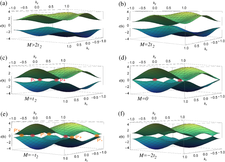
Let us fix $\phi_{3}=\pi/2$. As long as $M>2t_{2}$, we are not yet at the phase transition line and there is a gap in the energy spectrum corresponding to a trivial insulator [fig. 3(a)]. This gap closes for $M=2t_{2}$, at a single band crossing point, $(k_{x},k_{y})=(\pi/2,0)$, [fig. 3(b)]. This band crossing point is not a conventional Dirac point, as the energy spectrum is quadratic in the $k_{y}$ direction and linear in $k_{x}$ – which is called a semi-Dirac point (Montambaux et al., 2018). This is known to be a consequence of the merging of two Dirac points (Montambaux et al., 2009b, a; Banerjee et al., 2009; Li et al., 2015; Adroguer et al., 2016), in this case in the $k_{y}$ direction. Indeed, topological phase transitions accompained with higher order band crossings, for example quadratic band crossings, exist and can be interpreted as the merging of two or more Dirac points (Sun et al., 2009).

Slightly reducing $M$, still with fixed $\phi_{3}=\pi/2$, we observe that the semi-Dirac point splits in the above mentioned two Dirac points in the $k_{y}$ direction [fig. 3(c)], which we call $\mathrm{P}_{+}$ and $\mathrm{P}_{-}$. These points move away from each other in the $k_{y}$ direction, untill they reach the boundaries of the BZ for $M=-2t_{2}$ [fig. 3(f)], where they again merge. Their coordinates for $-2t_{2}<M<2t_{2}$ are given by

$$P_{\pm}=\left\{\frac{\pi}{2},\pm\text{$\arccos$}\left(\frac{M}{2t_{2}}\right)\right\}\,.$$ (14)

For $M=0$ [fig. 3(d)], a new band crossing point shows up at the boundaries of the BZ, $(k_{x},k_{y})=(\pm\pi,\pm\pi)$. This point is also a semi-Dirac point, being quadratic in the $k_{x}$ direction. For $-2t_{2}<M<0$ [fig. 3(e)], this single point splits in two in the $k_{x}$ direction, which we call $P^{\prime}_{+}$ and $P^{\prime}_{-}$, with coordinates given by

$$P^{\prime}_{\pm}=\left\{\pi,\pm\text{arccos}\left(-\frac{M}{2t_{2}}-1\right)\right\}\,.$$ (15)

An important detail not shown in the figures is that these points exist for $-4t_{2}<M<0$, and therefore survive outside the boundaries of the $\phi_{3}=\pi/2$ phase transition line. They give rise to the gapless spectrum associated with the extension of the vertical transition line in fig. 1(b), mentioned in section III.1.

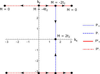
A global overview of the motion, merging and splitting of the Dirac points for the $\phi=\pi/2$ gapless region of the phase diagram ($-4t_{2}<M<2t_{2}$) is given in figure 4.

Figure 4: Overview of the motion, merging and splitting of the Dirac points in the BZ for $\phi_{3}=\pi/2$ and $-4t_{2}<M<2t_{2}$ [along the vertical line in Fig. 1(b)]. All four Dirac points existing in this region, $P_{\pm}$ and $P^{\prime}_{\pm}$ [eq. (14) and (15)], are depicted in the figure with the corresponding motion lines given in the legend. The arrows point to regions of higher $M$ and the dots describe the merging or splitting of Dirac points.

III.2.3 Contribution to the topological invariant

Based on the methods from section II.2, we computed the contributions of Dirac points to the Chern number for the different phase transition curves. For curves associated to a single Dirac point [dashed and dotted in fig. 1(b)], its contribution was confirmed to be trivially $\Delta C=1$.

For the $\phi_{3}=\pi/2$ phase transition line the contributions are as follows. By expanding the Hamiltonian in eq. (5) around $P_{+}$, the contribution to the Chern number obtained from eq. (9) is

$$C_{P_{+}}=\begin{cases}-1/2&\phi_{3}\lesssim\pi/2\\ 1/2&\phi_{3}\gtrsim\pi/2\end{cases}\,.$$ (16)

This meas that $P_{+}$ contributes with $\Delta C_{P_{+}}=1$ for the change in the Chern number. Doing the same for $P_{-}$, we verified that this point had exactly the same contribution. Therefore, $P_{+}$ and $P_{-}$ contribute to a total change of $\Delta C=2$ between the topological phases. For the points $P^{\prime}_{+}$ and $P^{\prime}_{-}$, we obtained that for all their domain of existence

$$C_{P^{\prime}_{+}}=-C_{P^{\prime}_{-}}=\begin{cases}1/2&\phi_{3}\lesssim\pi/2\\ -1/2&\phi_{3}\gtrsim\pi/2\end{cases}\,,$$ (17)

thus giving canceling contributions. We then conclude that $P_{+}$ and $P_{-}$ are the points responsible for the change from $C=-1$ to $C=1$ between topological phases. It thus makes sense that $P_{+}$ and $P_{-}$ exist for $-2t_{2}<M<2t_{2}$, while and the additional points $P^{\prime}_{+}$ and $P^{\prime}_{-}$ exist for $-4t_{2}<M<0$. If the latter were to have any net contribution for the topological transition, we would have a phase transition for $-4t_{2}<M<2t_{2}$ which is not the case.

IV Conclusions

We have put forward a new model for a Chern insulator which is characterized by a richer phase diagram than the celebrated Haldane Chern insulator. An interesting new result regarding the obtained phase diagram is the appearance of a phase transition line between topological phases in the $(M,\phi_{3})$ parameter space. This implies a transition between non-trivial phases for non-zero sublattice potential. This phenomenon does not occur for the Haldane model in which the transition between $C=\pm 1$ phases occurs only for $M=0$ [compare fig. 1(a) with 1(b)].

Another striking characteristic of the proposed Chern insulator is that Dirac points at the phase transition lines can move, merge, and split in reciprocal space, while in the Haldane model they are bound to fixed momenta. Of particular relevance is the behavior of Dirac points for the vertical transition line in fig. 1(b), when $\phi_{3}=\pi/2$. There, up to four Dirac points are found, which move as $M$ is changed, merging in pairs as semi-Dirac points, with subsequent annihilation or splitting. Of the four Dirac points found, only two contribute to the change $\Delta C=2$ in Chern number across the phase transition, where $C=+1$ on one side of the transition line and $C=-1$ on the other. The phase transition exists as long as both points are separated and ceases to exist when they merge and a trivial insulating gap is opened.

The model here proposed extends the physics of moving and merging Dirac points, studied previously in models with tunable hopping values (Wunsch et al., 2008; Montambaux et al., 2009b; Hou, 2014), to the realm of Chern insulators where only hopping phases ($\phi_{3}$ in the present case), and not their absolute values, have to be changed. It also enables the study of semi-Dirac points (Li et al., 2015) within the same set up where Chern insulating phases are realized.

The realization of the Haldane Chern insulator (Jotzu et al., 2014), as well as the ability to create, move and merge Dirac points (Tarruell et al., 2012; Tarnowski et al., 2017), has been recently demonstrated using ultracold atoms in an optical lattice. In Refs. (Jotzu et al., 2014) and (Tarruell et al., 2012; Tarnowski et al., 2017), a challenging honeycomb lattice to trap fermionic atoms had to be realized using interfering laser beams. Within the present model, a much simpler square lattice is required, thus facilitating the study of Chen insulating properties and Dirac points merging and wandering, which can be done simultaneously within the same setting. It would also be interesting to study the effect of interactions in such a rich playground (Cocks et al., 2012).