Phase behaviour in ionic solutions: restricted primitive model of ionic liquid in explicit neutral solvent

Abstract

We study fluid-fluid equilibrium in the simplest model of ionic solutions where the solvent is explicitly included, i.e., a binary mixture consisting of a restricted primitive model (RPM) and neutral hard-spheres (RPM-HS mixture). First, using the collective variable method we find free energy, pressure and partial chemical potentials in the random phase approximation (RPA) for a rather general model that takes into consideration solvent-solvent and solvent-ion interactions beyond the hard core. In the special case of a RPM-HS mixture, we consider two regularizations of the Coulomb potential inside the hard core, i.e., the Weeks-Chandler-Andersen (WCA) regularization leading to the WCA approximation and the optimized regularization giving the optimized RPA (ORPA) or the mean spherical approximation (MSA). Furthermore, we calculate the phase coexistence using the associative mean spherical approximation (AMSA). In general, the three approximations produce qualitatively similar phase diagrams of the RPM-HS mixture, i.e., a fluid-fluid coexistence envelope with an upper critical solution point, a shift of the coexistence region towards higher total number densities and higher solvent concentrations with increasing pressure, and a small increase of the critical temperature with an increase of pressure. As for a pure RPM, the AMSA leads to the best agreement with the available simulation data when the association constant proposed by Olaussen and Stell is used. We also discuss the peculiarities of the phase diagrams in the WCA approximation.

1 Introduction

The liquid-liquid phase equilibrium in electrolyte solutions and room temperature ionic liquids (ILs) represents one of the most important problems in physical chemistry and chemical engineering. In particular, the understanding of phase behaviour is essential in extraction, purification and many other industrial applications.

Most theoretical and computer simulation studies of ionic systems are based on the restricted primitive model (RPM), i.e., an equimolar mixture of equisized charged hard spheres immersed in a structureless dielectric continuum. Theoretical studies of the RPM predict the vapour-liquid-like phase transition at low reduced temperatures and at low reduced densities [1, 2, 3, 4]. Reliable estimates of the location of the critical point have been obtained by using mixed-field finite-size (MFFS) scaling methods of computer simulations [5, 6]. In accordance with the prediction of the RPM, the liquid-liquid critical points of ILs in non-polar solvents are located at low temperatures and at low concentrations when the critical parameters are expressed in terms of the RPM variables [7, 8, 9, 10]. However, systematic deviations of the reduced critical temperature with the dielectric constant of a solvent indicate the limitations of the analogy of a liquid-liquid transition in ionic solutions compared to the vapour-liquid transition of the RPM [9, 10, 11]. Modified versions of the RPM that take into account the charge or/and size asymmetry, the so-called primitive models (PM), were also studied theoretically [12, 13, 14, 15, 16, 17, 18, 19, 20] and by Monte Carlo (MC) simulations [21, 22, 23, 24, 25, 26, 27, 28, 29]. A comprehensive overview of the phase diagrams of ILs in a variety of polar and non-polar solvents and the comparison of these diagrams with the results of model systems, in particular, the PM and the RPM, show that more complex models should be used to properly describe these systems [10, 11]. In this connection, models that take the structure of solvents into consideration are of particular interest.

In the simplest model that takes into account a discrete structure of the solvent, the ions are modelled by charged hard spheres while the solvent molecules are neutral hard spheres. The polar nature of the solvent is represented implicitly by a continuum background with a dielectric constant. This model is often called a solvent primitive model or the SPM (see [30] and references therein). However, the above-mentioned abbreviation was also used for another model, the so-called special primitive model, that is the PM with the same ion diameter but with different valences (see e.g. [3]). To avoid misunderstandings, thereafter we refer to a binary mixture of the PM and the neutral hard spheres as the PM-HS mixture (or the RPM-HS mixture for the equisized monovalent PM). The phase behaviour of the RPM-HS mixture was theoretically studied by using the mean-spherical approximation (MSA) [31] and the pairing MSA (PMSA) [32]. For the pure RPM fluid, the PMSA theory leads only to a slight decrease of the critical temperature when compared to the MSA results but it noticeably improves the MSA critical density [33]. As it was shown in [31, 32], the critical temperature of the RPM-HS mixture expressed in the RPM reduced variables is a bit higher than for the RPM. To the best of our knowledge, only a few MC simulation results of phase coexistence in the RPM-HS fluid have been reported [30, 34]. They were obtained without the use of the MFFS scaling.

The purpose of this paper is to study the phase behaviour of ionic models that take into account the presence of the solvent explicitly. To this end, we use two theoretical approaches, i.e., the theory that uses the collective variable (CV) method [35, 36] and the associative mean spherical approximation (AMSA) that exploits the concept of ion association [37, 38, 39]. For the RPM-HS mixture, the AMSA theory reduces to the MSA when the association between ions is neglected. On the other hand, the Helmholtz free energy in the MSA can be obtained within the framework of the CV theory from the random phase approximation (RPA) using an optimized regularization of the Coulomb potential inside the hard core [40].

By applying the CV theory, we start with a general model where the interaction potentials between the two solvent particles and between the ion and the solvent particle include a short-range attraction/repulsion in addition to a hard-core repulsion. Moreover, the positive and negative ions and the ions and the solvent particles can differ in size. For this model, free energy in the RPA is obtained. Here, we address the phase diagrams of an equisized RPM-HS mixture. We calculate the phase diagrams in the RPA using the Weeks-Chandler-Andersen (WCA) regularization of the Coulomb potential inside the hard core [41, 42]. Similar to [3], we refer to this approximation as the WCA approximation. Further, we calculate the phase diagrams of the model in the MSA and the AMSA. We compare the results obtained in the above-mentioned approximations. In addition, the results for the RPM-HS are compared with those of the RPM. The three approaches yield the results for the liquid-liquid phase coexistence of the RPM-HS mixture that are in qualitative agreement. However, the best agreement with the available simulation findings is achieved for the case of the AMSA. At the same time, we get the lower critical solution temperature (LCST)-type of phase transition and the evidence of a closed miscibility loop in the WCA approximation. By contrast, the lower critical solution point (LCSP) is found neither in the MSA nor in the AMSA approaches. Using the thermodynamic relations we show that the obtained LCSPs are not stable critical points.

The paper is arranged as follows. In section 2, we present two theoretical formalisms, i.e., the CV theory and the AMSA theory. In Section 3, the phase diagrams of the RPM-HS mixture are calculated in the RPA, the MSA, and the AMSA. Here, an analysis of the results and their discussion are presented. We draw conclusions in section 4.

2 Theoretical formalism

2.1 Method of collective variables

We consider the primitive model of ionic fluids consisting of $N_{+}$ hard spheres of diameter $\sigma_{+}$ carrying a charge $q_{+}$ and $N_{-}$ hard spheres of diameter $\sigma_{-}$ carrying a charge $q_{-}$ ($q_{+}N_{+}+q_{-}N_{-}=0$). The ionic model is immersed in a solvent consisting of $N_{s}$ uncharged (neutral) particles. The pair interaction potentials are assumed to be of the following form:

$$U_{\alpha\beta}(r)=\phi_{\alpha\beta}^{\rm RS}(r)+\phi_{\alpha\beta}(r),$$ (1)

where indices $\alpha,\beta=s,+,-$ denote the corresponding species. In (1), $\phi_{\alpha\beta}^{RS}(r)$ is the potential of a short-range repulsion which describes the mutual impenetrability of the particles and $\phi_{\alpha\beta}(r)$ describes the behaviour at moderate and large distances. In our case, $\phi_{\alpha\beta}^{RS}(r)$ is the interaction potential between the two additive hard spheres of diameters $\sigma_{\alpha}$ and $\sigma_{\beta}$. Thermodynamic and structural properties of the system interacting via the potential $\phi_{\alpha\beta}^{RS}(r)$ are assumed to be known and, therefore, this system can be regarded as a reference system (RS). In the case of ions, $\phi_{\alpha\beta}(r)$ is the Coulomb potential $\phi_{\alpha\beta}(r)=q_{\alpha}q_{\beta}\phi^{C}(r)$, $\phi^{C}(r)=1/(\varepsilon r)$, $\varepsilon$ is the dielectric constant of the solvent. At this stage, we do not specify the form of the interaction potentials $\phi_{\alpha\beta}(r)$ acting between two neutral particles and between charged and neutral particles.

The model (1) is at equilibrium in the grand canonical ensemble. Then, the grand partition function of the model reads

$$\Xi=\sum_{N_{+}\geq 0}\sum_{N_{-}\geq 0}\sum_{N_{s}\geq 0}\;\prod_{\alpha=+,-,s}\frac{\exp(\nu_{\alpha}N_{\alpha})}{N_{\alpha}!}\int({\rm d}\Gamma)\exp\left[-\frac{\beta}{2}\sum_{\alpha\beta}\sum_{ij}U_{\alpha\beta}(r_{ij})\right],$$

where $\nu_{\alpha}$ is the dimensionless chemical potential, $\nu_{\alpha}=\beta\mu_{\alpha}-3\ln\Lambda_{\alpha}$, $\mu_{\alpha}$ is the chemical potential of the $\alpha$th species, $\beta$ is the reciprocal temperature, $\Lambda_{\alpha}^{-1}=(2\pi m_{\alpha}\beta^{-1}/h^{2})^{1/2}$ is the inverse de Broglie thermal wavelength; $(\rm d\Gamma)$ is the element of configurational space of the particles.

Using a formalism of the collective variable (CV) method, we can present the functional of the grand partition function of the above-described model in the form [35, 36]:

$$\Xi=\Xi_{{\rm MF}}\int({\rm d}\rho)({\rm d}\omega)\exp\left[-\frac{\beta}{2V}\sum_{\alpha,\beta}\sum_{\mathbf{k}}\tilde{\phi}_{\alpha\beta}(k)\rho_{\mathbf{k},\alpha}\rho_{-\mathbf{k},\beta}\right.$$

$$\left.+{\rm i}\sum_{\alpha}\sum_{\mathbf{k}}\omega_{{\mathbf{k}},\alpha}\rho_{{\mathbf{k}},\alpha}-\frac{1}{2}\sum_{\alpha,\beta}\sum_{\mathbf{k}}{\mathfrak{M}}_{\alpha\beta}(k)\omega_{{\mathbf{k}},\alpha}\omega_{-{\mathbf{k}},\beta}+\sum_{n\geq 3}\frac{(-{\rm i})^{n}}{n!}\delta H_{n}\right].$$ (2)

In (2), the following notations are introduced. $\Xi_{MF}$ is the mean-field (MF) part of the grand partition function:

$$\ln\Xi_{MF}=\ln\Xi_{RS}+\frac{\beta}{2}\left[\tilde{\phi}_{ss}\bar{\rho}_{s}^{2}+2\tilde{\phi}_{s+}\bar{\rho}_{s}\bar{\rho}_{+}+2\tilde{\phi}_{s-}\bar{\rho}_{s}\bar{\rho}_{-}\right],$$

$\Xi_{\rm{RS}}$ is the grand partition function of a two-component hard sphere system, $\bar{\rho}_{\alpha}=\left\langle N_{\alpha}/V\right\rangle_{RS}$, $\langle\ldots\rangle_{{}_{RS}}$ indicates the average taken over the RS.

$\rho_{{\mathbf{k}},\alpha}=\rho_{{\mathbf{k}},\alpha}^{c}-{\rm i}\rho_{{\mathbf{k}},\alpha}^{s}$ is the CV that describes the value of the $\mathbf{k}$-th fluctuation mode of the number density of the $\alpha$th species, the indices $c$ and $s$ denote real and imaginary parts of $\rho_{{\mathbf{k}},\alpha}$. $\omega_{{\mathbf{k}},\alpha}$ is conjugate to the CV $\rho_{{\mathbf{k}},\alpha}$ and each of $\rho_{{\mathbf{k}},\alpha}$ ($\omega_{{\mathbf{k}},\alpha}$) takes all the real values from $-\infty$ to $+\infty$. $({\rm d}\rho)$ and $({\rm d}\omega)$ are volume elements of the CV phase space

$$({\rm d}\rho)=\prod_{\alpha}{\rm d}\rho_{0,\alpha}{\prod_{\mathbf{k}\not=0}}{\rm d}\rho_{\mathbf{k},\alpha}^{c}{\rm d}\rho_{\mathbf{k},\alpha}^{s},\quad({\rm d}\omega)=\prod_{\alpha}{\rm d}\omega_{0,\alpha}{\prod_{\mathbf{k}\not=0}}{\rm d}\omega_{\mathbf{k},\alpha}^{c}{\rm d}\omega_{\mathbf{k},\alpha}^{s}$$

and the product over ${\mathbf{k}}$ is performed in the upper semi-space ($\rho_{-\mathbf{k},\alpha}=\rho_{\mathbf{k},\alpha}^{*}$, $\omega_{-\mathbf{k},\alpha}=\omega_{\mathbf{k},\alpha}^{*}$). $\tilde{\phi}_{\alpha\beta}(k)$ is the Fourier transform of the interaction potential $\phi_{\alpha\beta}(r)$.

For $\delta H_{n}$, we have:

$$\delta H_{n}=\sum_{\alpha_{1},\ldots,\alpha_{n}}\sum_{{\mathbf{k}}_{1},\ldots,{\mathbf{k}}_{n}}{\rm{\mathfrak{M}}}_{\alpha_{1},\ldots,\alpha_{n}}({\mathbf{k}}_{1},\ldots,{\mathbf{k}}_{n})\omega_{{\mathbf{k}}_{1},\alpha_{1}}\ldots\omega_{{\mathbf{k}}_{n},\alpha_{n}}\delta_{{\mathbf{k}}_{1}+\ldots+{\mathbf{k}}_{n}},$$

where the $n$th cumulant ${\mathfrak{M}}_{\alpha_{1}\ldots\alpha_{n}}$ coincides with the Fourier transform of the $n$-particle connected correlation function of the RS [35], $\delta_{{\bf{k}}_{1}+\ldots+{\bf{k}}_{n}}$ is the Kronecker symbol. It should be noted that ${\mathfrak{M}}_{\alpha_{1}\ldots\alpha_{n}}$ depends on the renormalized chemical potential $\bar{\nu}_{\alpha}=\nu_{\alpha}+\nu_{\alpha}^{s}$, where $\nu_{\alpha}^{s}=\frac{\beta}{2V}\sum_{{\mathbf{k}}}\tilde{\phi}_{\alpha\alpha}(k)$ is the self-energy of the $\alpha$th species [35].

Random phase approximation

Now, we restrict our consideration to the second-order cumulants ${\mathfrak{M}}_{\alpha\beta}(k)$ setting $\delta H_{n}=0$ in (2). Then, after integration in (2) over CVs $\omega_{{\mathbf{k}},\alpha}$ and $\rho_{{\mathbf{k}},\alpha}$ we get the grand partition function in the Gaussian approximation

$$\ln\Xi_{G}=\ln\Xi_{MF}-\frac{1}{2}\sum_{{\mathbf{k}}}\ln\det\left[\underline{1}+\hat{\Phi}_{2}\hat{{\mathfrak{M}}}_{2}\right],$$

where $\hat{\Phi}_{2}$ and $\hat{\mathfrak{M}}_{2}$ denote symmetric $3\times 3$ matrices of elements $\beta\tilde{\phi}_{\alpha\beta}(k)$ and ${\mathfrak{M}}_{\alpha\beta}(k)$, respectively, $\underline{1}$ is the unit matrix.

Following the Legendre transform of $\ln\Xi_{G}$ we arrive at the Helmholtz free energy per volume, $\beta f=\beta F/V$, in the random phase approximation (RPA)

$$\beta f_{RPA}=\beta f^{RS}+\frac{\beta}{2}\left[\tilde{\phi}_{ss}(0)\rho_{s}^{2}+2\tilde{\phi}_{s+}(0)\rho_{s}\rho_{+}+2\tilde{\phi}_{s-}(0)\rho_{s}\rho_{-}\right]$$

$$-\frac{\beta}{2V}\sum_{\alpha=s,+,-}\sum_{{\mathbf{k}}}\tilde{\phi}_{\alpha\alpha}(k)\rho_{\alpha}+\frac{1}{2V}\sum_{{\mathbf{k}}}\ln\det[\underline{1}+\hat{\Phi}_{2}\hat{{\mathfrak{M}}}_{2}],$$ (3)

where $f^{RS}$ is the free energy of the RS

$$\beta f^{RS}=\beta f^{ID}+\beta f^{HS},$$

$f^{ID}$ and $f^{HS}$ are the contributions from ideal gas and hard sphere subsystems, respectively. The two-particle cumulant ${\mathfrak{M}}_{\alpha\beta}(k)$ is of the form:

$${\mathfrak{M}}_{\alpha\beta}(k)=\rho_{\alpha}\delta_{\alpha\beta}+\rho_{\alpha}\rho_{\beta}\tilde{h}_{\alpha\beta}^{RS}(k),$$

where $\rho_{\alpha}$ is the number density of the $\alpha$th species and $\tilde{h}_{\alpha\beta}^{RS}(k)$ denotes the Fourier transform of the two-particle correlation function of the RS.

Now, we consider a symmetrical version of the PM ($q_{+}=|q_{-}|=q$, $\sigma_{+}=\sigma_{-}=\sigma_{i}$), the so-called restricted primitive model (RPM). We also assume $\phi_{s+}(r)=\phi_{s-}(r)=\phi_{si}(r)$ (equal solvent-ion interactions). In this case, we have ${\mathfrak{M}}_{++}={\mathfrak{M}}_{--}$ and ${\mathfrak{M}}_{s+}={\mathfrak{M}}_{s-}={\mathfrak{M}}_{si}$. As a result, Eq. (3) takes the form:

$$\beta f_{RPA}=\beta f_{RS}+\frac{\beta}{2}\left[\tilde{\phi}_{ss}(0)\rho_{s}^{2}+2\tilde{\phi}_{si}(0)\rho_{s}\rho_{i}\right]-\frac{\beta}{2V}\sum_{\alpha=s,+,-}\sum_{{\mathbf{k}}}\tilde{\phi}_{\alpha\alpha}(k)\rho_{\alpha}$$

$$+\frac{1}{2V}\sum_{{\mathbf{k}}}\ln[1+\rho_{i}\beta q^{2}\tilde{\phi}^{C}(k)]+\frac{1}{2V}\sum_{k}\ln[1+4\beta\tilde{\phi}_{si}(k){\mathfrak{M}}_{si}+\beta\tilde{\phi}_{ss}(k){\mathfrak{M}}_{ss}$$

$$+\beta^{2}\tilde{\phi}_{si}^{2}(k)(4{\mathfrak{M}}_{si}^{2}-{\mathfrak{M}}_{ss}{\mathfrak{M}}_{ii})],$$ (4)

Using (4), one can get expressions for the reduced chemical potentials $\nu_{i}=\nu_{+}=\nu_{-}$ and $\nu_{s}$ in the RPA

$$\nu_{i}^{RPA}=\nu_{i}^{RS}+\beta\tilde{\phi}_{si}(0)\rho_{s}-\frac{\beta}{2V}\sum_{{\mathbf{k}}}q^{2}\tilde{\phi}^{C}(k)+\frac{1}{2V}\sum_{{\mathbf{k}}}\tilde{g}(k),$$ (5)

$$\nu_{s}^{RPA}=\nu_{s}^{RS}+\beta\tilde{\phi}_{ss}(0)\rho_{s}+\beta\tilde{\phi}_{si}(0)\rho_{i}-\frac{\beta}{2V}\sum_{{\mathbf{k}}}\tilde{\phi}_{ss}(k),$$ (6)

where $\nu_{i}^{RS}$ and $\nu_{s}^{RS}$ are the RS parts of the corresponding chemical potentials and $\tilde{g}(k)$ is the Fourier transform of the screened Coulomb potential

$$\tilde{g}(k)=\frac{\beta q^{2}\tilde{\phi}^{C}(k)}{1+\beta q^{2}\tilde{\phi}^{C}(k)\rho_{i}}.$$

Taking into account Eqs. (4)-(6), an expression for pressure $\beta P=\sum_{\alpha}\rho_{\alpha}\nu_{\alpha}-\beta f$ in the RPA is as follows:

$$\beta P_{RPA} = \beta P^{RS}+\frac{\beta}{2}\left[\tilde{\phi}_{ss}(0)\rho_{s}^{2}+2\tilde{\phi}_{si}(0)\rho_{s}\rho_{i}\right]+\frac{\rho_{i}}{2V}\sum_{{\mathbf{k}}}\tilde{g}(k)$$ (7)

$$-\frac{1}{2V}\sum_{{\mathbf{k}}}\ln[1+\rho_{i}\beta\tilde{\phi}^{C}(k)]-\frac{1}{2V}\sum_{{\mathbf{k}}}\ln[1+4\beta\tilde{\phi}_{si}(k){\mathfrak{M}}_{si}$$

$$+\beta\tilde{\phi}_{ss}(k){\mathfrak{M}}_{ss}+\beta^{2}\tilde{\phi}_{si}^{2}(k)(4{\mathfrak{M}}_{si}^{2}-{\mathfrak{M}}_{ss}{\mathfrak{M}}_{ii})].$$

If the interactions between solvent particles and between solvent and charged particles can be neglected beyond the hard core, our system reduces to the RPM-HS mixture. In this case, from (4) we obtain

$$\beta f_{RPA}=\beta f^{RS}-\frac{1}{2V}\sum_{{\mathbf{k}}}\beta q^{2}\tilde{\phi}^{C}(k)\rho_{i}+\frac{1}{2V}\sum_{{\mathbf{k}}}\ln[1+\rho_{i}\beta q^{2}\tilde{\phi}^{C}(k)].$$ (8)

For $\sigma_{i}=\sigma_{s}=\sigma$ corresponding to a one-component RS, Eq.  (8) leads to the following expressions for the partial chemical potentials and pressure in the RPA:

$$\nu_{i}^{RPA} = \ln\rho_{i}-\ln 2+\frac{\eta(8-9\eta+3\eta^{2})}{(1-\eta)^{3}}$$ (9)

$$-\frac{\beta}{2V}\sum_{{\mathbf{k}}}q^{2}\tilde{\phi}^{C}(k)+\frac{1}{2V}\sum_{{\mathbf{k}}}\tilde{g}(k),$$

$$\nu_{s}^{RPA} = \ln\rho_{s}-\ln 2+\frac{\eta(8-9\eta+3\eta^{2})}{(1-\eta)^{3}},$$ (10)

$$\beta P^{RPA} = \frac{\rho(1+\eta+\eta^{2}-\eta^{3})}{(1-\eta)^{3}}+\frac{\rho_{i}}{2V}\sum_{{\mathbf{k}}}\tilde{g}(k)$$ (11)

$$-\frac{1}{2V}\sum_{{\mathbf{k}}}\ln[1+\rho_{i}\beta\tilde{\phi}^{C}(k)],$$

where $\rho=\rho_{i}+\rho_{s}$ is the total number density of an ionic solution and $\eta=\frac{\pi\rho\sigma^{3}}{6}$ is the total packing fraction. In (9)-(11), the Carnahan-Starling (CS) [43] approximation is used for the hard-sphere system.

Hereafter, we focus on the RPM-HS mixture. First, however, some comments are in order regarding the form of the potential $\phi_{\alpha\beta}^{C}(r)$ inside the hard core. The regularization of $\phi_{\alpha\beta}^{C}(r)$ in the physically inaccessible region is somewhat arbitrary and different regularization schemes for the Coulomb potential were proposed and used earlier, see for example [3, 4, 40, 42, 44, 45]. Within the framework of the RPA, the best estimation for the critical temperature of the RPM was achieved for the optimized regularization [44] which leads to the optimized RPA (ORPA). The ORPA is equivalent to the mean spherical approximation (MSA) where the reference system is approximated by the Percus-Yevick theory. In this case [40],

$$\phi^{C}(r)=\left\{\begin{array}[]{ll}\frac{B}{\varepsilon\sigma_{i}}\left(2-\frac{Br}{\sigma_{i}}\right),&r<\sigma_{i}\\ \frac{1}{\varepsilon r},&r\geqslant\sigma_{i}\end{array}\right.,$$ (12)

where

$$B=\frac{x^{2}+x-x(1+2x)^{1/2}}{x^{2}},\qquad x=\kappa_{D}\sigma_{i},$$ (13)

and $\kappa_{D}^{2}=4\pi q^{2}\rho_{i}/(\varepsilon k_{B}T)$ is the inverse squared Debye length. The Fourier transform of (12) is of the form:

$$\tilde{\phi}^{C}(y)=\frac{4\pi\sigma_{i}^{2}}{\varepsilon y^{4}}\left[2B(1-B)y\sin y+(1-B^{2})y^{2}\cos y-2B^{2}(\cos y-1)\right],$$ (14)

where $y=k\sigma_{i}$. Using the above regularization, from (8) one can obtain the well known result for the electrostatic part of the ORPA free energy [3, 40, 44]

$$\beta f_{ORPA}-\beta f^{RS}=-\frac{1}{12\pi\sigma_{i}^{3}}\left[6x+3x^{2}+2-2(1+2x)^{3/2}\right].$$

Another choice of the Coulomb potential inside the hard core, also known as the Weeks-Chandler-Andersen (WCA) regularization, was proposed in [41]. According to the WCA scheme,

$$\phi^{C}(r)=\left\{\begin{array}[]{ll}\frac{1}{\varepsilon\sigma_{i}},&r<\sigma_{i}\\ \frac{1}{\varepsilon r},&r\geqslant\sigma_{i}\end{array}\right.$$ (15)

and the Fourier transform $\tilde{\phi}^{C}(y)$ is of the form:

$$\tilde{\phi}^{C}(y)=4\pi\sigma_{i}^{2}\frac{\sin y}{\epsilon y^{3}}.$$ (16)

It is worth noting that the regularization (15) provides rapid convergence of the series of the perturbation theory for the free energy [41].

2.2 Associative mean spherical approximation

The associative mean-spherical approximation (AMSA) theory [37, 46] is based on the modern theory of associating fluids [47, 48, 49]. As it was shown [50], the AMSA provides much better predictions for the vapour-liquid critical parameters of the RPM than the MSA. It is worth noting that the AMSA represents the two-density version of the traditional MSA theory [44, 51] for an ionic fluid of associative particles.

For the RPM-HS mixture ($\sigma_{+}=\sigma_{-}=\sigma_{i}$), the AMSA free energy can be presented as a sum of three contributions [46]:

$$\beta f_{\rm{AMSA}}=\beta f^{\rm{ID}}+\beta f^{\rm{HS}}+\beta f^{\rm{MAL}}+\beta f^{\rm{EL}},$$

where $f^{\rm{ID}}$ and $f^{\rm{HS}}$ are the contributions from the ideal gas and hard sphere subsystems, respectively. These contributions coincide with the corresponding addends in Eq. (8). $f^{\rm{MAL}}$ is the contribution from the mass action law (MAL):

$$\beta f^{\rm{MAL}}=\rho_{i}\ln\alpha+\frac{\rho_{i}}{2}\left(1-\alpha\right),$$ (17)

where $\alpha$ is the degree of dissociation and according to the MAL it can be found from the following expression [46, 50]:

$$1-\alpha=\rho_{i}\alpha^{2}K,$$ (18)

$K=K^{\gamma}K^{0}$ is the association constant, $K^{0}$ is the equilibrium constant of the formation of ion pairs (the so-called thermodynamic association constant), and $K^{\gamma}$ is given by

$$K^{\gamma}=g_{+-}^{hs}(\sigma_{i})\exp\left[-b\frac{\Gamma^{B}\sigma_{i}(2+\Gamma^{B}\sigma_{i})}{(1+\Gamma^{B}\sigma_{i})^{2}}\right],$$

where $b$ is the dimensionless Bjerrum length, $\Gamma^{B}$ is the screening parameter calculated from the equation [38, 39]

$$4\left(\Gamma^{B}\right)^{2}\left(1+\Gamma^{B}\sigma_{i}\right)^{3}=\kappa_{D}^{2}\left(\alpha+\Gamma^{B}\sigma_{i}\right).$$ (19)

It should be noted that without association ($\alpha=1$), $\Gamma^{B}$ reduces to the screening parameter in the MSA [52, 53, 54, 51]

$$\Gamma\sigma_{i}=\frac{1}{2}\left[\sqrt{1+2\kappa_{D}\sigma_{i}}-1\right]=\frac{x}{2}(1-B),$$

where $B$ and $x$ are given in (13).

$g_{+-}^{hs}(\sigma_{i})$ is the contact value of the radial distribution function between the hard-spheres of diameter $\sigma_{i}$. In the Carnahan-Starling (CS) approximation, for $g_{+-}^{hs}(\sigma_{i})$ we have [55]

$$g_{+-}^{hs}(\sigma_{i})=\frac{1}{1-\eta}+\frac{3}{2}\frac{\eta}{(1-\eta)^{2}}+\frac{1}{2}\frac{\eta^{2}}{(1-\eta)^{3}},$$

$\eta=\eta_{i}+\eta_{s}$ is the total packing fraction.

$f^{\rm{EL}}$ is the contribution from the electrostatic ion interactions. In the simple interpolation scheme approximation introduced by Stell and Zhou [56], this contribution reads

$$\beta f^{\rm{EL}}=-\frac{\beta q^{2}}{\varepsilon}\rho_{i}\frac{\Gamma}{1+\Gamma\sigma_{i}}+\frac{\left(\Gamma\right)^{3}}{3\pi}.$$ (20)

From Eqs. (17) and (18), one obtains the following expressions for $P^{\rm{MAL}}$ and $\nu_{i}^{\rm{MAL}}$:

$$\beta P^{\rm{MAL}} = -\frac{\rho_{i}}{2}(1-\alpha)\left(1+\rho_{i}\frac{\partial\ln K^{\gamma}}{\partial\rho_{i}}\right),$$ (21)

$$\nu^{\rm{MAL}}_{i} = \ln\alpha-\frac{\rho_{i}}{2}(1-\alpha)\frac{\partial\ln K^{\gamma}}{\partial\rho_{i}}.$$ (22)

Accordingly, $P^{\rm{EL}}$ and $\nu_{i}^{\rm{EL}}$ can be found from Eq. (20)

$$\beta P^{\rm{EL}}=-\frac{\Gamma^{3}}{3\pi},\qquad\nu_{i}^{\rm{EL}}=-\frac{1}{T^{*}}\frac{\Gamma\sigma_{i}}{(1+\Gamma\sigma_{i})},$$ (23)

where $T^{*}=k_{B}T\epsilon\sigma_{i}/q^{2}$.

Finally, expressions for the pressure and for the partial chemical potentials in the AMSA can be written as follows:

$$\beta P^{AMSA} = \beta P^{ID}+\beta P^{HS}+\beta P^{MAL}+\beta P^{EL},$$ (24)

$$\nu_{i}^{AMSA} = \nu_{i}^{ID}+\nu^{HS}_{i}+\nu^{MAL}_{i}+\nu^{EL}_{i},$$ (25)

$$\nu_{s}^{AMSA} = \nu_{s}^{ID}+\nu^{HS}_{s}.$$ (26)

One can obtain the pressure and the chemical potentials in the MSA by neglecting in (24)-(25) the addends connected with associations (those with the superindex “MAL”).

Now, some remarks are in order. The results obtained in the AMSA depend on the definition of the ion pair and hence on the association constant $K^{0}$. As in [57], we choose $K^{0}$ in the form proposed by Olaussen and Stell [58]. We refer to it as $K^{0}_{OS}$. It was shown that $K^{0}_{OS}$ provides the best agreement of the RPM critical parameters with simulations [50]. It should be indicated that $K^{0}_{OS}\approx 12K^{0}_{Eb}$ [59], where $K^{0}_{Eb}$ is the association constant introduced by Ebeling [60]

$$K^{0}_{Eb}(T) = \frac{2}{3}\pi\sigma_{i}^{3}\{b^{3}[E_{i}(b)-E_{i}(-b)]-b(e^{b}-e^{-b})$$

$$-(2+b^{2})(e^{b}+e^{-b})+6b^{2}+4\}.$$

Although Ebeling’s definition of the ion-association constant provides the correction of equation of state to the second ionic-virial coefficient, it does not produce good values for the critical temperature and critical density of the RPM [57, 50].

3 Results and Discussion

In this section we present results for the phase diagrams of the equisized RPM-HS mixture obtained from three theories, i.e., the WCA approximation, the MSA, and the AMSA. Coexistence curves are calculated at subcritical temperatures using the conditions of two-phase equilibrium

$$\nu_{i}(\rho^{\alpha},c^{\alpha},T) = \nu_{i}(\rho^{\beta},c^{\beta},T),$$ (27)

$$\nu_{s}(\rho^{\alpha},c^{\alpha},T) = \nu_{s}(\rho^{\beta},c^{\beta},T),$$ (28)

$$P(\rho^{\alpha},c^{\alpha},T) = P(\rho^{\beta},c^{\beta},T),$$ (29)

where $\rho^{\alpha(\beta)}$ is the total number density ($\rho=\rho_{i}+\rho_{s}$) in phase $\alpha(\beta)$ and $c^{\alpha(\beta)}$ is the concentration in phase $\alpha(\beta)$ expressed in terms of the mole fraction of solvent molecules ($c=\rho_{s}/\rho$). The phase diagrams are built by solving numerically a set of equations Eqs. (27)-(29) with respect to the densities $\rho^{\alpha}$ and $\rho^{\beta}$ and one of the concentrations $c^{\alpha}$ when the second concentration $c^{\beta}$ is given. Therefore, a series of the densities and concentrations in phases $\alpha$ and $\beta$ are obtained at temperatures of wide range. To solve the set of equations Eqs. (27)-(29), the Newton-Raphson iterative procedure has been used with an accuracy $10^{-9}$.

We have also calculated the critical lines using the classical conditions for the critical point of a two-component mixture [61]

$$\left(\frac{\partial^{2}G}{\partial c^{2}}\right)_{P,T}=0,\qquad\left(\frac{\partial^{3}G}{\partial c^{3}}\right)_{P,T}=0,\qquad\left(\frac{\partial^{4}G}{\partial c^{4}}\right)_{P,T}>0,$$ (30)

where $G=G(P,T,c)$ is the Gibbs free energy and $c$ is the mole fraction of solvent molecules. The first equation determines the bounding curve for material stability of the system [61]. Eqs. (30) are applicable equally to the vapour-liquid and liquid-liquid critical points of a binary mixture. These equations can be presented in terms of the derivatives of Helmholtz free energy $F$ with respect to the volume $V$ and the concentration $c$ (see Appendix A).

3.1 Phase diagram of the RPM

We start with the phase diagram of the pure RPM fluid. In this case, Eqs. (27)-(29) reduce to the two equations, for $\nu_{i}$ and for $P$, under conditions $\rho^{\alpha(\beta)}=\rho_{i}^{\alpha(\beta)}$ and $c^{\alpha(\beta)}=0$. In Fig. 1, we show the coexistence curves obtained in the WCA, MSA and AMSA approximations and presented in terms of $T^{*}$-$\eta$ coordinates where $T^{*}=k_{B}T\epsilon\sigma_{i}/q^{2}$ is the reduced temperature and $\eta=\frac{\pi}{6}\rho_{i}\sigma_{i}^{3}$ is the packing fraction of ions.

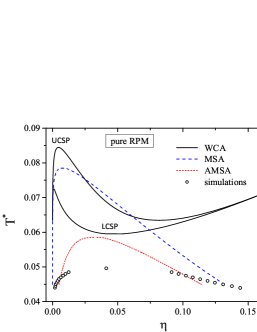
Figure 1: Phase diagram of a pure RPM fluid obtained theoretically in three approximations, i.e., the WCA approximation, the MSA, and the AMSA, and by simulations. Lines correspond to the theoretical results and symbols denote the results of MC simulations [23]. In the AMSA, the association constant $K^{0}=K^{0}_{OS}$ (see the text for details).

As expected, all these approximations lead to an essential overestimation of the critical temperature and an underestimation of the critical density in comparison with the computer simulations (see maxima on the curves). However, the vapour-liquid coexistence curve obtained in the AMSA approximation is noticeably better than in the WCA and MSA. The MSA yields slightly better results for the critical parameters than the WCA, especially for the critical density (see Table 1). At the same time, the diagram calculated in the WCA demonstrates a richer phase behavior of the RPM fluid. Apart from the vapour-liquid coexistence, the upper curve of the WCA phase diagram also contains the branch appearing at higher densities (for $\eta>0.08$), which may indicate another type of phase behaviour induced by the charge ordering. In addition, a lower region of the phase coexistence is found at low temperatures ($T^{*}<0.65$) with the corresponding lower critical point at $T_{L,c}^{*}=0.0595$ and $\eta_{L,c}=0.0472$ (see a minimum on the phase diagram). Therefore, the phase behaviour obtained in the WCA qualitatively differs from that described by the MSA and AMSA approaches. We note that the regions where a coexistence of more than two different phases are found by the WCA theory (at higher densities or at lower temperatures) appear due to a multiplicity of solutions for Eqs. (27) and (29). It means that at some temperatures we have found more than two coexisting densities, which correspond to the same pressure and chemical potential. However, it does not mean that all of the obtained phases can be considered as stable ones. In order to check our results for the phase stability we have analysed the spinodal curve calculated for the RPM fluid using the WCA approximation. In Fig. 2, one can observe that the above-mentioned regions are located lower than the spinodal curve, hence we show that they are unstable.

Also the lower critical point is analysed using the conditions to be held for a stable critical point

$$\left(\frac{\partial^{2}F}{\partial V^{2}}\right)_{T}=0,\qquad\left(\frac{\partial^{3}F}{\partial V^{3}}\right)_{T}=0,\qquad\left(\frac{\partial^{4}F}{\partial V^{4}}\right)_{T}>0.$$ (31)

We have found that at $T^{*}=T_{L,c}^{*}$ and $\eta=\eta_{L,c}$, the first two equations of (31) are satisfied, while the inequality is not satisfied. Thus, the lower critical point obtained in the WCA approximation is unstable as well.

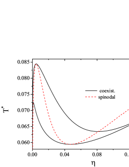
Figure 2: Phase diagram of a pure RPM fluid obtained in the WCA approximation. The coexistence curves are presented by solid lines and the spinodal is presented by a dashed line.

Table 1: The reduced vapour-liquid critical parameters, $T_{c}^{*}$ and $\rho_{c}^{*}$, for the restricted primitive model (RPM) obtained in the theory and by simulations.

Theory	$T_{c}^{*}$	$\rho_{c}^{*}$	Ref.
WCA appr.	$0.08446$	$0.0088$	[4, 3]
MSA	$0.07858$	$0.01449$	[3]
AMSA	0.0587	0.0590	[50]
simulation	0.0492	0.073	[23]

3.2 Phase diagrams of the RPM-HS mixture

The RPM-HS mixture undergoes the phase separation between a low-ionic-concentration phase and a high-ionic-concentration phase. Here, we address the phase diagrams of the RPM-HS mixture with $\sigma_{+}=\sigma_{-}=\sigma_{s}=\sigma$.

First, we focus on the WCA approximation. In this case, the expressions for the partial chemical potentials, $\nu_{i}$ and $\nu_{s}$, and for the pressure $P$ are given by Eqs. (9)-(11) taking into account Eq. (16). In Figs. 3 (a)-(b), we show the coexistence curves which are calculated at fixed pressures using Eqs. (27)-(29). The phase diagrams are presented in the $T^{*}$-$\eta$ and $T^{*}$-$c$ planes, where

$$T^{*}=k_{B}T\epsilon\sigma/q^{2},\qquad\eta=\eta_{i}+\eta_{s}=\pi\rho\sigma^{3}/6,\qquad c=\rho_{s}/\rho.$$ (32)

The selected pressures are higher than the critical pressure of the RPM in the WCA approximation ($P_{c}^{*}=P_{c}\varepsilon\sigma^{4}/q^{2}=7.85\times 10^{-5}$). It is seen in Fig. 3 (a) that the ($T^{*}$,$\eta$)-diagrams are of the shape similar to the phase diagram of the RPM obtained in the same approximation, i.e., they exhibit both the upper and the lower critical points. It is also observed that an increase of pressure shifts the coexistence region towards higher total number densities. The upper critical temperature is not affected essentially by the pressure, though a tendency to a small increase is noticed. On the other hand, an increase of the lower critical temperature is more significant. For ($T^{*}$,$c$)-diagrams in Fig. 3 (b), one can see the closed miscibility loops and the lower critical solution points (LCSP), the existence of which was also observed experimentally in [62] for ionic solutions in a non-polar solvent (the solution of $N_{4444}Br$ in toluene). However, it was shown in [62] that the phase transition related to the LCSP is located in a metastable region. Using the equations from Appendix A, we have calculated positions of the critical points and have checked for their stability. We have found that, like for the RPM fluid, the lower critical point of the RPM-HS mixture is unstable. The upper critical point is stable and moves toward higher concentrations of the solvent when the pressure increases. It should be noted that a solvent rich phase in Fig. 3 (b) corresponds to a lower-density branch of the coexistence curve in Fig. 3 (a) and vice versa.

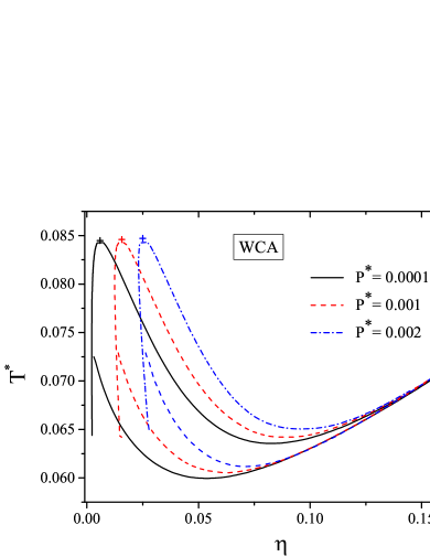
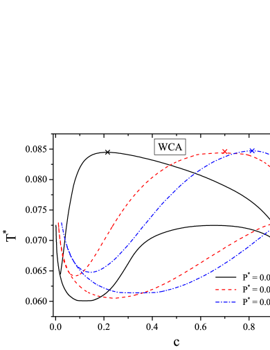
Figure 3: Coexistence curves of the RPM-HS mixture in $T^{*}$-$\eta$ (a) and $T^{*}$-$c$ (b) planes at constant reduced pressures in the WCA approximation. $T^{*}$, $\eta$, and $c$ are defined in Eq. (32), and $P^{*}=P\varepsilon\sigma^{4}/q^{2}$.

We have analysed the dependencies of the upper critical point parameters on the solvent concentration $c$ taking the RPM critical point as a reference (Figs. 4 (a)–(c)). One can see that an increase of the solvent concentration leads to a small increase of the critical temperature (Fig. 4 (a)) and to a significant increase of both the critical total packing fraction (Fig. 4 (b)) and the critical pressure (Fig. 4 (c)).

Figure 4: The RPM-HS mixture: critical temperature $T_{c}^{*}/T_{c}^{RPM}$ (a), critical packing fraction $\eta_{c}/\eta_{c}^{RPM}$ (b), and critical pressure $P_{c}^{*}/P_{c}^{RPM}$ (c) depending on the solvent concentration $c$ in the WCA approximation. $T_{c}^{RPM}$, $\eta_{c}^{RPM}$, and $P_{c}^{RPM}$ are the critical temperature, the critical packing fraction, and the critical pressure of a pure RPM fluid, respectively. $T^{*}$, $\eta$, and $c$ are defined in Eq. (32), and $P^{*}=P\varepsilon\sigma^{4}/q^{2}$.

Next, we have calculated the phase diagrams in the MSA. In this case, explicit expressions for the partial chemical potentials and pressure are obtained using Eqs. (9)-(11) together with (13)-(14). Figs. 5 (a)-(b) show the coexistence curves in the $T^{*}$-$\eta$ and $T^{*}$-$c$ planes obtained from Eqs. (27)-(29). The phase diagrams are presented at pressures above the MSA critical pressure for the RPM that is $P^{*}=9.64\times 10^{-5}$. The selected pressures are the same as in [31] (see Fig. 4 in [31]) where the MSA results for the RPM-HS mixture are presented. A visual comparison made between our and the above-mentioned results indicates their quantitative agreement in the region of temperatures $T_{c}^{*}>T^{*}>0.07$ for which the coexistence is found in [31]. In our case, at each value of pressure, the phase coexistence is found for a wider region of temperatures, i.e., for $T_{c}^{*}>T^{*}>0.05$ which, in turn, corresponds to wider regions of packing fractions and concentrations. Nevertheless, neither phase transition related to the LCSP nor closed miscibility loop is observed in the MSA. For all of the considered pressures, we have obtained only the upper critical points. For this type of phase transition, the obtained results qualitatively agree with the results of the WCA approximation. Quantitatively, the MSA produces a slightly lower critical temperature and a higher critical density than the corresponding critical parameters in the WCA approximation.

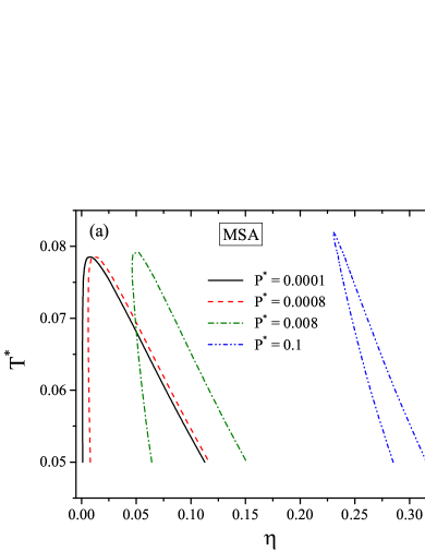
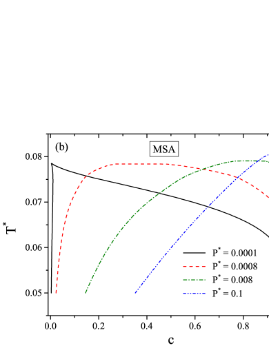
Figure 5: Coexistence curves of the RPM-HS mixture in $T^{*}$-$\eta$ (a) and $T^{*}$-$c$ (b) planes at constant reduced pressures in the MSA. $T^{*}$, $\eta$, and $c$ are defined in Eq. (32), and $P^{*}=P\varepsilon\sigma^{4}/q^{2}$.

Finally, we present the coexistence curves calculated using the AMSA theory. Then, the partial chemical potentials and pressure are given by Eqs. (21)-(26) supplemented by the solution of Eq. (19). The same as for the RPM, the association constant has been chosen to be $K^{0}=12K_{Eb}^{0}$. The phase diagrams in the $T^{*}$-$\eta$ and $T^{*}$-$c$ planes at constant pressures are shown in Figs 6 (a),(b). All the selected values of pressure are higher than the critical pressure of the RPM ($P_{c}^{*}=7.44\times 10^{-4}$). It is worth noting that the critical pressure of the pure ionic system obtained in the AMSA is by an order higher than the corresponding pressure found from the MSA and WCA theories. In general, the phase behaviour is qualitatively similar to that found in the MSA. The LCSP phase transitions have not been found in the AMSA either. Due to extreme flatness of the tops of coexisting curves obtained in the AMSA it is impossible to determine an exact location of the critical points. Although we can estimate the critical temperature with a rather good numerical accuracy, the critical densities and concentrations cannot be well defined. On the other hand, they can be estimated as half the sum of the densities (concentrations) in coexisting phases observed at the highest possible temperature below the critical temperature. The AMSA theory yields substantially lower values of the critical temperature and higher values of the critical total number density than the MSA. Moreover, the critical temperatures obtained from the AMSA theory fall within the region predicted by simulations [34]. It is worth noting that in [34], only the estimates of upper and lower bounds of the critical temperature are presented. Since the AMSA provides the prediction of critical points close to the critical points obtained from simulations, we compare our AMSA results with the coexisting curves obtained in simulations by Kristóf et al. [30] (see Figs.7 (a)-(b)) at the temperature $T^{*}=0.45$. As it is seen, the AMSA theory yields a reasonable agreement with the simulation results.

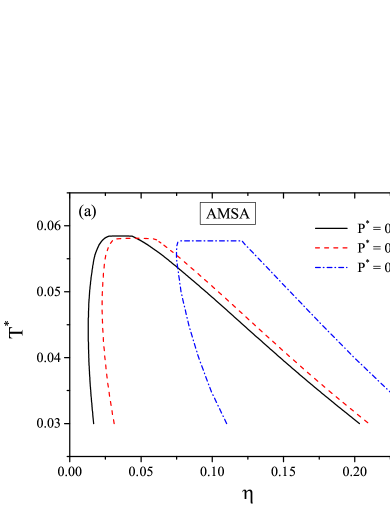
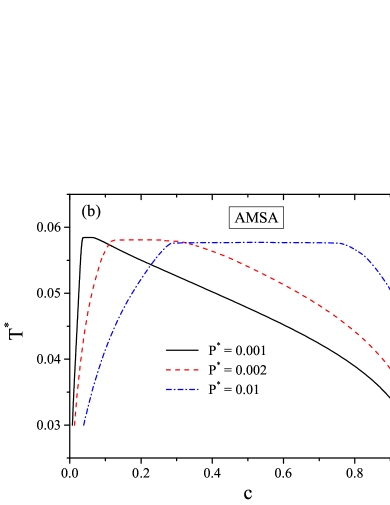
Figure 6: Coexistence curves of the RPM-HS mixture presented in $T^{*}$-$\eta$ (a) and $T^{*}$-$c$ (b) planes at constant reduced pressures in the AMSA. $T^{*}$, $\eta$, and $c$ are defined in Eq. (32), and $P^{*}=P\varepsilon\sigma^{4}/q^{2}$.

Figure 7: Coexistence curves of the RPM-HS mixture presented in $P^{*}$-$\rho^{*}$ (a) and $P^{*}$-$c$ (b) planes at constant temperature $T^{*}=0.045$. The lines are our AMSA results and the squares are the results of simulations [30]. $P^{*}=P\varepsilon\sigma^{4}/q^{2}$, $\rho^{*}=\rho\sigma^{3}$, and $T^{*}$, $c$ are defined in Eq. (32).

4 Conclusions

We have applied well-known theoretical approaches, i.e., the CV theory, the MSA, and the AMSA to the study of fluid-fluid phase equilibria in the model of ionic solutions that takes into account the presence of the solvent explicitly. Using the CV theory, we have found free energy, pressure and partial chemical potentials in the RPA for a rather general model that takes into consideration solvent-solvent and solvent-ion interactions beyond the hard core. In this paper, we have focused on RPM-HS mixture consisting of oppositely charged hard spheres and neutral hard spheres. Within the RPA, we arrive at free energy in the WCA approximation by exploiting the WCA regularization of the Coulomb potential inside the hard core [3] and at free energy in the ORPA/MSA by using the optimized regularization of the Coulomb potential [44]. It should be emphasised that the WCA approximation and the AMSA theory are applied to the study of the phase behaviour of the RPM-HS mixture for the first time. Despite the fact that the RPM-HS mixture had been previously studied by the MSA [31], in this paper we calculated the MSA phase diagrams for a wider region of thermodynamic parameters. Moreover, the calculation of the coexistence curves in the MSA serves as a verification of our results.

We have calculated the fluid-fluid coexistence curves using the equations of phase equilibrium. The three above-mentioned approximations produce qualitatively similar results for the phase diagrams, i.e., an increase of pressure shifts a fluid-fluid coexistence region towards higher total number densities and towards higher solvent concentrations and at the same time leads only to a small increase of the critical temperature. It should be noted that the equations of the phase equilibrium yield more complex phase diagrams in the WCA approximation compared to the MSA and AMSA. In particular, they consist of upper and lower branches that form a closed loop with the LCSP. However, the thermodynamic analysis shows that a lower branch and the corresponding critical point are unstable. Remarkably, the LCSP and a nearly closed miscibility loop located in the metastable region were reported for an ionic solution in a non-polar solvent (the solution of $N_{4444}Br$ in toluene) [62]. A quantitative comparison of the results obtained in the three approximations indicates that critical temperatures provided by the AMSA are lower than in the WCA and MSA, while critical total number densities are higher. As for a pure RPM, the AMSA approximation leads to the best agreement with simulation findings. However, this result is defined by the association constant, which in our study is chosen in the form proposed by Olaussen and Stell [58].

The next steps towards a theoretical description of the fluid-fluid phase behaviour in ionic solutions are to include other details of solvent-solvent and solvent-ion interactions, i.e., attraction/repulsion interactions beyond the hard core as well as a size (shape) asymmetry of ions and ion/solvent species. This work is now in progress using an analytical expression for the RPA free energy derived in Sec. 2. Another important issue is to go beyond the RPA in the study of explicit solvent models. This can be done within the framework of the CV theory. As it was shown in [18, 17, 19, 20], the CV approach is capable of reproducing, at least qualitatively, the effects of size and charge asymmetry on the vapour-liquid phase behaviour of the PMs, the solvent-free models of ionic solutions. In addition, the CV theory and the AMSA approach can be extended to the explicit solvent models which takes into account a non-spherical shape of solvent molecules.

Appendix A Equations for the critical points of a two-component mixture

The first two equations entering (30) expressed in terms of derivatives of the Helmholtz free energy are as follows [61]:

$$F_{2c}F_{2V}-F_{Vc}^{2}=0,$$

$$F_{3c}F_{2V}^{2}-3F_{V2c}F_{Vc}F_{2V}+3F_{2Vc}F_{Vc}^{2}-F_{3V}F_{2c}F_{Vc}=0,$$

where

$$F_{nVmc}=\frac{\partial^{n+m}F}{\partial V^{n}\partial c^{m}}$$

and $V$ and $c$ are the system volume and the solvent concentration, respectively.

The inequality in (30) is found to be

$$F_{4c}F_{2V}^{3}-4F_{2V}^{2}F_{Vc}F_{V3c}+6F_{2V}F_{Vc}^{2}F_{2V2c}-4F_{Vc}^{3}F_{3Vc}+F_{2c}F_{Vc}^{2}F_{4V}$$

$$-3F_{2V}^{2}F_{V2c}^{2}-12F_{Vc}^{2}F_{2Vc}^{2}-6F_{3V}F_{Vc}^{2}F_{V2c}+12F_{2V}F_{Vc}F_{2Vc}F_{V2c}$$

$$+12F_{2c}F_{Vc}F_{2Vc}F_{3V}-3F_{2c}^{2}F_{3V}^{2}>0.$$

For the RPM-HS mixture, we obtain in the WCA approximation

$$\beta F_{2V} = \frac{N}{V^{2}}\left(a_{0}-24\eta c^{2}i_{2}\right),$$

$$\beta F_{2c} = N\left(\tilde{a}_{1}-24\eta i_{2}\right),$$

$$\beta F_{Vc} = \frac{N}{V}24\eta ci_{2},$$

$$\beta F_{3V} = -\frac{N}{V^{3}}\left[a_{2}-72\eta c^{2}\left(i_{2}-16\eta ci_{3}\right)\right],$$

$$\beta F_{3c} = -N\left[a_{1}-2(24\eta)^{2}i_{3}\right],$$

$$\beta F_{2Vc} = -\frac{N}{V^{2}}48\eta c\left(i_{2}-24\eta ci_{3}\right),$$

$$\beta F_{V2c} = \frac{N}{V}24\eta\left(i_{2}-48\eta ci_{3}\right),$$

$$\beta F_{4V} = -\frac{N}{V^{4}}\left\{a_{3}+2a_{2}-144\eta c^{2}\left[2i_{2}-64\eta ci_{3}+(24\eta c)^{2}i_{4}\right]\right\},$$

$$\beta F_{4c} = -N\left[a_{11}-6(24\eta)^{3}i_{4}\right],$$

$$\beta F_{3Vc} = \frac{N}{V^{3}}144\eta c\left[i_{2}-48\eta ci_{3}+(24\eta c)^{2}i_{4}\right],$$

$$\beta F_{V3c} = -\frac{N}{V}4(24\eta)^{2}\left(i_{3}-36\eta ci_{4}\right),$$

$$\beta F_{2V2c} = -\frac{N}{V^{2}}48\eta\left[i_{2}-96\eta ci_{3}+3(24\eta c)^{2}i_{4}\right].$$

In the above equations, the following notations are used

$$a_{1} = \frac{1-2c}{c^{2}(1-c)^{2}},\quad\tilde{a}_{1}=\frac{1}{c(1-c)},\quad a_{11}=\frac{2(1-3c+3c^{2})}{c^{3}(1-c)^{3}},$$

$$a_{2} = \frac{2(1+7\eta+10\eta^{2}-10\eta^{3}+5\eta^{4}-\eta^{5})}{(1-\eta)^{5}},\quad a_{3}=\frac{24\eta(1+4\eta)}{(1-\eta)^{6}},$$

$$i_{n} = \frac{1}{\pi}\int_{0}^{\infty}\frac{y^{2}\sin(y)^{n}}{(T^{*}y^{3}+24\eta c\sin(y))^{n}}{\rm{d}}y,\qquad y=k\sigma_{i}.$$

References

References

- [1] G. Stell, J. Stat. Phys. 78 (1995) 197-238.
- [2] Y. Levin, M.E. Fisher, Physica A 225 (1996) 164-220.
- [3] J.-M. Caillol, Mol. Phys. 103 (2005) 1271-1283.
- [4] O.V. Patsahan, Condens. Matter Phys. 7 (2004) 35-52.
- [5] J.-M. Caillol, D. Levesque, J.-J. Weis, J. Chem. Phys. 116 (2002) 10794-10800.
- [6] A.-P. Hynninen, A.Z. Panagiotopoulos, Mol. Phys. 106 (2008) 2039-2051.
- [7] D. Saracsan, C. Rybarsch, W. Schröer. Z. Phys. Chem. 220 (2006) 1417-1437.
- [8] M. Wagner, O. Stanga, W. Schröer, Phys. Chem. Chem. Phys. 5 (2003) 3943-3950.
- [9] A. Butka, V.R. Vale, D. Saracsan, C. Rybarsch, W.C. Weiss, W. Schröer, Pure Appl.Phys. 80 (2008) 1613-1630.
- [10] W. Schröer and V.R. Vale, J. Phys.: Condens. Matter 21 (2009) 424119 (21pp).
- [11] W. Schröer, Contrib. Plasma Phys. 52 (2012) 78-88.
- [12] E. González-Tovar, Mol. Phys. 97 (1999) 1203-1206.
- [13] Y.V. Kalyuzhnyi, M.F. Holovko, V. Vlachy, J. Stat. Phys. 100 (2000) 243-265.
- [14] D.M. Zuckerman, M.E. Fisher, S. Bekiranov, Phys. Rev. E, 64 (2001) 011206-13.
- [15] M.N. Artyomov, V. Kobelev, A.B. Kolomeisky, J.Chem.Phys. 118 (2003) 6394-6402.
- [16] M.E. Fisher, J.-N. Aqua, S. Banerjee, Phys. Rev. Lett. 95 (2005) 135701-4.
- [17] O.V. Patsahan, I.M. Mryglod, T.M. Patsahan, J.Phys.: Condens. Matter 18 (2006) 10223-10235.
- [18] O. Patsahan, T.Patsahan, AIP Conf. Proc. 1198 (2009) 124-131.
- [19] O. V. Patsahan, T.M. Patsahan, Phys. Rev. E, 81 (2010) 031110-10.
- [20] O.V. Patsahan, I.M. Mryglod, Phase behaviour and criticality in primitive models of ionic fluids, in: Yu. Holovach (Ed.), Order, Disorder and Criticality. Advances Problems of phase transition theory, Singapore, Word Scientific, 2013, vol. 3, pp. 47-92.
- [21] P.J. Camp, G.N. Patey, J. Chem. Phys. 111 (1999) 9000-9008.
- [22] J.M. Romero-Enrique, G. Orkoulas, A.Z. Panagiotopoulos, M.E. Fisher, Phys. Rev. Lett. 85 (2000) 4558-4561.
- [23] Q. Yan, J.J. de Pablo, Phys. Rev. Lett. 86 (2001) 2054-7.
- [24] Q. Yan, J.J. de Pablo, Phys. Rev. Lett. 88 (2002) 095504-4.
- [25] Q. Yan, J.J. de Pablo, J. Chem. Phys. 116 (2002) 2967-2972.
- [26] A.Z. Panagiotopoulos, M.E. Fisher, Phys. Rev. Lett. 88 (2002) 045701-4.
- [27] A.Z. Panagiotopoulos, J.Chem.Phys. 116 (2002) 3007-3011.
- [28] D.W. Cheong, and A.Z. Panagiotopoulos, J. Chem. Phys. 119 (2003) 8526-8536.
- [29] Y.C. Kim, M.E. Fisher, and A.Z. Panagiotopoulos, Phys. Rev. Lett. 95 (2005) 195703-4.
- [30] T. Kristóf, D. Boda, I. Szalai, D. Henderson, J. Chem. Phys. 113 (2000) 7488-7491.
- [31] P.U. Kenkare, C.K. Hall, C. Caccamo, J. Chem. Phys. 103 (1995)8098-8110.
- [32] Y. Zhou, G. Stell, J. Chem. Phys. 102 (1995) 5796-5802.
- [33] Y. Zhou, S. Yeh, G. Stell, J. Chem. Phys. 102 (1995) 5785-5795.
- [34] J.C. Shelley, G.N. Patey, J. Chem. Phys. 110 (1999) 1633-1637.
- [35] O. Patsahan, I. Mryglod, Condens. Matter Phys. 9 (2006) 659-668.
- [36] O. Patsahan, I. Mryglod, J.-M. Caillol, J. Phys. Stud. 11 (2007) 133-141.
- [37] M.F. Holovko, Yu.V. Kalyuzhnyi, Mol. Phys. 73 (1991) 1145-1157.
- [38] L. Blum, O. Bernard, J. Stat. Phys., 79 (1995) 569-583.
- [39] O. Bernard, L. Blum, J. Chem. Phys., 104 (1996) 4746-4754.
- [40] H. C. Andersen, D. Chandler, J. Chem. Phys. 55 (1971) 1497-1504.
- [41] D. Chandler D., H.C. Andersen, J. Chem. Phys. 54 (1971) 26-33.
- [42] J. D. Weeks, D. Chandler, H.C. Andersen, J. Chem. Phys. 54 (1971) 5237-5247.
- [43] N.F. Carnahan, K. E. Starling, J. Chem. Phys. 51 (1969) 635-636
- [44] E. Waisman, J.L. Lebowitz, J. Chem. Phys. 52 (1970) 4307-4309.
- [45] A. Ciach, G. Stell, J. Mol. Liq. 87 (2000) 255-273.
- [46] M.F. Holovko, Concept of ion association in the theory of electrolyte solutions, in: D. Henderson, M. Holovko, A. Trokhymchuk (Eds.), Ionic Soft matter: Modern trends in theory and applications, Springer, Dordrecht, Netherlands, 2005, vol. 206, pp. 45-81.
- [47] M.S. Wertheim, J. Stat. Phys., 35 (1984) 19-34.
- [48] M.S. Wertheim, J. Stat. Phys., 35 (1984) 35-47.
- [49] M.F. Holovko, J. Mol. Liq., 96 (2002) 65-85.
- [50] J. Jiang, L. Blum, O. Bernard, J.M. Prausnitz, S.I. Sandler, J. Chem. Phys., 116 (2002) 7977-7982.
- [51] L. Blum, Mol. Phys., 30 (1975) 1529-1535.
- [52] E. Waisman, J.L. Lebowitz, J. Chem. Phys., 56 (1972) 3086-3093.
- [53] E. Waisman, J.L. Lebowitz, J. Chem. Phys., 56 (1972) 3093-3099.
- [54] L. Blum, J. Chem. Phys., 61 (1974) 2129-2133.
- [55] J.R. Solana, Perturbation Theories for the Thermodynamic Properties of Fluids and Solids, CRC Press, Taylor and Francis Group, 2013.
- [56] G. Stell, Y.Q. Zhou, J. Chem. Phys. 91 (1989) 3618-3623.
- [57] M. Holovko, T. Patsahan, O. Patsahan, J. Mol. Liq., 228 (2017) 215-223.
- [58] K. Olaussen, G. Stell, J. Stat. Phys. 62 (1991) 221-237.
- [59] F.O. Raineri, J.P. Routh, G. Stell, J. Phys. IV France, 10 (2000) Pr5-99–Pr5-104.
- [60] W. Ebeling, Z. Phys. Chem. (Leipzig), 238 (1968) 400-402.
- [61] J.S. Rowlinson, F.L.Swinton, Liquids and Liquid Mixtures, third ed., Butterworth Scientific, 1982.
- [62] H.R. Dittmar, W.H. Schröer, J. Phys.Chem. B, 113 (2009) 1249-1252.