Origin of diverse nematic orders in Fe-based superconductors:
45^∘ rotated nematicity in AFe₂As₂ (A=Cs, Rb)

Abstract

The origin of diverse nematicity and their order parameters in Fe-based superconductors have been attracting increasing attention. Recently, a new type of nematic order has been discovered in heavily hole-doped ($n_{d}=5.5$) compound AFe₂As₂ (A=Cs, Rb). The discovered nematicity has ${B_{2g}}$ (=$d_{xy}$) symmetry, rotated by $45^{\circ}$ from the ${B_{1g}}$ (=$d_{x^{2}-y^{2}}$) nematicity in usual compounds with $n_{d}\approx 6$. We predict that the “nematic bond order”, which is the symmetry-breaking of the correlated hopping, is responsible for the ${B_{2g}}$ nematic order in AFe₂As₂. The Dirac pockets in AFe₂As₂ is essential to stabilize the ${B_{2g}}$ bond order. Both ${B_{1g}}$ and ${B_{2g}}$ nematicity in A_1-xBa_xFe₂As₂ are naturally induced by the Aslamazov-Larkin many-body process, which describes the spin-fluctuation-driven charge instability. The present study gives a great hint to control the nature of charge nematicity by modifying the orbital character and the topology of the Fermi surface.

The electronic nematic state, which is the spontaneous rotational symmetry breaking in the many-body electronic states, appears in many Fe-based superconductors ARPES . Above the structural transition temperature $T_{\rm S}$, the electronic nematic susceptibility develops divergently, observed as the softening of shear modulus $C_{66}$ Yoshizawa ; Bohmer , and the enhancements of low-energy Raman spectrum Gallais ; Raman2 and in-plane anisotropy of resistivity $\Delta\rho$ Fisher . The mechanism of nematicity and its order parameter attract increasing attention, as a key to understand the pairing mechanism of high-$T_{\rm c}$ superconductivity. The intimate relationship between nematicity and magnetism has been discussed based on the spin-nematic scenarios Fernandes ; DHLee ; QSi ; Valenti ; Fang ; Fernandes-review ; C4 ; Khasanov and the orbital/charge-order scenarios Kruger ; PP ; WKu ; Onari-SCVC ; Onari-SCVCS ; Onari-form ; FeSe-Yamakawa ; Text-SCVC ; JP ; Fanfarillo ; Chubukov-RG .

Beyond the initial expectations, Fe-based superconductors exhibit very rich phase diagrams with nematicity and magnetism. In FeSe, for example, the nematic order does not accompany the magnetism at ambient pressure, whereas this nonmagnetic nematic phase is suppressed and replaced with the SDW phase by applying pressure FeSe-P1 ; FeSe-P2 . This phase diagram is understood in terms of the orbital-order scenario by assuming the pressure-induced $d_{xy}$-orbital hole-pocket FeSe-P3 . In the orbital/charge-order scenario, the orbital/charge order is driven by the spin fluctuations, due to the Aslamazov-Larkin (AL) vertex correction (VC) that describes the charge-spin mode coupling. The significance of the AL process has been clarified by several theoretical studies, especially by renormalization group studies Tsuchiizu-Ru1 ; Tsuchiizu-Cu ; Tsuchiizu-CDW ; Chubukov-RG ; Chubukov-RG2 ; Schmalian . However, the origin of the diverse electronic states associated with charge, orbital and spin degree of freedoms is not fully understood.

Until recently, all the discovered nematic orders in Fe-based superconductors have ${B_{1g}}$ (=$d_{x^{2}-y^{2}}$) symmetry, along the nearest Fe-Fe direction. Recently, however, nematic order/fluctuation with ${B_{2g}}$ (=$d_{xy}$) symmetry, rotated by $45^{\circ}$ from the conventional ${B_{1g}}$ nematicity, has been discovered in heavily hole-doped ($n_{d}=5.5$) compound AFe₂As₂ (A=Cs, Rb). Strong ${B_{2g}}$ nematic fluctuations and static order have been discovered by the NMR study CsFe2As2-nematic , the quasiparticle-interference by STM RbFe2As2-nematic , and the measurement of in-plane anisotropy of resistivity Shibauchi-B2g in RbFe₂As₂ ($T_{c}\sim 2.5$K) and CsFe₂As₂ ($T_{c}\sim 1.8$K). No SDW transition is observed in both compounds down to $T_{\rm c}$. CsFe2As2-HF ; Shibauchi-B2g . Surprisingly, both ${B_{1g}}$ and ${B_{2g}}$ nematic transitions are observed in Y-based Sato-BIg and Hg-based Murayama-BIIg cuprate superconductors, respectively, at the pseudogap temperature $T^{*}$. Theoretical studies of nematicity in cuprates have been performed by many authors Sachdev ; Fradkin ; Metzner ; Metzner2 ; Yamakawa-c ; PLee ; Pepin ; Kawaguchi-Cu ; Tsuchiizu-Cu . The discovery of unexpected ${B_{2g}}$ nematicity in both Fe-based and cuprate superconductors puts a severe constraint on the mechanism of nematicity.

In this paper, to reveal the origin of the ${B_{2g}}$ nematicity, we study the spin-fluctuation-driven charge nematicity in AFe₂As₂ by considering the higher-order VCs. We predict that the “nematic bond order”, given by the symmetry-breaking in the $d_{xy}$-orbital correlated hopping, is responsible for the ${B_{2g}}$ nematic order in AFe₂As₂. The Dirac pockets around X,Y points play essential role on the $B_{2g}$ bond order. With electron-doping, it is predicted that the ${B_{2g}}$ nematicity changes to the conventional ${B_{1g}}$ nematicity at the Lifshitz transition point, at which two Dirac pockets merge into one electron Fermi surface (FS). The diverse nematicity in A_1-xBa_xFe₂As₂ is naturally understood since the charge nematicity caused by the AL-VCs is sensitive to orbital character and topology of the FS. The present study gives a great hint to control the nature of nematicity in Fe-based superconductors.

First, we introduce the nematic order parameters. Figure 1 (a) shows B_1g nematic states due to orbital order ($n_{xz}\neq n_{yz}$). Here, the ($x,y$) axes are along the nearest Fe-Fe directions. The orbital order is the origin of the B_1g nematicity in Fe-based superconductors. Figure 1 (b) shows B_2g nematic state given by the next-nearest-neighbor (NNN) bond order, which corresponds to the modulation of the NNN correlated hopping $\delta t_{2}$. We propose that the B_2g bond order is the origin of the B_2g nematicity in AFe₂As₂, which has not been discussed in previous theoretical studies JP ; Metzner ; Metzner2 ; Sachdev .

We analyze the following two-dimensional eight-orbital $d$-$p$ Hubbard model with parameter $r$ Onari-form :

$$H_{\rm M}(r)=H^{0}+rH^{U},\ \ \$$ (1)

where $H^{0}$ is the unfolded tight-binding model derived from the first-principles calculation for CsFe₂As₂, which we introduce in the Supplemental Material (SM) A SM . $H^{U}$ is the first-principles screened Coulomb potential for $d$-electrons in BaFe₂As₂ Arita . Figure 1(c) shows the Fermi surfaces (FSs): The hole FS around M point (FS3) composed of $d_{xy}$-orbital is large, while the Dirac pockets near X and Y points (FS4,5) are small. The arrows denote the most important intra-$d_{xy}$-orbital nesting vectors. Below, we denote the five $d$-orbital $d_{3z^{2}-r^{2}}$, $d_{xz}$, $d_{yz}$, $d_{xy}$, $d_{x^{2}-y^{2}}$ as $l=1,2,3,4,5$.

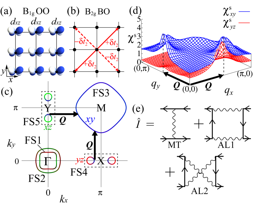
Figure 1: Schematic pictures of (a) ${B_{1g}}$ orbital order (OO), and (b) ${B_{2g}}$ bond order (BO). (c) FSs of the CsFe₂As₂ model in unfolded zone. The colors green, red and blue correspond to orbitals 2, 3 and 4, respectively. Each arrow denotes the significant intra-$d_{xy}$-orbital nesting vector $\bm{Q}=(0.53\pi,0)$. (d) ${{\bm{q}}}$ dependences of $\chi^{s}_{xy}({{\bm{q}}},0)$ and $\chi^{s}_{yz}({{\bm{q}}},0)$ given by the RPA. (e) Feynman diagrams of the irreducible four-point vertex $\hat{I}$. The wavy line is the fluctuation-mediated interaction $\hat{V}^{s,c}$

We calculate the spin (charge) susceptibilities ${\hat{\chi}}^{s(c)}(q)$ for $q=({{\bm{q}}},{\omega}_{m}=2m\pi T)$ based on the random-phase-approximation (RPA). The spin Stoner factor $\alpha_{s}$ is given by the maximum eigenvalue of $\hat{\Gamma}^{s}\hat{\chi}^{0}(\bm{q},0)$, where ${\hat{\Gamma}}^{s(c)}$ is the bare Coulomb interaction for the spin (charge) channel, and $\hat{\chi}^{0}$ is the irreducible susceptibilities given by the Green function without self-energy ${\hat{G}}(k)=[(i{\epsilon}_{n}-\mu){\hat{1}}-{\hat{h}}^{0}({{\bm{k}}})]^{-1}$ for $k=[{{\bm{k}}},{\epsilon}_{n}=(2n+1)\pi T]$. Here, ${\hat{h}}^{0}({{\bm{k}}})$ is the matrix expression of $H^{0}$ and $\mu$ is the chemical potential. Details of $\hat{\Gamma}^{s(c)}$, $\hat{\chi}^{s(c)}(q)$, and $\hat{\chi}^{0}(q)$ are explained in the SM A SM . We use $N=64\times 64$ ${{\bm{k}}}$-meshes and $512$ Matsubara frequencies, and fix the parameters $r=0.30$ and $T=0.03$ eV unless otherwise noted. Figure 1(d) shows the obtained spin susceptibility $\chi^{s}_{xy(yz)}({{\bm{q}}},0)\equiv\chi^{s}_{l,l;l,l}({{\bm{q}}},0)$ with $l=4$ ($l=3$) at $\alpha_{s}=0.93$. $\chi^{s}_{xy}$ is enlarged due to the intra-$d_{xy}$-orbital nesting, and it has the largest peak at ${{\bm{q}}}=\bm{Q}=(0.53\pi,0)$. In contrast, $\chi^{s}_{yz}$ is small since the intra-$d_{yz}$-orbital nesting is bad. Note that $\chi^{s}_{xy}\leq\chi^{s}_{yz}$ in LaFeAsO, BaFe₂As₂, and FeSe since two Dirac pockets (FS4 and FS5) merge into a usual electron pocket for $n_{d}\sim 6.0$.

Hereafter, we study the symmetry-breaking in the self-energy ($\Delta\hat{\Sigma}$) based on the density-wave (DW) equation introduced in Ref. Onari-form . We calculate both momentum- and orbital-dependences of $\Delta\Sigma_{l,l^{\prime}}^{{\bm{q}}}(k)$ self-consistently in order to analyze both orbital order and bond order on equal footing. To find the wavevector ${{\bm{q}}}$ of the DW state, we solve the following linearized DW equation:

$$\lambda_{{\bm{q}}}\Delta{\hat{\Sigma}}^{{\bm{q}}}(k)=\frac{T}{N}\sum_{k^{\prime}}{\hat{K}}^{\bm{q}}(k,k^{\prime})\Delta{\hat{\Sigma}}^{{\bm{q}}}(k^{\prime}),$$ (2)

where $\lambda_{{\bm{q}}}$ is the eigenvalue for the DW equation. The DW with wavevector ${{\bm{q}}}$ appears when $\lambda_{{\bm{q}}}=1$, and the eigenvector $\Delta\hat{\Sigma}^{{\bm{q}}}(k)$ gives the DW form factor. The kernel function $\hat{K}^{\bm{q}}(k,k^{\prime})$ Kawaguchi-Cu is given by

$${\hat{K}}^{\bm{q}}(k,k^{\prime})={\hat{I}}^{\bm{q}}(k,k^{\prime}){\hat{g}}^{\bm{q}}(k^{\prime}),$$ (3)

where $g^{\bm{q}}_{l,l^{\prime};m,m^{\prime}}(k)\equiv G_{l,m}\left(k+\frac{\bm{q}}{2}\right)G_{m^{\prime},l^{\prime}}\left(k-\frac{\bm{q}}{2}\right)$, and $\hat{I}^{\bm{q}}(k,k^{\prime})$ is the irreducible four-point vertex. It is given by the Ward identity $\hat{I}=\delta{\hat{\Sigma}}/\delta{\hat{G}}$, where $\hat{\Sigma}$ is one-loop self-energy conserving . The Feynman diagram of $\hat{I}^{\bm{q}}$ is shown in Fig. 1 (e): The first diagram corresponds to the Maki-Thompson (MT) term, and the second and the third diagrams are AL1 and AL2 terms, respectively. Its analytic expression is given in the SM ASM . Near the magnetic criticality, the charge-channel interaction due to the AL terms is strongly enhanced in proportion to $\sum_{p}\{\chi^{s}({{\bm{p}}},0)\}^{2}$, which is proportional to $\chi^{s}(\bm{Q},0)$ in two-dimensional systems. For this reason, the AL terms cause the spin-fluctuation-driven charge nematic order Onari-SCVC ; Onari-form ; Tsuchiizu-Cu ; Tsuchiizu-Ru1 ; Tsuchiizu-CDW .

The Hartree-Fock (HF) term, which is the first order term with respect to ${\hat{\Gamma}}^{s,c}$, is included in the MT term. As well-known, the HF term suppresses conventional charge DW order ($\Delta\Sigma=$const), whereas both ${B_{1g}}$ and ${B_{2g}}$ bond orders are not suppressed. Here, we drop the ${\epsilon}_{n}$-dependence of $\Delta{\hat{\Sigma}}^{{\bm{q}}}(k)$ by the analytic continuation (${\epsilon}_{n}\rightarrow{\epsilon}$) and putting ${\epsilon}=0$ Onari-form . This approximation leads to slight overestimation of $\lambda_{{\bm{q}}}$.

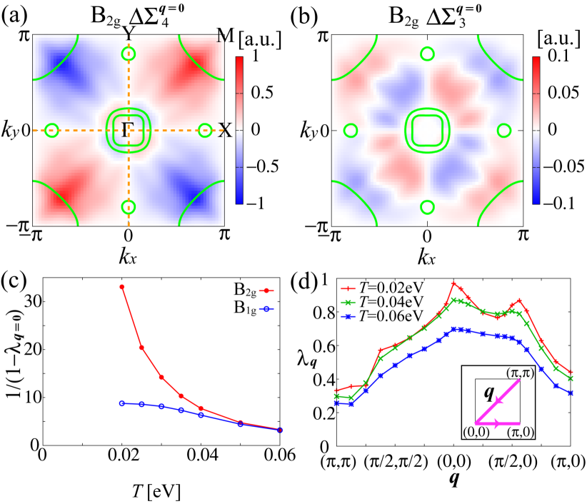
Figure 2: (a,b) ${B_{2g}}$ symmetry form factors at ${{\bm{q}}}={\bm{0}}$ obtained as the largest eigenvalue. The primary form factor on $d_{xy}$ orbital, $\Delta\Sigma_{4}^{\bm{0}}\propto\sin k_{x}\sin k_{y}$, gives the bond order. Orange dotted lines represent the symmetry nodes. (c) The strengths of nematic fluctuations $1/(1-\lambda_{\bm{q}=\bm{0}})$ for ${B_{2g}}$ and ${B_{1g}}$ symmetries as a function of $T$. (d) $\bm{q}$ dependences of the maximum eigenvalue at $T=0.02$eV, $0.04$eV, and $0.06$eV.

Figures 2(a) and 2(b) show the obtained form factors at ${{\bm{q}}}={\bm{0}}$, $\Delta\Sigma^{\bm{0}}_{4}({{\bm{k}}})\equiv\Delta\Sigma^{\bm{0}}_{4,4}({{\bm{k}}})$ and $\Delta\Sigma^{\bm{0}}_{3}({{\bm{k}}})\equiv\Delta\Sigma^{\bm{0}}_{3,3}({{\bm{k}}})$, for the largest eigenvalue $\lambda=0.93$. (The absolute value of $\Delta\hat{\Sigma}^{{{\bm{q}}}}$ is meaningless.) The obtained form factor has ${B_{2g}}$-symmetry since the symmetry relation $\Delta\Sigma^{\bm{0}}_{4}(k_{x},k_{y})\propto\sin k_{x}\sin k_{y}$ holds. The relation $|\Delta\Sigma_{xy}|\gg|\Delta\Sigma_{yz(xz)}|$ means that the primary nematic order is the “next-nearest-neighbor bond order for $d_{xy}$ orbital”, which is shown in Fig. 1 (b). The obtained ${B_{2g}}$ bond order is consistent with the experimental ${B_{2g}}$ nematicity in AFe₂As₂ CsFe2As2-nematic ; Shibauchi-B2g ; RbFe2As2-nematic . The second largest eigenvalue $\lambda=0.88$ corresponds to the ${B_{1g}}$ nematic bond order, details of which we explain in the SM B SM .

As explained in the SM C SM , the nematic susceptibility with respect to the form factor $\Delta\hat{\Sigma}^{\bm{q}}$ is given as ${\hat{\chi}}^{\Delta\Sigma}({{\bm{q}}})\propto(1-\lambda_{\bm{q}})^{-1}$ that diverges at $\lambda_{\bm{q}}=1$. Figure 2(c) shows the $T$ dependences of $(1-\lambda_{\bm{0}})^{-1}$ for both ${B_{2g}}$ and ${B_{1g}}$ symmetry solutions. We see that $(1-\lambda_{\bm{0}})^{-1}$ for the ${B_{2g}}$ symmetry shows the Curie-Weiss behavior and dominates over that for the ${B_{1g}}$ symmetry. These results are consistent with the experimental nematic susceptibility CsFe2As2-nematic ; Shibauchi-B2g . In Fig. 2(d), we show the ${{\bm{q}}}$ dependences of the largest eigenvalue at $T=0.02$eV, $0.04$eV, and $0.06$eV. It is confirmed that the nematic susceptibility actually has the maximum peak at ${{\bm{q}}}=\bm{0}$, and the symmetry of form factor is ${B_{2g}}$.

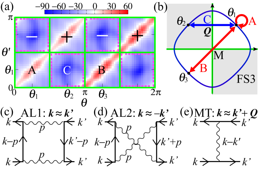
Figure 3: (a) $K_{\rm FS3}(\theta,\theta^{\prime})$ on FS3 given by all vertex terms. The green lines denote the ${B_{2g}}$ symmetry nodes. A, B, and C represent the pairs of Fermi points $(\theta_{1},\theta_{1})$, ($\theta_{3},\theta_{1}$), and $(\theta_{2},\theta_{1})$, respectively: $\theta_{1}\equiv\pi/4$, $\theta_{2}\equiv 3\pi/4$, and $\theta_{3}\equiv 5\pi/4$. (b) $B_{2g}$ symmetry order ($\Delta\Sigma({{\bm{k}}})\propto\sin k_{x}\sin k_{y}$) driven by attractive (repulsive) interaction for pairs A and B (pair C). (c,d,e) $\hat{I}^{\bm{0}}(k,k^{\prime})$ given by AL1 term, AL2 term, and MT term. Two AL terms give strong attractive interaction for $({{\bm{k}}},\pm{{\bm{k}}})$, shown as red line regions in panel (a). The MT gives repulsive interaction for pair C, due to spin fluctuations at ${\bm{Q}}\approx(0.5\pi,0)$.

In order to understand the origin of the ${B_{2g}}$ nematic bond order, we analyze the momentum-dependence of the kernel function for $d_{xy}$ orbital. Figure 3 (a) shows $K_{\rm FS3}(\theta,\theta^{\prime})\equiv T\sum_{n^{\prime}}K^{\bm{0}}_{4,4;4,4}({{\bm{k}}}(\theta),{\epsilon}_{n},{{\bm{k}}}(\theta^{\prime}),{\epsilon}_{n^{\prime}})|_{{{\epsilon}_{n}}\rightarrow 0}$ given by the summation of the AL1, AL2, and MT terms on the FS3. Here, $\theta$ and $\theta^{\prime}$ denote the azimuthal angles (from the M point) of ${{\bm{k}}}$ and ${{\bm{k}}}^{\prime}$ on the FS3, respectively. Now, we define the pairs of Fermi points A$=(\theta_{1},\theta_{1})$, B$=(\theta_{3},\theta_{1})$, and C$=(\theta_{2},\theta_{1})$, where $\theta_{1}\equiv\pi/4$, $\theta_{2}\equiv 3\pi/4$, and $\theta_{3}\equiv 5\pi/4$. For these pairs $K_{\rm FS3}(\theta,\theta^{\prime})$ becomes large in magnitude. The green lines denote the nodes of ${B_{2g}}$ symmetry $(\theta,\theta^{\prime}=\frac{\pi}{2}n)$. The positive $K_{\rm FS3}(\theta,\theta^{\prime})$ for the pairs A and B give attractive interactions between the same $({{\bm{k}}}_{1},{{\bm{k}}}_{1})$ and the opposite $(-{{\bm{k}}}_{1},{{\bm{k}}}_{1})$ momenta in Eq. (2), respectively, where ${{\bm{k}}}_{i}\equiv{{\bm{k}}}(\theta_{i})$ $(i=1,2,3)$. On the other hand, the negative $K_{\rm FS3}(\theta,\theta^{\prime})$ for the pair C gives the repulsive interaction between $({{\bm{k}}}_{2},{{\bm{k}}}_{1})$. As we show in Fig. 3 (b), this checkerboard-type sign structure of $K_{\rm FS3}(\theta,\theta^{\prime})$, which is positive (negative) for pairs A and B (pair C), favors the ${B_{2g}}$ symmetry bond order $\Delta\Sigma^{\bm{0}}_{4}({{\bm{k}}})\propto\sin k_{x}\sin k_{y}$.

We briefly explain the microscopic origin of the checkerboard-type sign structure in $K_{\rm FS3}(\theta,\theta^{\prime})$. The positive $K_{\rm FS3}(\theta,\theta^{\prime})$ along $\theta^{\prime}=\theta$ in Fig. 3 (a) (including the pair A) originates from the AL1 term, since the particle-hole channel $\phi_{\mbox{p-h}}\equiv T\sum_{p}G_{4,4}(k-p)G_{4,4}(k^{\prime}-p)$ shown in Fig. 3 (c) takes large positive value for ${{\bm{k}}}^{\prime}={{\bm{k}}}$, as we explain in the SM D SM . Also, the positive $K_{\rm FS3}(\theta,\theta^{\prime})$ along $\theta^{\prime}=\theta+\pi$ (including the pair B) originates from the AL2 term, since the particle-particle (Cooper) channel $\phi_{\rm p\mbox{-}p}\equiv T\sum_{p}G_{4,4}(k-p)G_{4,4}(k^{\prime}+p)$ shown in Fig. 3 (d) takes large positive value for ${{\bm{k}}}^{\prime}=-{{\bm{k}}}$. On the other hand, the negative $K_{\rm FS3}(\theta_{2},\theta_{1})$ at the pair C stems from the MT term in Fig. 3 (e). This is because $\hat{V}^{s}(k-k^{\prime})\propto\hat{\chi}^{s}(k-k^{\prime})$ in the MT term becomes maximum for $({{\bm{k}}},{{\bm{k}}}^{\prime})=({{\bm{k}}}_{2},{{\bm{k}}}_{1})$ since ${{\bm{k}}}_{2}-{{\bm{k}}}_{1}$ coincides with the nesting vector ${{\bm{Q}}}$.

To summarize, both ${B_{1g}}$ and ${B_{2g}}$ nematicities can be induced by the AL terms, since they give attractive interaction for both $\theta\approx\theta^{\prime}$ and $\theta\approx\theta^{\prime}+\pi$. In fact, both the nematic susceptibilities $(1-\lambda_{{{\bm{q}}}})^{-1}$ for the ${B_{1g}}$ and the ${B_{2g}}$ increase as shown in Fig. 2 (c), consistently with recent experimentShibauchi-B2g . In the present model with spin fluctuations at ${\bm{Q}}\approx(0.5\pi,0)$, the ${B_{2g}}$ nematic order is assisted by the MT term. The magnitude of the AL kernel function dominates over that of the MT kernel function as we explain in SM D SM . For this reason, the eigenvalue of the DW equation $\lambda_{{\bm{q}}}$ can be larger than that of the Eliashberg gap equation, in which the kernel contains only the MT term Norman . We predict that the ${B_{2g}}$ nematicity is closely tied to the Dirac pockets, which give the main spin fluctuations in AFe₂As₂.

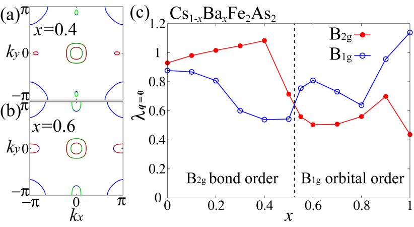
Figure 4: (a) FSs for $x=0.4$ and (b) FSs for $x=0.6$ in the Cs_1-xBa_xFe₂As₂ model. (c) $x$ dependences of $\lambda$ for ${B_{2g}}$- and ${B_{1g}}$ symmetry obtained in the Cs_1-xBa_xFe₂As₂ model.

Here, we discuss the doping-dependence of the nematicity: We introduce reliable model Hamiltonian for Cs_1-xBa_xFe₂As₂, by interpolating between CsFe₂As₂ model and BaFe₂As₂ model with the ratio $1-x:x$. With increasing $x$, the FSs with four Dirac pockets in Fig. 4(a) for $x=0.4$ change to the FSs with two electron pockets in Fig. 4(b) for $x=0.6$. In this model, the Lifshitz transition occurs at $x_{c}\approx 0.5$.

Figure 4(c) shows $x$ dependences of $\lambda_{\bm{q}=\bm{0}}$ for the ${B_{2g}}$ and the ${B_{1g}}$ symmetries in the Cs_1-xBa_xFe₂As₂ model, in which value of $r$ is fixed to 0.30. For $x<x_{c}$, the ${B_{2g}}$ bond order $\pm\delta t_{2}$ shown in Fig. 1 (b) is dominant over the ${B_{1g}}$ orbital order, since the former is driven by strong spin fluctuations in $d_{xy}$ orbital. For $x>x_{c}$, the ${B_{1g}}$ orbital order $n_{xz}\neq n_{yz}$ in Fig. 1(a) becomes dominant, because of the strong spin fluctuations in $d_{xz,yz}$ orbitals due to the nesting between electron- and hole-FSs Onari-SCVC ; Onari-SCVCS ; FeSe-Yamakawa , as we briefly explain in the SM E SM . Thus, the present theory naturally explains both the ${B_{1g}}$ nematicity in non-doped $(n_{d}\approx 6)$ systems and ${B_{2g}}$ nematicity in heavily hole-doped compounds in a unified way, by focusing on the impact of the Lifshitz transition.

The sudden decrease of $\lambda_{{\bm{0}}}^{\rm B_{2g}}$ at the Lifshitz transition point in Fig. 4 (c) indicates that the Dirac pockets are essential for the $B_{2g}$ nematicity, in spite of their small size. To verify this, we calculate $\chi^{s}_{xy}(q)$ by dropping the contribution from the rectangular areas around X,Y points shown in Fig. 1 (c): Then, as shown in Fig. 5 (a), the peak at ${{\bm{Q}}}=(0.53\pi,0)$ of $\chi^{s}_{xy}(q)$ in Fig. 1 (d) shifts to ${{\bm{Q}}}^{\prime}=(0.56\pi,0.56\pi)$, which is the intra-FS3 nesting vector. In this case, $K_{\rm FS3}(\theta,\theta^{\prime})$ due to MT term takes large negative value for $\theta\approx\theta_{a}$ and $\theta^{\prime}\approx\theta_{a}^{\prime}$ in Fig. 5 (b), and therefore $B_{1g}$ bond order emerges: $\lambda_{\bm{0}}^{B_{1g}}=0.82$ and $\lambda_{\bm{0}}^{B_{2g}}=0.77$. To summarize, the ${B_{2g}}$ nematicity in AFe₂As₂ is closely tied to the emergence of the Dirac pockets at the Lifshitz transition. Thus, we can control the nematicity by changing the topology and orbital character of the FSs.

Recently, the ${B_{2g}}$ vestigial nematic order has been proposed in Ref. Fernandes-B2g ; Si-B2g based on the real-space picture, whereas the double stripe magnetism (${{\bm{q}}}=(\pi/2,\pi/2)$) has not been observed yet. Thus, it is an important future issue to determine the mechanism of ${B_{2g}}$ nematicity.

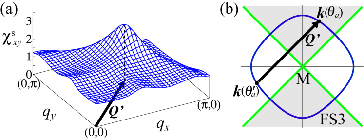
Figure 5: (a) $\chi^{s}_{xy}(q)$ for $r=0.36$ (${\alpha}_{S}=0.90$) given by dropping the contribution from the Dirac pockets. (b) $B_{1g}$ nematic order with green symmetry nodes and gray negative region on FS3 due to the intra-FS nesting $\bm{Q}^{\prime}\approx(0.6\pi,0.6\pi)$.

In summary, we studied the rich variety of nematic orders realized in $A_{1-x}$Ba_xFe₂As₂ (A=Cs, Rb) by solving the DW equation with AL- and MT-VCs . At $x=0$, the ${B_{2g}}$ bond order is driven by the spin fluctuations in $d_{xy}$ orbital. With increasing $x$, the ${B_{2g}}$ nematicity suddenly changes to ${B_{1g}}$ orbital nematicity ($n_{xz}-n_{yz}$) at the Lifshitz transition point, consistently with recent experiment Shibauchi-B2g . Both the FS orbital character and the FS topology are key ingredients not only to understand the diverse nematicity, but also to control the nature of nematicity in Fe-based superconductors. The present theory will give useful hints to understand recently-discovered rich nematic orders in cuprate superconductors Sato-BIg ; Murayama-BIIg .

We stress that the present DW equations satisfy the criteria of the “conserving approximation (CA)” by introducing the self-energy in $G$’s Baym1 ; Baym2 ; ROP . The great merit of the CA is that the macroscopic conservation laws are satisfied rigorously. This merit is important to avoid unphysical results. In the SM F SM , we improve the present theory within the framework of the CA, by introducing the self-energy given by the fluctuation-exchange (FLEX) approximation. The obtained ${{\bm{q}}}$-dependences of $\lambda_{{\bm{q}}}$ and ${B_{2g}}$ symmetry form factor are essentially similar to Fig. 2. Thus, the main results of the present study are justified within the framework of the CA.

[Supplementary Material]
Origin of diverse nematic orders in Fe-based superconductors:
45^∘ rotated nematicity in AFe₂As₂ (A=Cs, Rb)

Seiichiro Onari and Hiroshi Kontani

Department of Physics, Nagoya University, Nagoya 464-8602, Japan

I.1 A: Eight-orbital models for AFe₂As₂ and BaFe₂As₂

Here, we introduce the eight-orbital $d$-$p$ models for CsFe₂As₂ and BaFe₂As₂ analyzed in the main text. We first derived the first principles tight-binding models using the WIEN2k and WANNIER90 codes. Next, we introduce the $k$-dependent energy shifts for orbital $l$, $\delta E_{l}$, by introducing the intra-orbital hopping parameters, as we explain in Refs. S-FeSe-Yamakawa ; S-FeSe-Onari . For the CsFe₂As₂ model, we shift the $d_{xy}$-orbital band [$d_{xz/yz}$-orbital band] at ($\Gamma$, M, Y/X) points by ($0$, $+0.4$, $0$) [($-0.4$, $0$, $+0.1$)] in unit eV. For the BaFe₂As₂ model, we do not introduce any energy shifts. Figure S1 shows the bandstructures of the obtained (a) CsFe₂As₂ model and (b) BaFe₂As₂ model.

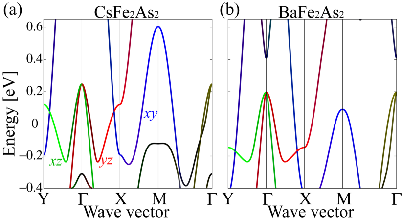
Figure S1: Bandstructures of the eight-orbital models for (a) CsFe₂As₂ and (b) BaFe₂As₂.

Next, we explain the multiorbital Coulomb interaction. The bare Coulomb interaction for the spin channel in the main text is

$$(\Gamma^{\mathrm{s}})_{l_{1}l_{2},l_{3}l_{4}}=\begin{cases}U_{l_{1},l_{1}},&l_{1}=l_{2}=l_{3}=l_{4}\\ U_{l_{1},l_{2}}^{\prime},&l_{1}=l_{3}\neq l_{2}=l_{4}\\ J_{l_{1},l_{3}},&l_{1}=l_{2}\neq l_{3}=l_{4}\\ J_{l_{1},l_{2}},&l_{1}=l_{4}\neq l_{2}=l_{3}\\ 0,&\mathrm{otherwise}.\end{cases}$$ (S1)

Also, the bare Coulomb interaction for the charge channel is

$$({\hat{\Gamma}}^{\mathrm{c}})_{l_{1}l_{2},l_{3}l_{4}}=\begin{cases}-U_{l_{1},l_{1}},&l_{1}=l_{2}=l_{3}=l_{4}\\ U_{l_{1},l_{2}}^{\prime}-2J_{1_{1},l_{2}},&l_{1}=l_{3}\neq l_{2}=l_{4}\\ -2U_{l_{1},l_{3}}^{\prime}+J_{l_{1},l_{3}},&l_{1}=l_{2}\neq l_{3}=l_{4}\\ -J_{1_{1},l_{2}},&l_{1}=l_{4}\neq l_{2}=l_{3}\\ 0.&\mathrm{otherwise}.\end{cases}$$ (S2)

Here, $U_{l,l}$, $U_{l,l^{\prime}}^{\prime}$ and $J_{l,l^{\prime}}$ are the first principles Coulomb interaction terms for $d$-orbitals of BaFe₂As₂ given in Ref. S-Arita .

Using the multiorbital Coulomb interaction, the spin (charge) susceptibility in the RPA is given by

$${\hat{\chi}}^{s(c)}(q)={\hat{\chi}}(q)[1-{\hat{\Gamma}}^{s(c)}{\hat{\chi}^{0}(q)}]^{-1},$$ (S3)

where irreducible susceptibilities is

$$\chi^{0}_{l,l^{\prime};m,m^{\prime}}(q)=-\frac{T}{N}\sum_{k}G_{l,m}(k+q)G_{m^{\prime},l^{\prime}}(k).$$ (S4)

Here, ${\hat{G}}(k)$ is the multiorbital Green function introduced in the main text. The $b$-channel interaction ($b=s,c$) given by the RPA is $\hat{V}^{b}(q)=\hat{\Gamma}^{b}+\hat{\Gamma}^{b}\hat{\chi}^{b}(q)\hat{\Gamma}^{b}$.

As shown by the Feynman diagram in Fig. 1 (e), $\hat{I}^{\bm{q}}(k,k^{\prime})$ is given as

$$\!\!\!\!\!\!\!\!\!\!\!I^{\bm{q}}_{l,l^{\prime};m,m^{\prime}}(k,k^{\prime})=\sum_{b=s,c}\left[\frac{a^{b}}{2}V^{b}_{l,m;l^{\prime},m^{\prime}}(k-k^{\prime})\right.$$

$$-\frac{T}{N}\!\!\!\!\sum_{p,l_{1},l_{2},m_{1},m_{2}}\!\!\!\!\!\!\!\!\!\!\frac{a^{b}}{2}V^{b}_{l,l_{1};m,m_{2}}\left(p+\frac{{{\bm{q}}}}{2}\right)V^{b}_{m^{\prime},l_{2};l^{\prime},m_{1}}\left(p-\frac{{{\bm{q}}}}{2}\right)$$

$$\qquad\qquad\times G_{l_{1},m_{1}}(k-p)G_{l_{2},m_{2}}(k^{\prime}-p)$$

$$-\frac{T}{N}\!\!\!\!\sum_{p,l_{1},l_{2},m_{1},m_{2}}\!\!\!\!\!\!\!\!\!\!\frac{a^{b}}{2}V^{b}_{l,l_{1};l_{2},m^{\prime}}\left(p+\frac{{{\bm{q}}}}{2}\right)V^{b}_{m_{2},m;l^{\prime},m_{1}}\left(p-\frac{{{\bm{q}}}}{2}\right)$$

$$\qquad\qquad\left.\times G_{l_{1},m_{1}}(k-p)G_{l_{2},m_{2}}(k^{\prime}+p)\right],$$

(S5)

where $a^{s(c)}=3\ (1)$ and $p=({{\bm{p}}},{\omega}_{l})$. In Eq. (S5), the first line corresponds to the Maki-Thompson (MT) term, and the second and the third lines give AL1 and AL2 terms, respectively. Double-counting second-order terms with respect to $\hat{\Gamma}^{s(c)}$ have to be subtracted.

I.2 B: ${B_{1g}}$ bond ordered state

Figures S2(a) and S2(b) show the form factors for the second largest eigenvalue $\lambda=0.88$. The obtained solution has ${B_{1g}}$-symmetry since the symmetry relation $\Delta\Sigma^{\bm{0}}_{4}(k_{x},k_{y})\propto\cos k_{x}-\cos k_{y}$ holds. This corresponds to the nearest-neighbor bond order for $d_{xy}$ orbital. This ${B_{1g}}$ bond order induces small secondary orbital order with ${B_{1g}}$ symmetry as shown in Fig. 1 (a).

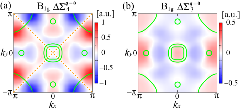
Figure S2: (a,b) ${B_{1g}}$ symmetry form factors at ${{\bm{q}}}={\bm{0}}$ obtained as the second largest eigenvalue. The primary form factor on $d_{xy}$ orbital, $\Delta\Sigma_{4}^{\bm{0}}\propto\cos k_{x}-\cos k_{y}$, gives the nearest-neighbor bond order. Orange dotted lines represent the symmetry nodes.

I.3 C: Nematic susceptibility

Next, we discuss the DW susceptibility with respect to the form factor $\Delta\hat{\Sigma}$; ${\hat{\chi}}^{\Delta\Sigma}$. By including both AL and MT vertex terms, it is given as

$$\chi^{\Delta\Sigma}_{l,l^{\prime};m,m^{\prime}}(q) = -\frac{T^{2}}{N^{2}}\sum_{k,k^{\prime}}\Delta\Sigma^{-\bm{q}}_{l,l^{\prime}}(-{{\bm{k}}})P^{\bm{q}}_{l,l^{\prime};m,m^{\prime}}(k,k^{\prime})$$ (S6)

$$\times\Delta\Sigma^{\bm{q}}_{m,m^{\prime}}({{\bm{k}}}^{\prime}),$$

where $\hat{P}^{\bm{q}}(k,k^{\prime})=\hat{g}^{\bm{q}}(k)[\delta_{k,k^{\prime}}+\hat{K}^{\bm{q}}(k,k^{\prime})+\frac{T}{N}\sum_{k^{\prime\prime}}\hat{K}^{\bm{q}}(k,k^{\prime\prime})\hat{K}^{\bm{q}}(k^{\prime\prime},k^{\prime})+\cdots]$. In Fig. S3, we shown the Feynman diagram for $\hat{P}^{\bm{q}}(k,k^{\prime})$, in which higher-order MT and AL terms are included. Using the Eq. (2), we can show that

$$\hat{\chi}^{\Delta\Sigma}(q)=(1-\lambda_{\bm{q}})^{-1}\frac{-T}{N}\sum_{k}\Delta\hat{\Sigma}^{-\bm{q}}(-{{\bm{k}}})\hat{g}^{\bm{q}}(k)\Delta\hat{\Sigma}^{\bm{q}}({{\bm{k}}}).$$

Thus, the DW with wavevector ${{\bm{q}}}$ emerges when ${\hat{\chi}}^{\Delta\Sigma}({{\bm{q}}})\propto(1-\lambda_{\bm{q}})^{-1}$ diverges.

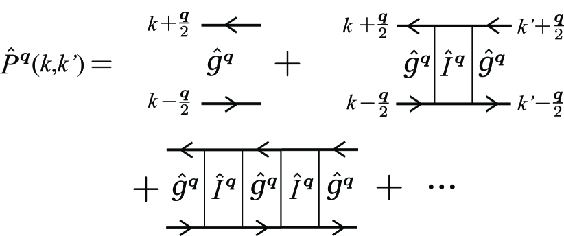
Figure S3: Feynman diagrams of the two-particle Green function $\hat{P}^{\bm{q}}(k,k^{\prime})$. The irreducible four-point vertex $\hat{I}^{\bm{q}}(k,k^{\prime})$ is introduced in Fig. 1 (g) in the main text.

I.4 D: Detailed explanation for the kernel function

In Fig. 3 (a) in the main text, we show the momentum-dependence of the kernel function $K_{\rm FS3}(\theta,\theta^{\prime})$ given by the all vertex terms. Here, we discuss the contribution from each vertex term. Figure S4 (a) shows $K_{\rm FS3}(\theta,\theta^{\prime})$ given by the AL1 term. The positive $K_{\rm FS3}(\theta,\theta^{\prime})$ in the line region $\theta^{\prime}\sim\theta$ $({i.e.},\ {{\bm{k}}}={{\bm{k}}}^{\prime})$ including the pair A comes from the particle-hole channel $\phi_{\mbox{p-h}}\equiv T\sum_{p}^{|{\omega}_{l}|<{\omega}_{c}}G_{4,4}(k-p)G_{4,4}(k^{\prime}-p)$. Here, the cutoff energy ${\omega}_{c}\ll E_{\rm F}$ corresponds to energy-scale of ${\hat{\chi}}^{s}$ in $\hat{V}^{s}$. It is easy to show that $\phi_{\mbox{p-h}}$ takes large positive value for ${{\bm{k}}}={{\bm{k}}}^{\prime}$ in the case of ${\omega}_{c}\ll E_{\rm F}$.

Figure S4 (b) shows $K_{\rm FS3}(\theta,\theta^{\prime})$ given by the AL2 term. The positive $K_{\rm FS3}(\theta,\theta^{\prime})$ in the line region $\theta^{\prime}=\theta+\pi$ $({i.e.},\ {{\bm{k}}}=-{{\bm{k}}}^{\prime})$ including the pair B stems from the particle-particle (Cooper) channel $\phi_{\rm p\mbox{-}p}\equiv T\sum_{p}^{|{\omega}_{l}|<{\omega}_{c}}G_{4,4}(k-p)G_{4,4}(k^{\prime}+p)\propto\sum_{\bm{p}}\frac{1-f(\xi_{4}({{\bm{k}}}-\bm{p}))-f(\xi_{4}({{\bm{k}}}^{\prime}+\bm{p}))}{\xi_{4}({{\bm{k}}}-\bm{p})+\xi_{4}({{\bm{k}}}^{\prime}+\bm{p})}$, which diverges logarithmically for ${{\bm{k}}}=-{{\bm{k}}}^{\prime}$ at $T=0$. Here, $f({\epsilon})$ is Fermi distribution function, $\xi_{4}({{\bm{k}}})$ is $d_{xy}$-orbital hole-band dispersion.

Figure S4(c) shows $K_{\rm FS3}(\theta,\theta^{\prime})$ given by the MT term. The MT term assists the ${B_{2g}}$ symmetry solution since the negative value of $K_{\rm FS3}(\theta,\theta^{\prime})$ is maximized for the pair C$=(3\pi/4,\pi/4)$, as discussed in the main text. However, the contribution of the MT term is smaller than that of the AL terms as follows. In fact, if we drop the AL terms in the DW equation, the eigenvalue is quite small.

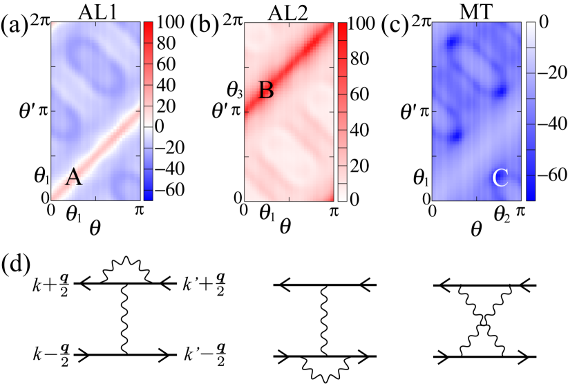
Figure S4: (a,b,c) $K_{\rm FS3}(\theta,\theta^{\prime})$ given by the AL1 term, the AL2 term, and the MT term, respectively. (d) Second-order diagrams with respect to ${\hat{\chi}}(q)$ except for the AL terms.

Here, we explain why the AL terms dominate over the MT term near the magnetic criticality based on the spin fluctuation theories S-TPSC ; S-Scalapino ; S-Monthoux ; S-Moriya ; S-Kontani-rev . The dynamical spin susceptibility is approximately expressed as

$$\chi^{s}({{\bm{q}}},{\omega}_{l})=\frac{a\xi^{2}}{1+\xi^{2}({{\bm{q}}}-{{\bm{Q}}})^{2}+|{\omega}_{l}|/{\omega}_{\rm sf}}$$ (S8)

where $\xi$ is the magnetic correlation length. The relation $\xi^{2}\propto(T-T_{N})^{-1}$ in the paramagnetic state according to spin fluctuation theories. ${\omega}_{\rm sf}\propto\xi^{-2}$ is the energy scale of spin fluctuations. Now, we discuss the absolute value of kernel in DW equation (2) in the main text, $f\equiv|T\sum_{k^{\prime}}{\hat{K}}^{\bm{0}}(k,k^{\prime})|$, in the case of $\xi\gg 1$ and ${\omega}_{\rm sf}\ll 2\pi T$. When the kernel for ${{\bm{q}}}={\bm{0}}$ is given by the AL term, $f_{\rm AL}\sim\sum_{{\bm{p}}}\{\chi^{s}({{\bm{p}}},0)\}^{2}\sim\xi^{2}$ in two-dimensional systems at a fixed $T$. (The electron Green functions in the AL diagram also give important $T$-dependence as discussed in Refs. S-FeSe-Yamakawa ; S-FeSe-Onari .) When the kernel is given by the MT term, $f_{\rm MT}\sim\sum_{{\bm{p}}}\chi^{s}({{\bm{p}}},0)\sim\log\xi$. Therefore, the AL term dominates over the MT term when $\xi\gg 1$. In the same way, the second-order diagrams except for the AL terms, shown in Fig. S4 (d), are scaled as $(\log\xi)^{2}$. Therefore, the AL terms are the most important for $\xi\gg 1$. The significance of the AL terms near the magnetic criticality is verified by the functional-renormalization-group (fRG) study in Refs. S-Tsuchiizu-Cu ; S-Tsuchiizu-CDW ; S-Tsuchiizu-Ru1 .

When $U$ is small and the relation $V^{s}(q)=U+U\chi^{s}(q)U\sim U$ holds, the AL term is very small and impossible to stabilize the bond order. With increasing $U$, the AL term becomes large in the case that $\chi^{s}({{\bm{p}}},{\omega}_{l})$ strongly develops for ${{\bm{p}}}\sim{{\bm{Q}}}$ at low energies. In the present model for AFe₂As₂, moderate spin fluctuations (Stoner factor ${\alpha}_{S}\approx 0.93$) are requied for the AL-term driving nematic order, whereas much weaker spin fluctuations are enough for FeSe as discussed in Refs. S-FeSe-Yamakawa ; S-FeSe-Onari .

I.5 E: Origin of $B_{1g}$ symmetry orbital order in undoped compounds

Here, we briefly explain the reason why ${B_{1g}}$ symmetry orbital order ($n_{xz}\neq n_{yz}$) appears in usual undoped ($n_{d}=6$) Fe-based superconductors. Figure S5 shows a simplified FSs, in which only $d_{xz}$ and $d_{yz}$ orbitals are shown. Here, spin fluctuations on $d_{xz[yz]}$-orbital develop at wavevector ${{\bm{Q}}}=(0,\pi)\ [(\pi,0)]$, due to the good intra-orbital FS nesting.

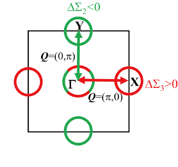
Figure S5: Simplified FSs for $n_{d}\approx 6$ composed of only $d_{xz}$ and $d_{yz}$ orbitals. Due to the intra-orbital FS nesting, spin fluctuations on $d_{xz}$ [$d_{yz}$] orbital develop at ${{\bm{Q}}}=(0,\pi)\ [{{\bm{Q}}}=(\pi,0)]$. These spin fluctuations induce nematic orbital order ($n_{xz}\neq n_{yz}$) cooperatively.

Here, we consider the DW equation (2) at ${{\bm{q}}}=\bm{0}$. In the kernel for $d_{yz}$ orbital, $K_{3,3;3,3}^{\bm{0}}({{\bm{k}}},{{\bm{k}}}^{\prime})$, the AL terms give large positive value for ${{\bm{k}}},{{\bm{k}}}^{\prime}\approx{{\bm{k}}}_{X}$ or ${{\bm{k}}}_{\Gamma}$. In contrast, the MT term give negative contribution for ${{\bm{k}}}\approx{{\bm{k}}}_{X}$ and ${{\bm{k}}}^{\prime}\approx{{\bm{k}}}_{\Gamma}$. Therefore, the form factor $\Delta\Sigma^{\bm{0}}_{3,3}({{\bm{k}}})$ takes large value in magnitude for ${{\bm{k}}}\approx{{\bm{k}}}_{X},{{\bm{k}}}_{\Gamma}$. ($\Sigma^{\bm{0}}_{3,3}({{\bm{k}}})|$ may have sign reversal between $\Gamma$ and $X$ points due to the MT term.) In the same way, $|\Delta\Sigma^{\bm{0}}_{2,2}({{\bm{k}}})|$ takes large value for ${{\bm{k}}}\approx{{\bm{k}}}_{Y},{{\bm{k}}}_{\Gamma}$.

In the Hubbard model, the net charge density (=charge monopole) order is strongly suppressed by the on-site Coulomb interaction $U$. In contrast, both the orbital order and the bond order can appear since they are (non-local) charge quadrupole orders. For this reason, the relation $\Delta\Sigma^{\bm{0}}_{2,2}(k_{x},k_{y})=-\Delta\Sigma^{\bm{0}}_{3,3}(k_{y},k_{x})$ is satisfied by solving the DW equation (2). This solution gives the orbital order ($n_{xz}\neq n_{yz}$) without net charge density modulation. Thus, spin fluctuations on $d_{xz}$ and $d_{yz}$ orbitals induce the orbital order ($n_{xz}\neq n_{yz}$) cooperatively. More detailed explanation is given in Refs. S-FeSe-Yamakawa ; S-FeSe-Onari .

Thus, the present study reveals the significant roles of FS orbital character and FS topology on the nature of nematicity. In usual compounds ($n_{d}\sim 6$) with FSs in Fig. S5, spin fluctuations on ($d_{xz},d_{yz}$) orbitals strongly develop. In this case, the nematic orbital order naturally appears. In heavily hole-doped compounds ($n_{d}\sim 5.5$), spin fluctuations develop solely in $d_{xy}$ orbital. Even in this case, nematic transition can appear by forming the bond order spontaneously as we revealed in the main text. We comment that the symmetry of nematicity is not simply related to the direction of wavevector of spin fluctuations. In summary, the diverse nematicity in Fe-based superconductors (such as $B_{1g}$ orbital order and $B_{2g}$ bond order) originates from the rich compound dependence of FS orbital character and FS topology.

I.6 F: Conserving approximation

In the main text, the self-energy correction is not included in the kernel function $K$. For this reason, the DW equation in the main text does not satisfy the condition of the conserving approximation (CA) formulated by Baym and Kadanoff. The great merit of the CA is that the macroscopic conservation laws are satisfied rigorously. This merit is important to avoid unphysical results. Here, we first calculate the one-loop self-energy using the fluctuation exchange (FLEX) approximation S-FLEX ; S-Onari-form . Next, we analyze the DW equation with including the FLEX self-energy, in order to satisfy the criteria of the CA.

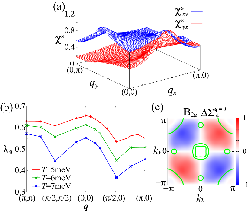
Figure S6: (a) ${{\bm{q}}}$ dependences of $\chi^{s}_{xy}({{\bm{q}}},0)$ and $\chi^{s}_{yz}({{\bm{q}}},0)$ given by the FLEX approximation. (b) $\bm{q}$ dependences of the maximum eigenvalue obtained by the present improved linearized DW equation. (c) Obtained form factors at ${{\bm{q}}}={\bm{0}}$ with ${B_{2g}}$ symmetry.

The FLEX self-energy (with $C_{4}$ symmetry) is given by $\hat{\Sigma}(k)=\frac{T}{N}\sum_{q}\hat{V}^{\Sigma}(q)\hat{G}(k-q)$, where ${\hat{G}}(k)=[(i{\epsilon}_{n}-\mu){\hat{1}}-{\hat{h}}^{0}({{\bm{k}}})-\hat{\Sigma}(k)]^{-1}$ is the Green function with the self-energy, and $\hat{V}^{\Sigma}$ given as $\displaystyle\frac{3}{2}{\hat{\Gamma}}^{s}{\hat{\chi}^{s}}(q){\hat{\Gamma}}^{s}+\frac{1}{2}{\hat{\Gamma}}^{c}{\hat{\chi}^{c}}(q){\hat{\Gamma}}^{c}-\frac{1}{2}\bigl{[}{\hat{\Gamma}}^{c}{\hat{\chi}}^{0}(q){\hat{\Gamma}}^{c}+{\hat{\Gamma}}^{s}{\hat{\chi}}^{0}(q){\hat{\Gamma}}^{s}-\frac{1}{4}({\hat{\Gamma}}^{s}+{\hat{\Gamma}}^{c}){\hat{\chi}}^{0}(q)({\hat{\Gamma}}^{s}+{\hat{\Gamma}}^{c})\bigr{]}$. We solve $\hat{\Sigma}$, $\hat{G}$, and $\hat{\chi}^{s(c)}$ self-consistently. Figure S6 (a) shows the ${{\bm{q}}}$-dependence of $\chi^{s}_{xy(yz)}$ given by the FLEX approximation for $T=5\sim 7$meV at fixed $r=0.96$ (${\alpha}_{S}=0.93$ at $T=5$meV) by employing $N=100\times 100$ ${{\bm{k}}}$-meshes. The obtained ${{\bm{q}}}$-dependence of $\chi^{s}_{xy(yz)}$ in the FLEX approximation is similar to that given by the RPA in the main text.

Next, we construct the improved DW equation to satisfy the framework of the CA, by introducing the obtained $\hat{\Sigma}$ and ${\hat{\chi}}^{s,c}$ into Eqs. (2)-(3) in the main text. Figure S6 (b) shows the eigenvalue $\lambda_{{{\bm{q}}}}$ given by solving the improved DW equation. It is confirmed that $\lambda_{{{\bm{q}}}}$ shows the maximum at ${{\bm{q}}}=\bm{0}$ for $T=5$meV($\lambda_{\bm{0}}=0.66$), consistently with the result without the self-energy in Fig. 2 (d). The obtained form factor $\Delta\Sigma_{4}^{\bm{0}}$ has ${B_{2g}}$ symmetry as shown in Fig. S6 (c), which is similar to Fig. 2 (a) in the main text. Thus, the results in the main text are verified by the present improved DW equation that satisfies the condition of the CA. The magnitude of $\lambda_{{{\bm{q}}}}$ is suppressed by including the self-energy. Although we cannot calculate for $T<5$meV due to the lack of frequency- and ${{\bm{k}}}$-mesh numbers, the value of $\lambda_{{{\bm{q}}}}$ will reach unity at lower temperature.

References

- (1) Y. Yamakawa, S. Onari and H. Kontani, Phys. Rev. X 6, 021032 (2016).
- (2) S. Onari, Y. Yamakawa, and H. Kontani, Phys. Rev. Lett. 116, 227001 (2016).
- (3) T. Miyake, K. Nakamura, R. Arita, and M. Imada, J. Phys. Soc. Jpn. 79, 044705 (2010).
- (4) D. Senechal and A.-M.S. Tremblay, Phys. Rev. Lett. 92, 126401 (2004).
- (5) P. Monthoux and D. J. Scalapino, Phys. Rev. Lett. 72, 1874 (1994).
- (6) P. Monthoux, D. Pines, and G. G. Lonzarich, Nature 450, 1177 (2007).
- (7) T. Moriya and K. Ueda, Adv. Phys. 49, 555 (2000).
- (8) H. Kontani, Rep. Prog. Phys. 71, 026501 (2008).
- (9) M. Tsuchiizu, K. Kawaguchi, Y. Yamakawa, and H. Kontani, Phys. Rev. B 97, 165131 (2018).
- (10) M. Tsuchiizu, Y. Yamakawa and H. Kontani, Phys. Rev. B 93, 155148 (2016).
- (11) M. Tsuchiizu, Y. Ohno, S. Onari, and H. Kontani, Phys. Rev. Lett. 111, 057003 (2013).
- (12) N. E. Bickers and S. R. White, Phys. Rev. B 43, 8044 (1991).
- (13) S. Onari, Y. Yamakawa, and H. Kontani, Phys. Rev. Lett. 116, 227001 (2016).