The distribution of Weierstrass points on a tropical curve

Abstract.

We show that on a metric graph of genus $g$, a divisor of degree $n$ generically has $g(n-g+1)$ Weierstrass points. For a sequence of generic divisors on a metric graph whose degrees grow to infinity, we show that the associated Weierstrass points become distributed according to the Zhang canonical measure. This distribution result has an analogue for complex algebraic curves, due to Neeman, and for curves over non-Archimedean fields, due to Amini. However, the results in this paper are purely combinatorial statements which are proved using elementary combinatorial arguments. No algebraic or analytic geometry is needed.

1. Introduction

To any divisor class on an algebraic curve, there is an associated set of Weierstrass points. In this paper we study the set of Weierstrass points associated to a divisor class on an abstract tropical curve. In particular, we ask

(A) When is the set of Weierstrass points finite? If so, how many are there?

and

(B) How are these points distributed as the degree approaches infinity?

We show that, for any abstract tropical curve $\Gamma$, the Weierstrass locus is finite for a generic divisor class. Generically, the number of Weierstrass points depends only on the degree of the divisor and the genus of the underlying curve. We further prove that, for any degree-increasing sequence of such generic divisors, the Weierstrass points become distributed according to the Zhang canonical measure on $\Gamma$. This measure can be described via interpreting $\Gamma$ as an electrical network of resistors.

We also define a stable Weiertrass locus which is finite for an arbitrary divisor class, and compute its cardinality for a generic divisor class, which depends only on the degree and genus.

1.1. Statement of results

Given a compact, connected metric graph $\Gamma$ and a divisor $D$ of rank $r=r(D)$, we define the Weierstrass locus ${W(D)}$ as

$$W(D)=\{x\in\Gamma:D\sim(r+1)x+E\text{ for some }E\geq 0\},$$

where $\sim$ denotes linear equivalence and $r(D)$ is the Baker–Norine rank (see Section 2 for definitions). The set $W(D)$ may fail to be finite; in some cases it contains all of $\Gamma$ (see Example 4.6).

For a divisor of degree $n\geq g$, we define the stable Weierstrass locus of $D$ as

$$W^{\mathrm{st}}(D)=\{x\in\Gamma:\operatorname{br}[D-(n-g)x]=x+E\text{ for some }E\geq 0\}$$

where $\operatorname{br}[D]$ denotes the unique break divisor representative of a degree $g$ divisor $D$. The stable Weierstrass locus is finite for any divisor. If $D$ has rank $r(D)=n-g$, i.e. $D$ is nonspecial, then the stable Weierstrass locus is contained in $W(D)$. In particular, this containment holds when the degree $n\geq 2g-1$. See Section 2 for definitions of linear equivalence, rank, and break divisor.

Our first result addresses the question of counting the number of Weierstrass points. Here “generic” means on a dense open subset of the space of divisor classes.

Theorem A.

Let $\Gamma$ be a compact, connected metric graph of genus $g$.

1. For a generic divisor class of degree $n\geq g$, the Weierstrass locus $W(D)$ is finite with cardinality

   $$\#W(D)=g(n-g+1).$$

   For a generic divisor class of degree $n<g$, $W(D)$ is empty.

2. For an arbitrary divisor class of degree $n\geq g$, the stable Weierstrass locus $W^{\mathrm{st}}(D)$ is a finite set with cardinality

   $$\#W^{\mathrm{st}}(D)\leq g(n-g+1),$$

   and equality holds for a generic divisor class.

Parts (a) and (b) of Theorem A are connected by showing that $W(D)=W^{\mathrm{st}}(D)$ for a generic divisor class.

The next main theorem of our paper describes the distribution of tropical Weierstrass points. Here, note that the condition “$W_{n}=W(D_{n})$ is a finite set” is satisfied for generic $[D_{n}]\in\operatorname{Pic}^{n}(\Gamma)$ by Theorem A.

Theorem B.

Let $\Gamma$ be a metric graph of genus $g$, and let $\{D_{n}:n\geq 1\}$ be a sequence of divisors on $\Gamma$ with $\deg D_{n}=n$. Let $W_{n}$ be the Weierstrass locus of $D_{n}$. Suppose each $W_{n}$ is a finite set, and let

$$\delta_{n}=\frac{1}{n}\sum_{x\in W_{n}}\delta_{x}$$

denote the normalized discrete measure on $\Gamma$ associated to $W_{n}$ (where $\delta_{x}$ is the Dirac measure at $x$). Then as $n\to\infty$, the measures $\delta_{n}$ converge weakly to the Zhang canonical measure $\mu$ on $\Gamma$.

The Zhang canonical measure is defined in Section 3. (Warning: we use a different normalization for $\mu$ than previous authors; namely we have total measure $\mu(\Gamma)=g$ rather than $\mu(\Gamma)=1$.) We also obtain a quantitative version of this distribution result which specifies a bound on the rate of convergence.

Theorem C.

Let $\Gamma$ be a metric graph of genus $g$, let $D_{n}$ be a divisor of degree degree $n>g$, and let $W_{n}=W(D_{n})$ denote the Weierstrass locus. Suppose $W_{n}$ is finite. Let $\mu$ denote the Zhang canonical measure on $\Gamma$.

1. For any segment $e$ in $\Gamma$,

   $$n\mu(e)-2g\leq\#(W_{n}\cap e)\leq n\mu(e)+g+2.$$

2. If $e$ is a segment of $\Gamma$ with $\mu(e)>\frac{2g}{n}$, then $e$ contains at least one Weierstrass point of $D_{n}$.

3. For a fixed continuous function $f:\Gamma\to\mathbb{R}$, as $n\to\infty$

   $$\frac{1}{n}\sum_{x\in W_{n}}f(x)=\int_{\Gamma}f(x)\mu(dx)+O\left(\frac{1}{n}\right).$$

   (The big-$O$ constant depends on $f$, but is independent of the divisors $D_{n}$.)

It is likely that the bounds in part (a) can be improved.

1.2. Previous work

The set of ordinary Weierstrass points on a complex algebraic curve of genus $g\geq 2$ has been a classical object of study (see e.g. [20]). This is a set of $g^{3}-g$ points (counting with multiplicity) on $X$ which are instrinsic to $X$ as an abstract curve, without reference to any (non-canonical) embedding of $X$ into an ambient space. They form a useful tool, e.g. for proving that the automorphism group of such a curve is finite. This notion naturally extends to higher Weierstrass points (or higher-order Weierstrass points), which is a finite set of points on $X$ associated to a choice of divisor class on $X$. The number of higher Weierstrass points (counted with multiplicity) grows quadratically as a function of the degree of $[D]$. In this paper, we focus on this more general notion of higher Weierstrass points. We refer to higher Weierstrass points of $D$ simply as Weierstrass points of $D$.

The following useful intution is given by Mumford [21]: the Weierstrass points associated to a divisor of degree $n$ form a higher-genus analogue of the set of $n$-torsion points on an elliptic curve. (Just as choosing a different origin for the group law on a genus $1$ curve leads to a different set of torsion points, choosing different degree $n$ divisors will give you different sets of Weierstrass points.) The fact that $n$-torsion points on a complex elliptic curve become “evenly distributed” as $n$ grows large leads one to ask whether the same phenomenon holds for Weierstrass points on other curves.

An answer was given by Neeman [22], who showed that for any complex curve (i.e. Riemann surface) of genus $g\geq 2$, when $n\to\infty$ the Weierstrass points of degree $n$ divisors become distributed according to the Bergman measure.

Theorem 1.1 (Neeman [22]).

Let $X$ be a compact Riemann surface of genus $g\geq 2$, and let $\{D_{n}:n\geq 1\}$ be a sequence of divisors on $X$ with $\deg D_{n}=n$. Let $W_{n}$ denote the Weierstrass locus of the divisor $D_{n}$, and let $\delta_{n}=\frac{1}{gn^{2}}\sum_{x\in W_{n}}\delta_{x}$ denote the normalized discrete measure on $X$ associated to $W_{n}$ (where $\delta_{x}$ is the Dirac measure at $x$). Then as $n\to\infty$, the measures $\delta_{n}$ converge weakly to the Bergman measure on $X$.

Before Neeman’s result, Olsen [23] showed that given a positive-degree divisor $D$ on a complex algebraic curve $X$, the union of the Weierstrass points of the multiples $nD$, over all $n\geq 1$, is dense in $X$ in the complex topology.

If one replaces the ground field $\mathbb{C}$ with a non-Archimedean field, one may consider the same question of how Weierstrass points are distributed inside the Berkovich analytification $X^{\text{an}}$ of an algebraic curve, say after retracting to a compact skeleton $\Gamma$. This was addressed by Amini in [2]. Here the Weierstrass points are distributed according to the Zhang canonical admissable measure, constructed by Zhang in [24].

Theorem 1.2 (Amini [2]).

Let $X$ be a smooth proper curve of genus $g\geq 1$ over a complete, algebraically closed, non-Archimedean field $K$ with non-trivial valuation and residue characteristic $0$. Let $\Gamma$ be a skeleton of the Berkovich analytification $X^{an}$ with retraction map $\rho:X^{an}\to\Gamma$. Let $D$ be a positive-degree divisor on $X(K)$. Let $W_{n}$ denote the Weierstrass locus of the divisor $nD$, and let $\delta_{n}=\frac{1}{\#W_{n}}\sum_{x\in W_{n}}\delta_{\rho(x)}$ denote the normalized discrete measure on $\Gamma$ associated to $W_{n}$ (where $\delta_{x}$ is the Dirac measure at $x$). Then as $n\to\infty$, the measures $\delta_{n}$ converge weakly to the Zhang canonical measure on $\Gamma$, up to a factor of $g$.

Zhang’s canonical measure does not have support on bridge edges, so it is indepedent of the choice of skeleton. Zhang’s construction was motivated by Arakelov’s pairing for divisors on a Riemann surface [4], for the purpose of answering questions in arithmetic geometry. Here we use a definition of $\mu$ along more elementary lines from Chinburg–Rumely [11] and Baker–Faber [6], using the notions of current flow and electric potential in a network of resistors.

In [2] Amini raises the question of whether the distribution of Weierstrass points is possibly intrisic to the metric graph $\Gamma$, without needing to identify $\Gamma$ with the skeleton of some Berkovich curve $X^{\text{an}}$. One major obstacle to this idea is that on a metric graph, the Weierstrass locus for a divisor may fail to be a finite set of points. Our approach is to sidestep this issue by showing that finiteness does hold for a generic choice of divisor class. With this assumption of genericity, we are able to show that distribution of Weierstrass points is intrinsic to $\Gamma$.

In [5], Baker studies ordinary Weierstrass points on graphs and on metric graphs, and mentions several applications of number theoric significance. These results are stated only for Weierstrass points assosicated to the canonical divisor; higher Weierstrass points for general divisors are not considered.

Technical note: our tropical curves $\Gamma$ have no “hidden genus” at vertices and no infinite legs, i.e. we restrict our attention to $X^{\text{an}}$ with totally degenerate reduction and no punctures.

1.3. Outline

In Section 2 we review background material on metric graphs and their divisor theory. In Section 3 we review the interpretation of a metric graph as an electrical resistor network, and define Zhang’s canonical measure. In Section 4 we define the Weierstrass locus and stable Weierstrass locus for a divisor on a metric graph, and give examples. In Section 5 we prove that $W(D)$ is generically finite and compute its cardinality (Theorem A). In Section 6, we prove results on the distribution of Weierstrass points on a metric graph (Theorems B and C).

1.4. Notation

Here we collect some notation which will be used throughout the paper.

$\Gamma$	a compact, connected metric graph
$\operatorname{PL}_{\mathbb{R}}(\Gamma)$	continuous, piecewise linear functions on $\Gamma$
$\operatorname{PL}_{\mathbb{Z}}(\Gamma)$	continous, piecewise $\mathbb{Z}$-linear functions on $\Gamma$
$\operatorname{S}(\Gamma)$	“well-behaved” piecewise smooth functions on $\Gamma$
$\operatorname{\Delta}(f)$	the principal divisor associated to a piecewise ($\mathbb{Z}$-)linear function $f$
$D$	a divisor on a metric graph or algebraic curve
$D_{n}$	a divisor of degree $n$
$K=K_{\Gamma}$	the canonical divisor on $\Gamma$
$r(D)$	the Baker–Norine rank of $D$
$\operatorname{Div}(\Gamma)$	divisors on $\Gamma$ (with $\mathbb{Z}$-coefficients)
$\operatorname{Div}_{\mathbb{R}}(\Gamma)$	divisors on $\Gamma$ with $\mathbb{R}$-coefficients, i.e. $\operatorname{Div}(\Gamma)\otimes_{\mathbb{Z}}\mathbb{R}$
$\operatorname{Div}^{d}(\Gamma)$	divisors of degree $d$ on $\Gamma$
$\operatorname{Pic}^{d}(\Gamma)$	divisor classes of degree $d$ on $\Gamma$
$\operatorname{Sym}^{d}(\Gamma)$	effective divisors of degree $d$ on $\Gamma$
$\operatorname{Eff}^{d}(\Gamma)$	effective divisor classes of degree $d$ on $\Gamma$
$[D]$	a divisor class; the set of divisors linearly equivalent to $D$
$|D|$	the space of effective divisors linearly equivalent to $D$
$\operatorname{red}_{x}[D]$	the $x$-reduced divisor equivalent to $D$, where $x\in\Gamma$
$\operatorname{br}[D]$	the break divisor equivalent to $D$, where $D$ has degree $g$
$\operatorname{Br}^{g}(\Gamma)$	the space of break divisors on $\Gamma$
$\mu=\mu_{\Gamma}$	the Zhang canonical measure on $\Gamma$
$G$	a finite, connected graph with vertex set $V(G)$ and edge set $E(G)$
$(G,\ell)$	a combinatorial model for a metric graph, where $\ell:E(G)\to\mathbb{R}_{\geq 0}$
$\mathcal{T}(G)$	the set of spanning trees of a graph $G$

2. Abstract tropical curves

In this section we define metric graphs and linear equivalence of divisors on metric graphs. We use the terms “metric graph” and “abstract tropical curve” interchageably. We recall the Baker–Norine rank of a divisor, and state the Riemann–Roch theorem which is satisfied by this rank function.

2.1. Metric graphs and divisors

A metric graph is a compact, connected metric space which comes from assigning positive real edge lengths to a finite connected combinatorial graph. Namely, we construct a metric graph $\Gamma$ by taking a finite set of edges $E=\{e_{i}\}$, each isometric to a real interval $e_{i}=[0,L_{i}]$ of length $L_{i}>0$, gluing their endpoints to a finite set of vertices $V$, and imposing the path metric. The underlying combinatorial graph $G=(E,V)$ is called a combinatorial model for $\Gamma$. We allow loops and parallel edges in a combinatorial graph $G$. We say $e$ is a segment of $\Gamma$ if it is an edge in some combinatorial model.

The valence $\operatorname{val}(x)$ of a point $x$ on a metric graph $\Gamma$ is defined to be the number on connected components of a sufficiently small punctured neighborhood of $x$. Points in the interior of a segment of $\Gamma$ always have valence 2. All points $x$ with $\operatorname{val}(x)\neq 2$ are contained in the vertex set of any combinatorial model.

The genus of a metric graph $\Gamma$ is its first Betti number as a topological space,

$$g(\Gamma)=b_{1}(\Gamma)=\dim_{\mathbb{R}}H_{1}(\Gamma,\mathbb{R}).$$

If $G$ is a combinatorial model for $\Gamma$, the genus is equal to $g(\Gamma)=\#E(G)-\#V(G)+1$.

Example 2.1.

The metric graph in Figure 1 has genus 0. A minimal combinatorial model has $8$ vertices and $7$ edges.

Figure 1. Metric graph of genus $0$.

Example 2.2.

The metric graph in Figure 2 has genus $2$. A minimal combinatorial model has $2$ vertices and $3$ edges.

Figure 2. Metric graph of genus $2$.

A divisor on a metric graph $\Gamma$ is a finite formal sum of points of $\Gamma$ with integer coefficients. The degree of a divisor is the sum of its coefficients; i.e. for the divisor $D=\sum_{x\in\Gamma}a_{x}x$, we have ${\deg(D)=\sum_{x\in\Gamma}a_{x}}$. We let $\operatorname{Div}(\Gamma)$ denote the set of all divisors on $\Gamma$, and let $\operatorname{Div}^{d}(\Gamma)$ denote the divisors of degree $d$. We say a divisor is effective if all of its coefficients are non-negative; we write $D\geq 0$ to indicate that $D$ is effective. More generally, we write $D\geq E$ to indicate that $D-E$ is an effective divisor. We let $\operatorname{Sym}^{d}(\Gamma)$ denote the set of effective divisors of degree $d$ on $\Gamma$. $\operatorname{Sym}^{d}(\Gamma)$ inherits from $\Gamma$ the structure of a polyhedral cell complex of dimension $d$.

We let $\operatorname{Div}_{\mathbb{R}}(\Gamma)$ denote the set of divisors on $\Gamma$ with coefficients in $\mathbb{R}$. In other words, $\operatorname{Div}_{\mathbb{R}}(\Gamma)=\operatorname{Div}(\Gamma)\otimes_{\mathbb{Z}}\mathbb{R}$.

2.2. Principal divisors and linear equivalence

We define linear equivalence for divisors on metric graphs, following Gathmann–Kerber [13] and Mikhalkin–Zharkov [19]. This notion is analogous to linear equivalence of divisors on an algebraic curve, where rational functions are replaced with piecewise $\mathbb{Z}$-linear functions.

A piecewise linear function on $\Gamma$ is a continuous function $f:\Gamma\to\mathbb{R}$ such that there is some combinatorial model for $\Gamma$ such that $f$ restricted to each edge is a linear function, i.e. a function of the form

$$f(x)=ax+b,\qquad a,b\in\mathbb{R},$$

where $x$ is a length-preserving parameter on the edge. We let $\operatorname{PL}_{\mathbb{R}}(\Gamma)$ denote the set of all piecewise linear functions on $\Gamma$.

A piecewise $\mathbb{Z}$-linear function on $\Gamma$ is a piecewise linear function such that all its slopes are integers, i.e. $f$ restricted to each edge has the form

$$f(x)=ax+b,\qquad a\in\mathbb{Z},\,b\in\mathbb{R}$$

(for some combinatorial model). We let $\operatorname{PL}_{\mathbb{Z}}(\Gamma)$ denote the set of all piecewise $\mathbb{Z}$-linear functions on $\Gamma$. The functions $\operatorname{PL}_{\mathbb{Z}}(\Gamma)$ are closed under the operations of addition, multiplication by $\mathbb{Z}$, and taking pairwise $\max$ and $\min$.

We let $UT_{x}\Gamma$ denote the unit tangent fan of $\Gamma$ at $x$, which is the set of “directions going away from $x$” on $\Gamma$. For $v\in UT_{x}\Gamma$, the symbol $\epsilon v$ for sufficiently small $\epsilon\geq 0$ means the point in $\Gamma$ that is distance $\epsilon$ away from $x$ in the direction $v$. For $v\in UT_{x}\Gamma$ and a function $f:\Gamma\to\mathbb{R}$ we let

$$D_{v}f(x)=\lim_{\epsilon\to 0^{+}}\frac{f(x+\epsilon v)-f(x)}{\epsilon}$$

denote the slope of $f$ while travelling away from $x$ in the direction $v$ (if it exists).

Given $f\in\operatorname{PL}_{\mathbb{Z}}(\Gamma)$, we define the principal divisor $\operatorname{\Delta}(f)\in\operatorname{Div}^{0}(\Gamma)$ by

$$\operatorname{\Delta}(f)=\sum_{x\in\Gamma}a_{x}x\qquad\text{where}\qquad a_{x}=\sum_{v\in UT_{x}\Gamma}D_{v}f(x).$$

In words, the coefficient in $\operatorname{\Delta}(f)$ of a point $x$ is equal to the sum of the outgoing slopes of $f$ at $x$. On a given segment, this divisor is supported on the finite set of points at which $f$ is not linear, sometimes called the “break locus” of $f$. If $\operatorname{\Delta}(f)=D-E$ where $D,E$ are effective divisors with disjoint support, then we call $D=\operatorname{\operatorname{\Delta}^{+}}(f)$ the divisor of zeros of $f$ and $E=\operatorname{\operatorname{\Delta}^{--}}(f)$ the divisor of poles of $f$.

We say two divisors $D,E$ are linearly equivalent, denoted $D\sim E$, if there exists a piecewise $\mathbb{Z}$-linear function $f$ such that

$$\operatorname{\Delta}(f)=D-E.$$

Note that linearly equivalent divisors must have the same degree. We let $[D]$ denote the linear equivalence class of divisor $D$, i.e.

$$[D]=\{E\in\operatorname{Div}(\Gamma):E\sim D\}=\{D+\operatorname{\Delta}(f):f\in\operatorname{PL}_{\mathbb{Z}}(\Gamma)\}.$$

We say a divisor class $[D]$ is effective, or write $[D]\geq 0$, if there is an effective representative ${E\sim D},\,E\geq 0$ in the equivalence class.

We let $|D|$ denote the (complete) linear system of $D$, which is the set of effective divisors linearly equivalent to $D$. We have

$$|D| =\{E\in\operatorname{Div}(\Gamma):E\sim D,\,E\geq 0\}$$

$$=\{D+\operatorname{\Delta}(f):f\in\operatorname{PL}_{\mathbb{Z}}(\Gamma),\,\operatorname{\Delta}(f)\geq-D\}.$$

Unlike $[D]$, the linear system $|D|$ is naturally a compact polyhedral complex, with topology induced by the inclusion $|D|\subset\operatorname{Sym}^{d}(\Gamma)$.

Remark 2.3 (Linear equivalence as chip firing).

We sometimes speak of a degree $n$ effective divisor on $\Gamma$ as a collection of $n$ “chips” placed on $\Gamma$. Changing the divisor $D$ to a linearly equivalent divisor $D^{\prime}$ can be achieved through a sequence of “chip firing moves” where we choose and elementary cut of $\Gamma$ consisting of $m$ segments of length $\epsilon$, and on each edge move a chip from one end to the other.

Figure 3. Chip firing across an elementary cut.

The piecewise-linear function associated to such a chip firing move has slope $0$ outside the cut segments, and slope $1$ on the cut segments. For more discussion see [3, Remark 2.2], [8, Section 1.5] and the references therein.

Remark 2.4 (Linear interpolation along $f$).

Given a function $f\in\operatorname{PL}_{\mathbb{Z}}(\Gamma)$, we may associate to $f$ a 1-parameter family of effective divisors which “linearly interpolate” between the zeros $\operatorname{\operatorname{\Delta}^{+}}(f)$ and poles $\operatorname{\operatorname{\Delta}^{--}}(f)$. We can think of this contruction as specifying a unique “geodesic path” between any two points in the complete linear system $|D|$. This notion previously appeared in [18] under the name t-path.

Namely, for $\lambda\in\mathbb{R}$ we let $\lambda\in\operatorname{PL}_{\mathbb{Z}}(\Gamma)$ also denote the constant function on $\Gamma$ by abuse of notation, and we define the effective divisor ${f}^{-1}_{\operatorname{\Delta}}(\lambda)$ by

$${f}^{-1}_{\operatorname{\Delta}}(\lambda)=\operatorname{\operatorname{\Delta}^{--}}(f)+\operatorname{\Delta}(\max\{f,\lambda\}).$$

See Figure 4 for an illustration. Note that according to this definition, ${{f}^{-1}_{\operatorname{\Delta}}(\lambda)=\operatorname{\operatorname{\Delta}^{--}}(f)}$ for $\lambda$ sufficiently large and ${{f}^{-1}_{\operatorname{\Delta}}(\lambda)=\operatorname{\operatorname{\Delta}^{+}}(f)}$ for $\lambda$ sufficiently small. It is clear from definition that for any $\lambda$, ${f}^{-1}_{\operatorname{\Delta}}(\lambda)$ is linearly equivalent to $\operatorname{\operatorname{\Delta}^{+}}(f)$ and to $\operatorname{\operatorname{\Delta}^{--}}(f)$.

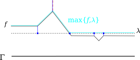
Figure 4. Linear interpolation showing the divisor ${f}^{-1}_{\operatorname{\Delta}}(\lambda)$.

2.3. Reduced divisors

A divisor class $[D]$ is typically very large, so it is convenient to have a method of choosing a (somewhat-)canonical representative divisor inside $[D]$. When $D$ has arbitrary degree, we can do so after fixing a basepoint $q$ on our metric graph $\Gamma$, using the $q$-reduced divisor construction.

Given a point $q\in\Gamma$, the $q$-reduced divisor $\operatorname{red}_{q}[D]$ is the unique divisor in $[D]$ which is effective away from $q$, and which minimizes a certain energy function among such representatives. Intuitively, $\operatorname{red}_{q}[D]$ is the divisor in $[D]$ whose chips are “as close as possible” to the basepoint $q$. We defer giving the full definition until Section 3.2, following [10, Appendix A]. For now, we state these important properties of the reduced divisor:

1. $[D]\geq 0$ if and only if $\operatorname{red}_{q}[D]\geq 0$

2. for any integer $m$, $\operatorname{red}_{q}[mq+D]=mq+\operatorname{red}_{q}[D]$

3. the degree of $\operatorname{red}_{q}[D]$ away from $q$ is at most $g$, the genus of $\Gamma$ (follows from Riemann’s inequality, Corollary 2.14)

4. for a fixed effective divisor $D$, the map $\Gamma\to|D|$ sending $q\mapsto\operatorname{red}_{q}[D]$ is continuous (due to Amini [1, Theorem 3]).

2.4. Break divisors and ABKS decomposition

When a divisor $D$ has degree $g$, there is a canonical representative of $[D]$ without any choice of basepoint, using the concept of break divisor. This notion was introduced by Mikhalkin–Zharkov [19] and studied extensively by An–Baker–Kuperberg–Shokrieh [3]. We review some of their results in this section.

A break divisor is an effective divisor of degree $g$ (the genus) which can be constructed in the following manner: choose a combinatorial model $G=(V,E)$ for $\Gamma$ and choose a spanning tree $T$ of $G$, then place one chip on each edge in the complement $E\backslash E(T)$. (Note that $E\backslash E(T)$ contains exactly $g$ edges.) Placing a chip on the endpoint of an edge is allowed.

The set of break divisors does not depend on the choice of combinatorial model. We use $\operatorname{Br}^{g}(\Gamma)$ to denote the set of all break divisors on $\Gamma$. We may view $\operatorname{Br}^{g}(\Gamma)$ as a topological space, using the topology induced from the inclusion in $\operatorname{Sym}^{g}(\Gamma)$.

Example 2.5.

In Figure 5 we show three examples of break divisors, on the left, and three examples of non-break divisors, on the right, on a genus $3$ metric graph.

Figure 5. Break divisors and non-break divisors

For a divisor class $[D]$ whose degree is $g$, the genus of the underlying curve, there is a unique representative of $[D]$ which is a break divisor.

Theorem 2.6 (see [3, Theorem 1.1], [19, Corollary 6.6]).

Let $\Gamma$ be a metric graph of genus $g$.

1. Every divisor class $[D]\in\operatorname{Pic}^{g}(\Gamma)$ contains a unique break divisor, which we denote $\operatorname{br}[D]$.

2. The map $\operatorname{br}:\operatorname{Pic}^{g}(\Gamma)\to\operatorname{Sym}^{g}(\Gamma)$ sending a divisor class to its break divisor representative is continuous and injective. Its image is the space of all break divisors $\operatorname{Br}^{g}(\Gamma)$.

3. The map $\operatorname{br}:\operatorname{Pic}^{g}(\Gamma)\to\operatorname{Sym}^{g}(\Gamma)$ is the unique continuous section of the map $[-]:\operatorname{Sym}^{g}(\Gamma)\to\operatorname{Pic}^{g}(\Gamma)$ taking an effective divisor to its linear equivalence class. Namely, $\operatorname{br}$ is the unique continuous map such that the composition

   $$\operatorname{Pic}^{g}(\Gamma)\xrightarrow{\operatorname{br}}\operatorname{Sym}^{g}(\Gamma)\xrightarrow{[-]}\operatorname{Pic}^{g}(\Gamma)$$

   is the identity homeomorphism.

If we choose a combinatorial model $(G,\ell)$ for the metric graph $\Gamma$, An–Baker–Kuperberg–Shokrieh [3] showed that the theory of break divisors implies a nice combinatorial decomposition of $\operatorname{Pic}^{g}(\Gamma)$. ($\operatorname{Pic}^{g}(\Gamma)$ is defined in Section 2.5.)

Theorem 2.7 (ABKS decomposition, see [3, Section 3.2]).

Suppose $\Gamma=(G,\ell)$ is a metric graph with a combinatorial model. Let $\mathcal{T}(G)$ denote the set of spanning trees of $G$. Then

$$\operatorname{Pic}^{g}(\Gamma)=\bigcup_{T\in\mathcal{T}(G)}C_{T}$$

where

$$C_{T}=\{[x_{1}+\cdots+x_{g}]:E(G)\backslash E(T)=\{e_{1},\ldots,e_{g}\},\,x_{i}\in e_{i}\}$$

denotes the set of divisor classes represented by summing a point from each edge of $G$ not in $T$. The cells $C_{T}$ have disjoint interiors, as $T\in\mathcal{T}(G)$ varies.

For fixed $T$, if we parametrize each edge $e_{i}\not\in E(T)$ as the closed real interval $[0,\ell(e_{i})]$, there is a natural surjective map $\prod_{i=1}^{g}[0,\ell(e_{i})]\to C_{T}$. This map always restricts to a homeomorphism on the respective interiors $\prod_{i=1}^{g}(0,\ell(e_{i}))\to C_{T}^{\circ}$, but may be non-injective on the boundary.

The proof is to combine Theorem 2.6 with the definition of break divisor, using the auxillary data of the spanning tree. Since $\operatorname{Pic}^{g}(\Gamma)$ is canonically homeomorphic to $\operatorname{Br}^{g}(\Gamma)$, we may view Theorem 2.7 as a decomposition of $\operatorname{Br}^{g}(\Gamma)$.

Remark 2.8.

If we take the combinatorial model for $\Gamma$ to be sufficiently subdivided, then for each $T=G\backslash\{e_{1},\ldots,e_{g}\}$, the surjection $\prod_{i=1}^{g}[0,\ell(e_{i})]\to C_{T}$ is a (global) homeomorphism. In particular, for this to hold it suffices that $G$ has girth $>g$ (i.e. every cycle contains more than $g$ edges). A necessary condition is that $G$ has no loops or parallel edges (if $g\geq 2$).

Example 2.9.

Consider the metric graph shown on the left side of Figure 6. Its minimial combinatorial model $\Gamma=(G,\ell)$ contains two vertices and three edges. The associated ABKS decomposition of $\operatorname{Pic}^{2}(\Gamma)$ is shown on the right side of Figure 6; segments on the boundary are glued to the parallel boundary segment. There are three cells, corresponding to the three spanning trees in $G$.

Here $\operatorname{Pic}^{2}(\Gamma)$ is homeomorphic to a torus (cf. Theorem 2.11). Each cell $C_{T}$ is homeomorphic to a rectangle with a pair of opposite vertices glued together.

Figure 6. ABKS decomposition of $\operatorname{Pic}^{2}(\Gamma)$.

Proposition 2.10.

Let $q\in\Gamma$ be an arbitrary basepoint on a genus $g$ metric graph.

1. For a generic divisor class $[D]$ of degree $g$, the reduced divisor $\operatorname{red}_{q}[D]$ is equal to the break divisor $\operatorname{br}[D]$.

2. For a generic divisor class $[D]$ of degree $n$, the reduced divisor $\operatorname{red}_{q}[D]$ is equal to

   $$\operatorname{red}_{q}[D]=(n-g)q+E$$

   where $E$ is a break divisor.

2.5. Picard group and Abel–Jacobi

We let $\operatorname{Pic}(\Gamma)$ denote the Picard group of $\Gamma$, which is the abelian group of all linear equivalence classes of divisors on $\Gamma$. The addition operation on $\operatorname{Pic}(\Gamma)$ is induced from addition of divisors in $\operatorname{Div}(\Gamma)$. In other words, $\operatorname{Pic}(\Gamma)$ is the cokernel of the map $\operatorname{\Delta}$ sending a piecewise $\mathbb{Z}$-linear function to its associated principal divisor:

$$\operatorname{PL}_{\mathbb{Z}}(\Gamma)\xrightarrow{\operatorname{\Delta}}\operatorname{Div}(\Gamma)\to\operatorname{Pic}(\Gamma)\to 0.$$

The kernel of $\operatorname{\Delta}$ is the set of constant functions on $\Gamma$.

Since the degree of a divisor class is well-defined, we have a disjoint union decomposition

$$\operatorname{Pic}(\Gamma)=\bigsqcup_{d\in\mathbb{Z}}\operatorname{Pic}^{d}(\Gamma).$$

The degree-0 component $\operatorname{Pic}^{0}(\Gamma)$ is a compact abelian group, and each $\operatorname{Pic}^{d}(\Gamma)$ is a torsor for $\operatorname{Pic}^{0}(\Gamma)$.

Theorem 2.11 (Abel–Jacobi for metric graphs).

Let $\Gamma$ be a metric graph of genus $g$. Then for any degree $d$, there is a homeomorphism of topological spaces

$$\operatorname{Pic}^{d}(\Gamma)\cong(S^{1})^{\times g}=\overbrace{S^{1}\times\cdots\times S^{1}}^{g}.$$

When $d=0$, this is an isomorphism of compact abelian topological groups.

Proof.

See Mikhalkin–Zharkov [19]. The proof follows the same idea as the classical Abel-Jacobi theorem, to show that $\operatorname{Pic}^{0}(\Gamma)=H^{1}(\Gamma,\mathbb{R})/H_{1}(\Gamma,\mathbb{Z})^{\vee}\cong\mathbb{R}^{g}/\mathbb{Z}^{g}$. ∎

We let $\operatorname{Eff}^{d}(\Gamma)$ denote the set of divisor classes on $\Gamma$ of degree $d$ which have an effective representative. In other words, $\operatorname{Eff}^{d}(\Gamma)$ is the image of $\operatorname{Sym}^{d}(\Gamma)$ under the (degree-$d$ restriction of the) cokernel map $\operatorname{Div}(\Gamma)\to\operatorname{Pic}(\Gamma)$:

The space $\operatorname{Eff}^{d}(\Gamma)$ is naturally a polyhedral complex of pure dimension $d$ when ${0\leq d\leq g}$ (see Gross et. al. [14]). As a particularly important case, the theta divisor $\Theta=\Theta(\Gamma)$ is $\Theta=\operatorname{Eff}^{g-1}(\Gamma)$, which lives inside $\operatorname{Pic}^{g-1}(\Gamma)$ as a codimension 1 polyhedral complex.

Remark 2.12.

The map $\operatorname{\Delta}:\operatorname{PL}_{\mathbb{Z}}(\Gamma)\to\operatorname{Div}(\Gamma)$ is also known as the metric graph Laplacian on $\Gamma$. This comes from identitying $\operatorname{Div}(\Gamma)$ with the space of integer-valued discrete measures on $\Gamma$, via

$$D=\sum_{i=1}^{n}a_{i}x_{i}\quad\longleftrightarrow\quad\delta=\sum_{i=1}^{n}a_{i}\delta_{x_{i}}$$

so that $\operatorname{\Delta}(f)$ coincides with the (distributional) second derivative $-\frac{d^{2}}{dx^{2}}f(x)$, at least for $x$ in the interior of an edge. The definition of metric graph Laplacian naturally extends to piecewise linear functions on $\Gamma$ with arbitrary real slopes, if we also allow real-valued coefficients in the divisor $\operatorname{\Delta}(f)$. This yields a map

$$\operatorname{PL}_{\mathbb{R}}(\Gamma)\xrightarrow{\operatorname{\Delta}}\operatorname{Div}_{\mathbb{R}}(\Gamma).$$

The cokernel of this map is less interesting (e.g. it does not tell us the genus of $\Gamma$); it is simply the degree function $\operatorname{Div}_{\mathbb{R}}(\Gamma)\xrightarrow{\text{deg}}\mathbb{R}$. We will see why this is the cokernel in Section 3.1 on voltage functions. This fits in the short exact sequence

$$0\to\mathbb{R}\xrightarrow{\text{const}}\operatorname{PL}_{\mathbb{R}}(\Gamma)\xrightarrow{\operatorname{\Delta}}\operatorname{Div}_{\mathbb{R}}(\Gamma)\xrightarrow{\text{deg}}\mathbb{R}\to 0.$$

(Compare to the integral case

$$0\to\mathbb{R}\xrightarrow{\text{const}}\operatorname{PL}_{\mathbb{Z}}(\Gamma)\xrightarrow{\operatorname{\Delta}}\operatorname{Div}(\Gamma)\xrightarrow{}\operatorname{Pic}(\Gamma)\to 0$$

where $\operatorname{Pic}(\Gamma)\cong\mathbb{Z}\times(S^{1})^{g}$.)

2.6. Rank and Riemann–Roch

We recall the definition of the rank of a divisor on a metric graph, which is due to Baker and Norine [8] (originally for divisors on a combinatorial graph) and extended to metric graphs by Gathmann–Kerber [13] and Mikhalkin–Zharkov [19]. The rank function is a natural way to extend the important distinction between effective and non-effective divisor classes on a metric graph. Divisor classes with larger rank are in a sense “further away” from the set of non-effective divisor classes, where distance between divisors is given by adding or subtracting single points.

The rank $r(D)$ of a divisor $D$ on $\Gamma$ is defined as

$$r(D)=\max\{r\geq 0:[D-E]\geq 0\text{ for all }E\in\operatorname{Sym}^{r}(\Gamma)\}$$

if $[D]$ is effective, and $r(D)=-1$ otherwise. Equivalently,

$$r(D)=\begin{cases}-1&\text{if $[D]$ is not effective},\\ 1+\displaystyle\min_{x\in\Gamma}\{r(D-x)\}&\text{if $[D]$ is effective}.\end{cases}$$

This second definition inductively gives the rank of a divisor in terms of divisors of smaller degree; the base case is the set of non-effective divisor classes. Note that the rank of a divisor $D$ depends only on its linear equivalence class.

The canonical divisor on a metric graph $\Gamma$ is defined as

$$K=\sum_{x\in\Gamma}(\operatorname{val}(x)-2)\cdot x.$$

The degree of the canonical divisor is $\deg K=2g-2$, which agrees with the canonical divisor on an algebraic curve.

Theorem 2.13 (Riemann-Roch for metric graphs).

Let $\Gamma$ be a metric graph of genus $g$, and let $K$ be the canonical divisor on $\Gamma$. For any divisor $D$ on $\Gamma$,

$$r(D)-r(K-D)=\deg(D)+1-g.$$

Proof.

See Gathmann–Kerber [13, Proposition 3.1] and Mikhalkin–Zharkov [19, Theorem 7.3], which both adapt the arguments of Baker–Norine [8] for the case of combinatorial graphs. ∎

Corollary 2.14 (Riemann’s inequality for metric graphs).

For a divisor $D$ on a metric graph of genus $g$,

$$r(D)\geq\deg(D)-g.$$

Proof.

This follows from Riemann–Roch since $r(K-D)\geq-1$. ∎

By Riemann’s inequality, any divisor $D$ satisfies $r(D)\geq\max\{\deg(D)-g,-1\}$. We say $D$ is nonspecial if this bound on $r(D)$ is achieved.

3. Canonical measure and resistor networks

In this section we define the Zhang canonical measure on a metric graph (due to Zhang [24]) via the perspective of resistor networks following Baker–Faber [6]. We may view this construction as a one-dimensional analogue of Gaussian curvature on a closed two-dimensional surface.

3.1. Voltage function

We view a metric graph $\Gamma$ as a resistor network by interpreting an edge of length $L$ as a resistor of resistance $L$. Note that this is well-defined on a metric graph due to the series rule for combining resistances, so we have compatibility with subdividing an edge into edges of shorter length. This interpretation is not only mathematically convenient, but physically honest—the electrical resistance of a wire is directly proportional to its length, a fact known as Pouillet’s law.

On a resistor network we may send current from one point to another. On a given segment, the voltage drop across the segment is equal to the resistance (i.e. length) of the segment multiplied by the amount of current passing through the segment—this is Ohm’s law. Under an externally-applied current, the flow of current within the network is determined by Kirchoff’s circuit laws: the current law says that the sum of directed currents out of any point is equal to zero (accounting for external currents), and the voltage law says that the sum of directed voltage differences around any closed loop is equal to zero. It is a well-known empirical fact that Kirchoff’s circuit laws can be solved uniquely for any externally-applied current flow which satisfies conservation of current (i.e. internal current flows are unique). To some, it is also a well-known mathematical result.

Our convention is that current flows from higher voltage to lower voltage.

Definition 3.1 (physics version).

Given points $y,z\in\Gamma$, the voltage function (or electric potential function) $j_{z}^{y}:\Gamma\to\mathbb{R}$ is defined by

$$j_{z}^{y}(x)=\text{voltage at $x$ when sending one unit of current from $y$ to $z$,}$$

such that $j_{z}^{y}(z)=0$, i.e. the network is “grounded” at $z$.

Definition 3.2 (math version; definition–theorem).

Given points $y,z\in\Gamma$, the voltage function $j_{z}^{y}$ is the unique function in $\operatorname{PL}_{\mathbb{R}}(\Gamma)$ satisfying the conditions

$$\operatorname{\Delta}(j_{z}^{y})=z-y\in\operatorname{Div}_{\mathbb{R}}^{0}(\Gamma)\quad\text{and}\quad j_{z}^{y}(z)=0.$$

Proof.

For the existence and uniqueness of $j_{z}^{y}$, see Theorem 6 and Corollary 3 of Baker–Faber [6]. Note that they use the notation $j_{z}(y,-)$ for $j_{z}^{y}(-)$. ∎

Note that $j_{z}^{y}$ satisfies the following properties:

1. for any $x\in\Gamma$, $0=j_{z}^{y}(z)\leq j_{z}^{y}(x)\leq j_{z}^{y}(y)$

2. $j_{z}^{y}(x)$ is piecewise linear in $x$

3. $j_{z}^{y}{(x)}$ is continuous in $x$, $y$, and $z$.

Proposition 3.3.

The voltage function $j_{z}^{y}$ obeys the following symmetries.

1. For any three points $x,y,z\in\Gamma$,

   $$j_{z}^{y}(x)=j_{z}^{x}(y)$$

2. For any four points $x,y,z,w\in\Gamma$,

   $$j_{z}^{y}(x)-j_{z}^{y}(w)=j_{w}^{x}(y)-j_{w}^{x}(z).$$

Proof.

See Baker–Faber [6, Theorem 8]; they refer to (b) as the “Magical Identity”. Note that (a) follows from (b) by setting $z=w$. ∎

Remark 3.4.

We many interpret any function $f\in\operatorname{PL}_{\mathbb{R}}(\Gamma)$ as a voltage function on $\Gamma$, which results from the externally applied current $\operatorname{\Delta}(f)\in\operatorname{Div}_{\mathbb{R}}(\Gamma)$. In other words, the voltage $f$ results from sending current from $\operatorname{\operatorname{\Delta}^{--}}(f)$ to $\operatorname{\operatorname{\Delta}^{+}}(f)$ in $\Gamma$.

The existence of $j_{z}^{y}\in\operatorname{PL}_{\mathbb{R}}(\Gamma)$ for any $y,z\in\Gamma$ implies that the principal divisor map $\operatorname{\Delta}:\operatorname{PL}_{\mathbb{R}}(\Gamma)\to\operatorname{Div}_{\mathbb{R}}^{0}(\Gamma)$ is surjective. This verifies the claim made in Remark 2.12 concerning the exactness of the sequence

$$0\to\mathbb{R}\xrightarrow{\text{const}}\operatorname{PL}_{\mathbb{R}}(\Gamma)\xrightarrow{\operatorname{\Delta}}\operatorname{Div}_{\mathbb{R}}(\Gamma)\xrightarrow{\text{deg}}\mathbb{R}\to 0.$$

Proposition 3.5 (Slope-current principle).

Suppose $f\in\operatorname{PL}_{\mathbb{R}}(\Gamma)$ has zeros $\operatorname{\operatorname{\Delta}^{+}}(f)$ and poles $\operatorname{\operatorname{\Delta}^{--}}(f)$ of degree $d\in\mathbb{R}$. Then the slope of $f$ is bounded by $d$, i.e.

$$|f^{\prime}(x)|\leq d\qquad\text{for any $x$ where $f$ is linear}.$$

(This bound is sharp; it is attained only on bridge edges, and only when all zeros are on one side of the bridge and all poles are on the other side.)

Proof.

Let $\lambda=f(x)$. Then the “tropical preimage”

$${f}^{-1}_{\operatorname{\Delta}}(\lambda):=\operatorname{\operatorname{\Delta}^{--}}(f)+\operatorname{\Delta}(\max\{f,\lambda\})$$

has multiplicity $|f^{\prime}(x)|$ at $x$, since the outgoing slopes of $\max\{f,\lambda\}$ at $x$ are $|f^{\prime}(x)|$ and $0$. (Note $x$ cannot be in $\operatorname{\operatorname{\Delta}^{--}}(f)$ since $f$ is linear at $x$.) Since the divisor ${f}^{-1}_{\operatorname{\Delta}}(\lambda)$ is effective of degree $d$, this implies $|f^{\prime}(x)|\leq d$ as desired. ∎

Remark 3.6.

The above proposition is obvious from its “physical interpretation”: $f$ gives the voltage in the resistor network $\Gamma$ when subjected to an external current described by $\operatorname{\operatorname{\Delta}^{--}}(f)$ units flowing into the network and $\operatorname{\operatorname{\Delta}^{+}}(f)$ units flowing out. The slope $|f^{\prime}(x)|$ is equal to the current flowing through the wire containing $x$, which must be no more than the total in-flowing (or out-flowing) current.

Next we address how the voltage function $j_{z}^{y}\in\operatorname{PL}_{\mathbb{R}}(\Gamma)$ may be approximated by a sequence of functions in $\operatorname{PL}_{\mathbb{Z}}(\Gamma)$ (up to rescaling), which depend on reduced divisors. (We only use property (RD3) of reduced divisors.)

Proposition 3.7 (Discrete approximation of voltage function).

Let $\{D_{n}:{n\geq 1}\}$ be a sequence of divisors on $\Gamma$ with $\deg D_{n}=n$. Fix two points $y,z\in\Gamma$. Let $\operatorname{red}_{y}[D_{n}]$ and $\operatorname{red}_{z}[D_{n}]$ denote the $y$– and $z$–reduced representatives in the divisor class $[D_{n}]$, and let $f_{n}$ be the unique function in $\operatorname{PL}_{\mathbb{Z}}(\Gamma)$ satisfying

$$\operatorname{\Delta}(f_{n})=\operatorname{red}_{z}[D_{n}]-\operatorname{red}_{y}[D_{n}]$$

and $f_{n}(z)=0$. Then the functions $\frac{1}{n}f_{n}$ converge uniformly to $j_{z}^{y}$ as $n\to\infty$.

Proof.

If the sequence $\frac{1}{n}h_{n}$ converges to a limit, then the sequence $\frac{1}{n+c}h_{n}$ must also converge to the same limit as $n\to\infty$, for any constant $c$. Thus it suffices to show that the functions $\frac{1}{n}f_{n+g}$ converge uniformly to $j_{z}^{y}$.

Let $\phi_{n}=\frac{1}{n}f_{(n+g)}-j_{z}^{y}$. We claim that the sequence of functions $\{\phi_{n}\in\operatorname{PL}_{\mathbb{R}}(\Gamma):n\geq 1\}$ converges uniformly to $0$. Note that each $\phi_{n}$ is a continuous, piecewise-differentiable function with $\phi_{n}(z)=0$, so for an arbitrary $x\in\Gamma$ we may calculate the value of $\phi_{n}(x)$ by integrating the derivative of $\phi_{n}$ along some path in $\Gamma$ from $z$ to $x$. The length of such a path is bounded uniformly in $x$, since $\Gamma$ is compact, so to show that $\phi_{n}\to 0$ uniformly it suffices to show that the magnitude of the derivative $|\phi_{n}^{\prime}|$ approaches $0$ uniformly.

Claim: For any $x\in\Gamma$, $|\phi_{n}^{\prime}(x)|\leq\frac{g}{n}$.

This follows from the slope-current principle (Proposition 3.5). By Riemann’s inequality, the $y$-reduced representative in $[D_{(n+g)}]$ may be expressed as

$$\operatorname{red}_{y}[D_{n+g}]=ny+E_{n}$$

for some effective divisor $E_{n}$ of degree $g$. Similary, $\operatorname{red}_{z}[D_{n+g}]=nz+F_{n}$ for some effective $F_{n}$ of degree $g$. Thus the principal divisor associated to $\frac{1}{n}f_{n+g}$ is

$$\operatorname{\Delta}(\frac{1}{n}f_{n+g})=z+\frac{1}{n}F_{n}-y-\frac{1}{n}E_{n}.$$

Recall that $\operatorname{\Delta}(j_{z}^{y})=z-y$; it follows that the principal $\mathbb{R}$-divisor associated to $\phi_{n}$ is

$$\operatorname{\Delta}(\phi_{n})=\operatorname{\Delta}\left(\frac{1}{n}f_{n+g}-j_{z}^{y}\right)=\frac{1}{n}F_{n}-\frac{1}{n}E_{n}.$$

In particular, $\operatorname{\Delta}(\phi_{n})$ is a difference of effective $\mathbb{R}$-divisors of degree $\frac{g}{n}$, so the zeros $\operatorname{\operatorname{\Delta}^{+}}(\phi_{n})$ and poles $\operatorname{\operatorname{\Delta}^{--}}(\phi_{n})$ each have degree at most $\frac{g}{n}$. By Proposition 3.5, this implies $|\phi_{n}^{\prime}(x)|\leq\frac{g}{n}$ as claimed. ∎

We separate the central claim in the above proof to a named proposition, for future reference.

Proposition 3.8 (Quantitative version of voltage approximation).

Let $\Gamma$ be a metric graph of genus $g$, and let $D_{n}$ be a degree $n$ divisor on $\Gamma$. Fix two points $y$ and $z$ on $\Gamma$, and let $f_{n}$ be the unique function in $\operatorname{PL}_{\mathbb{Z}}(\Gamma)$ satisfying

$$\operatorname{\Delta}(f_{n})=\operatorname{red}_{z}[D_{n}]-\operatorname{red}_{y}[D_{n}]$$

and $f_{n}(z)=0$. Then for $n>g$ and any $x\in\Gamma$, $|(\frac{1}{n-g}f_{n}-j_{z}^{y})^{\prime}(x)|\leq\frac{g}{n-g}$.

Remark 3.9.

We can interpret Proposition 3.7 as follows: the existence of the voltage function $j_{z}^{y}:\Gamma\to\mathbb{R}$ follows from Riemann’s inequality for divisors on $\Gamma$.

3.2. Energy and reduced divisors

Here we give a definition of $q$-reduced divisors on a metric graph. We will only need to use $q$-reduced divisors for effective divisor classes, so we restrict our discussion here to the effective case.

Definition 3.10.

Given a basepoint $q$ on $\Gamma$, we define the $q$-energy $\mathcal{E}_{q}:\Gamma\to\mathbb{R}$ by

$$\mathcal{E}_{q}(y)=j_{q}^{y}(y)=r(y,q).$$

Given an effective divisor $D=\sum_{i}y_{i}$, we define the $q$-energy $\mathcal{E}_{q}(D)$ by

$$\mathcal{E}_{q}(D)=\sum_{i}\sum_{j}j_{q}^{y_{i}}(y_{j}).$$

Note that

• $\mathcal{E}_{q}(D)\geq 0$,

• $\mathcal{E}_{q}(D)$ is strictly positive if $D$ has support outside of $q$,

• $\mathcal{E}_{q}(D)\geq\sum_{i}\mathcal{E}_{q}(y_{i})$, and in general this inequality is strict.

Theorem 3.11 (Baker–Shokrieh [10, Theorem A.7]).

Fix a basepoint $q\in\Gamma$, and let $D$ be an effective divisor on $\Gamma$. There is a unique divisor $D_{0}\in|D|$ which minimizes the $q$-energy, i.e. such that

$$\mathcal{E}_{q}(D_{0})<\mathcal{E}_{q}(E)\qquad\text{for all}\qquad E\in|D|,\,E\neq D_{0}.$$

Definition 3.12.

The $q$-reduced divisor $\operatorname{red}_{q}[D]$ is the unique divisor in $|D|$ which minimizes the $q$-energy $\mathcal{E}_{q}$.

Note that this definition is non-standard; the standard definition for reduced divisor is a combinatorial condition which can be phrased in the language of chip-firing, see [1, p. 4854], [3, Definition 2.3].

Example 3.13.

In Figure 7 we show a degree $4$ divisor, on the left, and its reduced representative with respect to basepoint $q$, on the right.

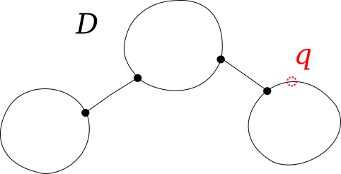
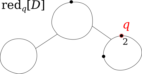
Figure 7. A divisor and its reduced divisor representative

3.3. Resistance function

In this section we recall the definition of the (Arakelov–Zhang–Baker–Faber) canonical measure $\mu$ on a metric graph.

Definition 3.14.

Let $r:\Gamma\times\Gamma\to\mathbb{R}$ denote the effective resistance function on the metric graph $\Gamma$. Namely, viewing $\Gamma$ as a resistor network

$$r(x,y) =\text{effective resistance between $x$ and $y$}$$

$$=\text{total voltage drop when sending 1 unit of current from $x$ to $y$}$$

If we wish to emphasize the underlying graph, we write $r(x,y;\Gamma)$.

In terms of the voltage function from Section 3.1, $r(x,y)=j_{y}^{x}(x)$.

It is straighforward to verify that the resistance function satisfies the following properties

1. $r(x,x)=0$,

2. $r(x,y)>0$ if $x\neq y$,

3. $r(x,y)$ is continuous with respect to $x$ and $y$

4. $r(x,y)=r(y,x)$

In contrast with the voltage function $j_{z}^{y}$, the function $x\mapsto r(x,y)$ is not piecewise linear. We will see that it is instead piecewise quadratic.

There is a special case of effective resistance which will be particularly useful in the following sections.

Definition 3.15.

Given a segment $e$ in a metric graph $\Gamma$, the deleted effective resistance $\ell_{\text{eff}}({\Gamma\backslash e})$ is the effective resistance between endpoints of $e$ in the $e$-deleted subgraph; that is, if $s,t$ are the endpoints of $e$

$$\ell_{\text{eff}}({\Gamma\backslash e})=r(s,t;\Gamma\backslash e).$$

Note that $\ell_{\text{eff}}({\Gamma\backslash e})=0$ when $e$ is a loop, and $\ell_{\text{eff}}({\Gamma\backslash e})=+\infty$ when $e$ is a bridge. The rule for combining resistances in parallel implies that for a segment $e$ with endpoints $s$ and $t$,

$$r(s,t;\Gamma)=\left(\frac{1}{\ell({e})}+\frac{1}{\ell_{\text{eff}}({\Gamma\backslash e})}\right)^{-1}=\frac{\ell({e})\ell_{\text{eff}}({\Gamma\backslash e})}{\ell({e})+\ell_{\text{eff}}({\Gamma\backslash e})}.$$

Example 3.16.

Let $\Gamma$ be a circle of circumference $L$. By choosing a basepoint which we denote as $0$, we may parametrize $\Gamma$ with the interval $[0,L]$. Identifying points in this way, we have

$$r(x,0) =\text{parallel combination of resistances $x$ and $L-x$}$$

$$=\frac{x(L-x)}{x+(L-x)}=x-\frac{1}{L}x^{2}.$$

The effective resistance is maximized when $x=\frac{1}{2}L$, with maximum value $\frac{1}{4}L$. The effective resistance is minimized when $x=0$ or $x=L$, with effective resistance $0$.

3.4. Canonical measure

Definition 3.17.

The canonical measure $\mu=\mu_{\Gamma}$ on a metric graph $\Gamma$ is the continuous measure defined by

$$\mu=\mu(dx)=-\frac{1}{2}\frac{d^{2}}{dx^{2}}r(x,y_{0})\,dx.$$

where $x$ is a length-preserving parameter on a segment, $dx$ is the Lebesgue measure, and $y_{0}$ is a fixed point in $\Gamma$. This defines $\mu$ on the open dense subset of $\Gamma$ where the second derivative exists; at the finite set of points where $r(-,y_{0})$ is not differentiable, or where the valence of $x$ differs from 2, we let $\mu_{\Gamma}=0$.

Remark 3.18.

The first derivative of a smooth function on $\Gamma$ is only well-defined up to a choice of sign, since there are two directions in which we could parametrize any segment. The second derivative, however, is well-defined on each segment (without choosing an orientation) because $(\pm 1)^{2}=1$ so either choice of direction yields the same second derivative.

Remark 3.19.

The definition of canonical measure is independent of the choice of basepoint $y_{0}$ because of the “Magical Identity” in Proposition 3.3 (b). Namely, for two basepoints $y_{0},z_{0}$ we have $j_{y_{0}}^{x}(x)-j_{y_{0}}^{x}(z_{0})=j_{z_{0}}^{x}(x)-j_{z_{0}}^{x}(y_{0})$ which implies

$$r(x,y_{0})-r(x,z_{0}) =j_{y_{0}}^{x}{(x)}-j_{z_{0}}^{x}{(x)}$$

$$=j_{y_{0}}^{x}(z_{0})-j_{z_{0}}^{x}(y_{0})=j_{y_{0}}^{z_{0}}(x)-j_{z_{0}}^{y_{0}}(x).$$

Since the voltage functions $j_{y_{0}}^{z_{0}},j_{z_{0}}^{y_{0}}$ are piecewise linear, we have

$$\frac{d^{2}}{dx^{2}}(r(x,y_{0})-r(x,z_{0}))=\frac{d^{2}}{dx^{2}}(j_{y_{0}}^{z_{0}}(x)-j_{z_{0}}^{y_{0}}(x))=0.$$

Remark 3.20.

The definition of canonical measure given here differs from that used by Baker–Faber [6], in that our $\mu$ does not have a discrete part supported at the points of $\Gamma$ with valence different from $2$.

Remark 3.21.

The definition of canonical measure given here is equal to Zhang’s canonical measure [24, Section 3, Theorem 3.2 c.f. Lemma 3.7] associated to the canonical divisor $D=K$, up to a multiplicative factor. Our canonical measure is normalized to satisfy $\mu(\Gamma)=g$ rather than $\mu(\Gamma)=1$.

The canonical measure of Baker–Faber is equal to Zhang’s canonical measure associated to $D=0$.

Example 3.22 (Canonical measure on cirlce).

If $\Gamma$ is a circle of circumference $L$, by Example 3.16 we have ${r(x,0)=x-\frac{1}{L}x^{2}}$ so the canonical measure is ${\mu=\frac{1}{L}dx}$. The total measure on the metric graph is $\mu(\Gamma)=1$.

Example 3.23 (Canonical measure on theta graph).

Consider the metric graph $\Gamma$ of genus 2 shown in Figure 8, with edge lengths $a,b,c$.

$\ell({e})=a$

$\ell_{\text{eff}}({\Gamma\backslash e})=\frac{bc}{b+c}$

Figure 8. Genus 2 metric graph with edge lengths $a,b,c$.

On the edge of length $a$, we have $\ell({e})=a$ and $\ell_{\text{eff}}({\Gamma\backslash e})=\frac{bc}{b+c}$. When measuring effective resistance between points in the interior of $e$, we can think of $\Gamma$ as a circle of total length $\ell({e})+\ell_{\text{eff}}({\Gamma\backslash e})=\frac{ab+ac+bc}{b+c}$. Thus the canonical measure on this edge is $\mu=\frac{b+c}{ab+ac+bc}dx$, by the computation for a circle in Example 3.16. The total measure on this edge is $\mu(e)=\frac{ab+ac}{ab+ac+bc}$, and by symmetry the total measure on the metric graph is $\mu(\Gamma)=2$.

Proposition 3.24.

The canonical measure $\mu$ on a metric graph $\Gamma$ is a piecewise-constant multiple of the Lebesgue measure which vanishes on all bridge segments.

On a non-bridge segment $e$ in $\Gamma$,

$$\mu|_{e}=\frac{1}{\ell({e})+\ell_{\text{eff}}({\Gamma\backslash e})}dx$$

where $\ell({e})$ denotes the length of $e$ and $\ell_{\text{eff}}({\Gamma\backslash e})$ denotes the effective resistance between the endpoints of $e$ on the graph after removing the interior of $e$.

For a bridge segment, $\mu|_{e}=0$.

Proof.

See Baker–Faber [6, Theorem 12]; note that our $\mu$ is defined to be the continuous part of Baker–Faber’s $\mu_{\text{can}}$.

(The proof idea should be clear from Example 3.23.) ∎

If a segment $e$ is subdivided into $e_{1}\sqcup e_{2}$, the expression $\mu|_{e}$ agrees with $\mu|_{e_{1}}=\mu|_{e_{2}}$.

Corollary 3.25.

Let $\Gamma$ be a metric graph with canonical measure $\mu$, and let $e$ be a segment in $\Gamma$ (i.e. $e$ is subspace isometric to a closed interval, whose interior points all have valence $2$ in $\Gamma$). Then

1. $0\leq\mu(e)\leq 1$;

2. $\mu(e)=0\quad\Leftrightarrow\quad$ $e$ is a bridge edge;

3. $\mu(e)=1\quad\Leftrightarrow\quad$ $e$ is a loop edge.

Proof.

By Proposition 3.24, $\mu(e)=0$ for bridges and $\mu(e)=\frac{\ell({e})}{\ell({e})+\ell_{\text{eff}}({\Gamma\backslash e})}$ otherwise. ∎

Proposition 3.26 (Foster’s theorem).

Let $\Gamma$ be a metric graph of genus $g$, and let $\mu$ be the canonical measure on $\Gamma$. Then the total measure on $\Gamma$ is

$$\mu(\Gamma)=g.$$

Proof.

See Baker–Faber [6, Corollary 5 and Corollary 6] and Foster [12]. ∎

4. Weierstrass points

In this section we define the Weierstrass locus and the stable Weierstrass locus of an arbitrary divisor $D$ on a metric graph $\Gamma$. We first review the notion Weierstrass point on an algebraic curve.

4.1. Classical Weierstrass points

Recall that for an algebraic curve $X$ of genus $g$, the ordinary Weierstrass points are defined as follows. The canonical divisor $K$ on $X$ determines a canonical map to projective space $\varphi_{K}:X\to\mathbb{P}^{g-1}$. Generically a point on $\varphi_{K}(X)$ will have an osculating hyperplane in $\mathbb{P}^{g-1}$ which intersects $\varphi_{K}(X)$ with multiplicity $g-1$. For finitely many “exceptional” points on $\varphi_{K}(X)$, the osculating hyperplane will intersect the curve with higher multiplicity; the preimages of these exceptional points are the ordinary Weierstrass points of $X$. (These are also known as the flex points of the embedded curve $\varphi_{K}(X)\subset\mathbb{P}^{g-1}$.)

This notion may be generalized by replacing $K$ with an arbitrary (basepoint-free) divisor. Given a divisor $D$ on $X$, there is an associated map to projective space $\varphi_{D}:X\to\mathbb{P}^{r}$, known as the complete linear embedding defined by $D$. The set of flex points of the embedded curve $\varphi_{D}(X)$, where the osculating hyperplane intersects the curve with multiplicity greater than $r$, are the (higher) Weierstrass points associated to the divisor $D$. If $D$ has degree $n\geq 2g-1$, the number of Weierstrass points of $D$ counted with multiplicity is $g(n-g+1)^{2}$.

The existence of an osculating hyperplane of multiplicity greater than $r$, at the point $\varphi_{D}(x)\in\varphi_{D}(X)$, is equivalent to the existence of a non-zero global section of the line bundle $\mathcal{L}(X,D-(r+1)x)$, i.e. to having $h^{0}(X,D-(r+1)x)\geq 1$.

4.2. Tropical Weierstrass points

Given a divisor $D$ on a metric graph, we define the set of Weierstrass points of $D$ using the Baker-Norine rank function $r(D)$, which is the analogue of $h^{0}(D)-1$.

Definition 4.1.

Let $D$ be a divisor on a metric graph $\Gamma$, with rank $r=r(D)$. A point $x\in\Gamma$ is a Weierstrass point for $D$ if

$$[D-(r+1)x]\geq 0.$$

The Weierstrass locus $W(D)\subset\Gamma$ of $D$ is the set of its Weierstrass points. An ordinary Weierstrass point is a Weierstrass point for the canonical divisor $K$.

Note that the Weierstrass locus of $D$ depends only on the divisor class $[D]$.

Remark 4.2.

If the divisor class $[D]$ is not effective, i.e. $r(D)=-1$, then the set of Weierstrass points of $D$ is empty. Thus we may restrict our attention to studying Weierstrass points for effective divisor classes.

Example 4.3.

Suppose $\Gamma$ is a genus $1$ graph and $D$ is a divisor of degree $6$, indicated by the black dots in the figure below with multiplicities. This divisor has rank $r=5$ since it is in the nonspecial range of Riemann–Roch. The Weierstrass locus of $D$ consists of $6$ points evenly spaced around $\Gamma$, indicated in red.

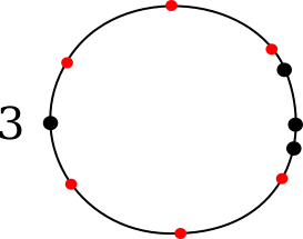
Figure 9. Weierstrass points, in red, on a genus 1 metric graph.

Example 4.4.

Suppose $\Gamma$ is a complete graph on $4$ vertices, with distinct edge lengths. This graph has genus $3$. Consider the canonical divisor $K$ on $\Gamma$, which is supported on the four trivalent vertices. The Weierstrass locus of $K$ consists of $8$ distinct points on $\Gamma$, shown in red in Figure 10.

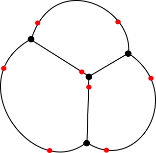
Figure 10. Metric graph with finite Weierstrass locus.

Example 4.5 (Wedge of circles).

Suppose $\Gamma$ is a wedge of $g$ circles, and let $x_{0}$ denote the point of $\Gamma$ lying on all $g$ circles. For a generic divisor class $[D_{n}]$ of degree $n$ (meaning generic inside of $\operatorname{Pic}^{n}(\Gamma)$), the $x_{0}$-reduced representative of $[D_{n}]$ consists of $n-g$ chips at $x_{0}$ and one chip in the interior of each circle. The Weierstrass locus $W(D_{n})$ contains $n-g+1$ evenly-spaced points on each circle of $\Gamma$, for a total of $g(n-g+1)$ points.

Example 4.6 (Failure of $W(D)$ to be finite).

Consider the genus $3$ graph shown in Figure 11. Suppose $D$ is a degree $4$ divisor supported on one of the bridge edges as shown. (Note that $D\sim K$.) This divisor has rank $r\leq 2$, since we cannot move the chips in $D$ to lie on three distinct loops freely. However, for any point $x$, the reduced divisor $\operatorname{red}_{x}[D]$ has at least $3$ chips at $x$.

Figure 11. Divisor on metric graph with $W(D)=\Gamma$.

Example 4.7 (Failure of $W(D)$ to be finite, v2).

Consider the genus $3$ graph shown in Figure 12. Suppose $D=K$ is the canonical divisor. By Riemann–Roch, $K$ has rank $r=2$. It is possible to move all 4 chips to lie on the middle loop, so any point in the middle loop has $\operatorname{red}_{x}[D]\geq 3x$. The Weierstrass locus $W(K)$ contains the midde loop, but not the two outer loops.

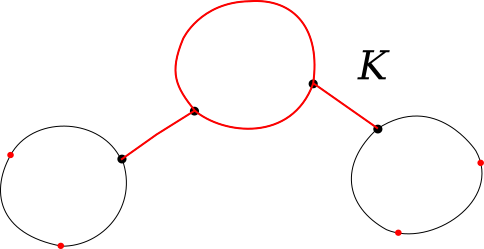
Figure 12. Metric graph with Weierstrass locus $W(K)$ not finite.

Remark 4.8.

For any metric graph with a bridge edge, it can be shown that the entire bridge edge is contained in the Weierstrass locus of the canonical divisor so in particular $W(K)$ is not finite. We omit the details.

4.3. Stable tropical Weierstrass points

In this section we define the stable Weierstrass locus $W^{\mathrm{st}}(D)$ of a divisor $D$ on a metric graph. This definition is meant to fix undesireable behavior of the naive Weierstrass locus $W(D)$. In particular, $W^{\mathrm{st}}(D)$ is always a finite set.

For the definition of break divisor, see Section 2.4.

Definition 4.9.

Let $D$ be a divisor of degree $n$ on a metric graph $\Gamma$. If $n\geq g$, the stable Weierstrass locus $W^{\mathrm{st}}(D)\subset\Gamma$ is the set of all points $x\in\Gamma$ such that

$$\operatorname{br}[D-(n-g)x]\geq x$$

where $\operatorname{br}[E]$ is the break divisor representative of the divisor class $[E]$. In other words, $x$ is a stable Weierstrass point of $D$ if

$$\text{there exists a break divisor }E\geq x\text{ such that}\qquad E+(n-g)x\in[D].$$

Note that if $D$ has degree $n=g$, then $W^{\mathrm{st}}(D)$ is exactly the support of $\operatorname{br}[D]$.

If $D$ has degree $n<g$, we define $W^{\mathrm{st}}(D)$ to be empty.

In the above definition, if $n\geq g$ then $n-g$ is the rank of a generic divisor class in $\operatorname{Pic}^{n}(\Gamma)$. If a divisor class $[D]$ in $\operatorname{Pic}^{n}(\Gamma)$ has rank $r(D)=n-g$, then $W^{\mathrm{st}}(D)\subset W(D)$; otherwise, this containment may fail to hold. In particular, we have $W^{\mathrm{st}}(D)\subset W(D)$ for all divisors of degree $n\geq 2g-1$.

Example 4.10 (Divisor with $W^{\mathrm{st}}(D)\not\subset W(D)$).

Consider the genus $3$ metric graph shown in Figure 13. The canonical divisor $K$ is indicated in black. This divisor has degree $n=4$ and rank $r(K)=2$. The divisor is special, because $r(K)>n-g=1$. On the left side, the Weierstrass locus is shown in red; the right side shows the stable Weierstrass locus. The stable Weierstrass locus consists of the midpoint of each edge. The sets $W(K)$ and $W^{\mathrm{st}}(K)$ are disjoint.

$W(K)$

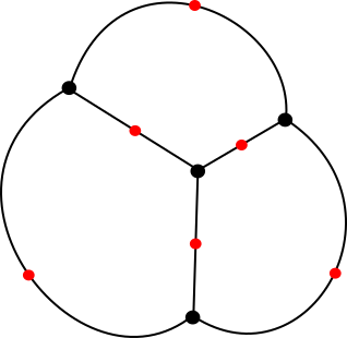
$W^{\mathrm{st}}(K)$

Figure 13. Divisor with Weierstrass locus and stable Weierstrass locus.

5. Finiteness of Weierstrass points

In this section we show that the Weierstrass locus of a generic divisor class $[D]$ on a metric graph is a finite set whose cardinality is $\#W(D)=g(n-g+1)$. We do so by studying the stable Weierstrass locus $W^{\mathrm{st}}(D)$, defined in Section 4.3.

5.1. Setup

Our main technical tool is to consider the ABKS decomposition of $\operatorname{Pic}^{g}(\Gamma)$ (see Section 2.4) and the topology of certain branched covering spaces.

As the divisor class $[D]$ varies over $\operatorname{Pic}^{n}(\Gamma)$, we realize the stable Weierstrass loci $W^{\mathrm{st}}(D)$ as the fibers of a surjective map $X\to\operatorname{Pic}^{n}(\Gamma)$. We are able to study the cardinality of $W^{\mathrm{st}}(D)$ by imposing a nice topology on $X$ and analyzing topological properties of the map $X\to\operatorname{Pic}^{n}(\Gamma)$.

Recall that $\operatorname{Br}^{g}(\Gamma)$ denotes the space of break divisors on $\Gamma$, viewed as a subspace of $\operatorname{Sym}^{g}(\Gamma)$.

Definition 5.1.

Let $\widetilde{\operatorname{Br}}^{g}(\Gamma)$ denote the space

$$\widetilde{\operatorname{Br}}^{g}(\Gamma)=\{(x,E)\in\Gamma\times\operatorname{Sym}^{g-1}(\Gamma):x+E\text{ is a break divisor}\}.$$

This defines a closed subset of the compact Hausdorff space $\Gamma\times\operatorname{Sym}^{g-1}(\Gamma)$, so $\widetilde{\operatorname{Br}}^{g}(\Gamma)$ is compact and Hausdorff.

Remark 5.2.

We may think of $\widetilde{\operatorname{Br}}^{g}(\Gamma)$ as the space of “pointed break divisors” on $\Gamma$, i.e. $\widetilde{\operatorname{Br}}^{g}(\Gamma)$ is homeomorphic to $\{(x,D)\in\Gamma\times\operatorname{Br}^{g}(\Gamma)\text{ such that }x\leq D\}$.

Let $\sigma:\widetilde{\operatorname{Br}}^{g}(\Gamma)\to\operatorname{Br}^{g}(\Gamma)$ denote the “summation” map $(x,E)\mapsto x+E$, and let $\sigma_{m}:\widetilde{\operatorname{Br}}^{g}(\Gamma)\to\operatorname{Pic}^{m+g-1}(\Gamma)$ denote the “summation with multiplicity” map defined by

$$\sigma_{m}:(x,E)\mapsto[mx+E].$$

Let $\pi_{1}:\widetilde{\operatorname{Br}}^{g}(\Gamma)\to\Gamma$ denote projection to the first factor, i.e. $\pi_{1}(x,E)=x$.

Lemma 5.3.

Suppose $[D]\in\operatorname{Pic}^{m+g-1}(\Gamma)$, and let $\sigma_{m}$ and $\pi_{1}$ be defined as above.

1. The stable Weierstrass locus $W^{\mathrm{st}}(D)$ is equal to $\pi_{1}(\sigma_{m}^{-1}[D])$.

2. The cardinality $\#W^{\mathrm{st}}(D)=\#\sigma_{m}^{-1}[D]$.

Proof.

(a) This follows from the definition of the stable Weierstrass locus.

(b) The claim is that $\pi_{1}$ is injective on the preimage $\sigma_{m}^{-1}[D]$. To see this, consider two points $(x,E)$ and $(x^{\prime},E^{\prime})\in\widetilde{\operatorname{Br}}^{g}(\Gamma)$ in the same fiber $\sigma_{m}^{-1}[D]$. This means that $[mx+E]=[mx^{\prime}+E^{\prime}]=[D]$. Suppose $\pi_{1}(x,E)=\pi_{1}(x^{\prime},E^{\prime})$, i.e. that $x=x^{\prime}$. Then

$$[D-(m-1)x]=[x+E]=[x+E^{\prime}]\in\operatorname{Pic}^{g}(\Gamma).$$

Since both $(x+E)$ and $(x+E^{\prime})$ are break divisors, the uniqueness of break divisor representatives (Theorem 2.6) implies that $E=E^{\prime}$. This shows that the restriction of $\pi_{1}$ to $\sigma_{m}^{-1}[D]$ is injective, as desired. ∎

Let $(G,\ell)$ be a combinatorial model for $\Gamma$, which induces a decomposition of break divisors $\operatorname{Br}^{g}(\Gamma)$ into a union of cells

(1) $$\operatorname{Br}^{g}(\Gamma)=\bigcup_{T\in\mathcal{T}(G)}C_{T}$$

indexed by spanning trees of $G$, where the interior of each cell $C_{T}$ is homeomorphic to an open hypercube. (See Section 2.4 or [3].) Note that $\operatorname{Br}^{g}(\Gamma)$ is homeomorphic to $\operatorname{Pic}^{g}(\Gamma)$. The ABKS decomposition (1) of $\operatorname{Br}^{g}(\Gamma)$ induces a decomposition

(2) $$\widetilde{\operatorname{Br}}^{g}(\Gamma)=\bigcup_{T\in\mathcal{T}(G)}\left(\bigcup_{e\not\in E(T)}\widetilde{C}_{T,e}\right)$$

where the second union is over edges $e$ of $G$ not contained in the spanning tree $T$. There are $g$ such edges for any $T$. Namely,

$$\widetilde{C}_{T,e}=\{(x,E)\in\widetilde{\operatorname{Br}}^{g}(\Gamma):x+E\in C_{T},\,x\in e\}$$

The map $\widetilde{\operatorname{Br}}^{g}(\Gamma)\to\operatorname{Br}^{g}(\Gamma)$ sends the cell $\widetilde{C}_{T,e}$ surjectively to $C_{T}$. On the interior $C_{T}^{\circ}$ of each cell, each fiber of $\widetilde{\operatorname{Br}}^{g}(\Gamma)\to\operatorname{Br}^{g}(\Gamma)$ contains exactly $g$ points.

If $\kappa(G)=\#\mathcal{T}(G)$ denotes the number of spanning trees of $G$, the ABKS decomposition (2) decomposes $\widetilde{\operatorname{Br}}^{g}(\Gamma)$ into a union of $g\cdot\kappa(G)$ cells.

Example 5.4.

In Figure 14, we show the decomposition of $\widetilde{\operatorname{Br}}^{2}(\Gamma)$ into six cells $\widetilde{C}_{T,e}$, where $\Gamma$ is a theta graph. This graph has genus $g=2$ and $\kappa(G)=3$ spanning trees. In this case $\operatorname{Br}^{2}(\Gamma)\cong\operatorname{Pic}^{2}(\Gamma)\cong\mathbb{R}^{2}/\mathbb{Z}^{2}$ is a genus $1$ surface (cf. Example 2.9, Theorem 2.11), and $\widetilde{\operatorname{Br}}^{2}(\Gamma)$ is a surface of genus $2$. The map $\widetilde{\operatorname{Br}}^{2}(\Gamma)\to\operatorname{Br}^{2}(\Gamma)$ is a branched double cover ramified at two points, corresponding to the two break divisors which consist of two chips at a trivalent vertex of $\Gamma$.

Figure 14. ABKS decomposition of $\widetilde{\operatorname{Br}}^{2}(\Gamma)$.

In Figure 14, each cell $\widetilde{C}_{T,e}$ shows a representative break divisor $x+E$ where the point $x\in e$ is marked with an extra outline. Edges of $\widetilde{C}_{T,e}$ which have $x$ on an endpoint of $e$ are marked in bold. Edges on the boundary are glued to the parallel boundary edge which has the same weighting (bold or unbold).

5.2. Point-set topology

Definition 5.5.

Let $M$ and $N$ be compact Hausdorff spaces, and let $N$ be path-connected. We say $p:M\to N$ is a branched covering map if

1. $p$ is continuous and surjective

2. $p$ is an open map (the image of an open set is open)

3. $p^{-1}(y)$ is finite for each $y\in N$

and there exists a closed subset $R\subset N$ such that

1. $N\backslash R$ is path-connected

2. $R$ has empty interior in $N$

3. the restriction of $p$ to $M\backslash p^{-1}(R)\to N\backslash R$ is a topological covering map.

The subspace $R$ is a ramification locus of $p$, and the preimage $p^{-1}(R)$ is a branch locus. (Note that properties (ii) and (v) imply $p^{-1}(R)$ has empty interior in $M$.)

It is straightforward to verify that the map $\widetilde{\operatorname{Br}}^{g}(\Gamma)\to\operatorname{Br}^{g}(\Gamma)$ from Section 5.1 is a branched covering. We show below, in Proposition 5.9, that in fact each $\sigma_{m}:\widetilde{\operatorname{Br}}^{g}(\Gamma)\to\operatorname{Pic}^{m+g-1}(\Gamma)$, for $m\geq 1$, is a branched covering.

Recall that a map is proper if the preimage of a compact set is compact. Recall that a map $f:X\to Y$ is a local homeomorphism if, for any $x\in X$ there is an open neighborhood $U$ containing $x$ such that $f(U)$ is open in $Y$ and the restriction $U\to f(U)$ is a homeomorphism. A covering map is always a local homemorphism, but the converse is not true.

The following lemma will be used to check the last condition (vi) in Definition 5.5, that the restriction $M\backslash p^{-1}(R)\to N\backslash R$ is a covering map.

Lemma 5.6.

Suppose $p:X\to Y$ is a local homeomorphism between locally compact, Hausdorff spaces. If $p$ is proper and surjective, then $p$ is a covering map.

This is a standard exercise in point-set topology; see e.g. [16, Lemma 2].

Lemma 5.7.

Suppose $p:M\to N$ is a branched covering with ramification locus $R\subset N$ such that the restriction $p:M\backslash p^{-1}(R)\to N\backslash R$ is a covering map of degree $d$. Then for any $y\in N$, the preimage $p^{-1}(y)$ has cardinality at most $d$.

Note: the restriction of $p$ to $M\backslash p^{-1}(R)\to N\backslash R$ has constant degree $d$ because in the definition of branched cover, $N\backslash R$ is assumed to be path connected.

Proof.

Let $y\in R$ be a point in the ramification locus, and let $x_{1},\ldots,x_{k}$ be the points in the preimage $p^{-1}(y)$. Since $M$ is Hausdorff, we may choose open neighborhoods $U_{1},\ldots,U_{k}$ with $x_{i}\in U_{i}$ which are disjoint, $U_{i}\cap U_{j}=\emptyset$. Let $C=M\backslash(U_{1}\cup\cdots\cup U_{k})$ be the complement of these neighborhoods, which is closed in $M$. Since $M$ is compact and $N$ is Hausdorff, the image $p(C)$ is closed in $N$. Thus $V=N\backslash p(C)$ is open and nonempty since $y\in V$. Note that by construction $p^{-1}(V)=M\backslash p^{-1}(p(C))\subset M\backslash C=U_{1}\cup\cdots\cup U_{k}$.

Let $U^{\prime}_{i}$ be the intersection of $p^{-1}(V)$ with $U_{i}$, which is open and nonempty because $x_{i}\in U_{i}^{\prime}$. Since the $U_{i}$ were chosen to be disjoint, $p^{-1}(V)=U_{1}^{\prime}\sqcup\cdots\sqcup U_{k}^{\prime}$.

Note that $p$ is an open map (by definition of branched cover), so the intersection $p(U_{1}^{\prime})\cap\cdots\cap p(U_{k}^{\prime})$ is an open neighborhood of $y$ in $N$. Since $R$ has empty interior in $N$, we can choose some point

$$z\in\left(p(U_{1}^{\prime})\cap\cdots\cap p(U_{k}^{\prime})\right)\backslash R\subset V\backslash R.$$

By the assumption that $M\backslash p^{-1}(R)\to N\backslash R$ is a degree $d$ covering map, the preimage $p^{-1}(z)$ contains $d$ points $w_{1},\ldots,w_{d}$. Since $z\in V$ by construction, each $w_{i}\in p^{-1}(V)=U_{1}^{\prime}\sqcup\cdots\sqcup U_{k}^{\prime}$ so $w_{i}$ lies within $U_{j}^{\prime}$ for some unique $j\in\{1,\ldots,k\}$. This relation defines a map $\pi:\{1,\ldots d\}\to\{1,\ldots,k\}$. Moreover, the map $\pi$ is surjective because $z\in p(U_{j}^{\prime})$ for each $j\in\{1,\ldots,k\}$. This proves that $k\leq d$, so the preimage $p^{-1}(y)$ has cardinality at most $d$ as desired. ∎

5.3. Proofs

Proposition 5.8.

For any divisor $D$, the stable Weierstrass locus $W^{\mathrm{st}}(D)$ is a finite subset of $\Gamma$.

Proof.

If $D$ has degree $n<g$, the stable Weierstrass locus is defined to be empty. Thus we assume below that $D$ has degree $n\geq g$.

Recall that $\widetilde{\operatorname{Br}}^{g}(\Gamma)=\{(x,E)\in\Gamma\times\operatorname{Sym}^{g-1}(\Gamma):\text{ $x+E$ is a break divisor}\}$ and that $\sigma_{m}:\widetilde{\operatorname{Br}}^{g}(\Gamma)\to\operatorname{Pic}^{m+g-1}(\Gamma)$ is defined by

$$\sigma_{m}:(x,E)\mapsto[mx+E].$$

Recall that $\pi_{1}$ denotes the projection $\pi_{1}(x,E)=x$. (See Section 5.1.) By Lemma 5.3, for a divisor $D$ of degree $m+g-1$ we have $W^{\mathrm{st}}(D)=\pi_{1}(\sigma_{m}^{-1}[D])$. Hence it suffices to show that the preimage $\sigma_{m}^{-1}[D]$ is a finite set.

Let $(G,\ell)$ be a combinatorial model for $\Gamma$, which induces the ABKS decomposition $\operatorname{Br}^{g}(\Gamma)=\bigcup_{T\in\mathcal{T}(G)}C_{T}$, where the cells $C_{T}$ are indexed by spanning trees of $G$. The ABKS decomposition of $\operatorname{Br}^{g}(\Gamma)$ induces a decomposition

$$\widetilde{\operatorname{Br}}^{g}(\Gamma)=\bigcup_{T\in\mathcal{T}(G)}\left(\bigcup_{e\not\in E(T)}\widetilde{C}_{T,e}\right).$$

Let $\sigma_{m}^{(T,e)}:\widetilde{C}_{T,e}\to\operatorname{Pic}^{m+g-1}(\Gamma)$ denote the restriction of $\sigma_{m}$ to $\widetilde{C}_{T,e}$.

Claim: The preimage of $[D]$ under $\sigma_{m}^{(T,e)}:\widetilde{C}_{T,e}\to\operatorname{Pic}^{m+g-1}(\Gamma)$ is finite.

This Claim implies that the preimage $\sigma_{m}^{-1}[D]$ is a finite set, since $\widetilde{\operatorname{Br}}^{g}(\Gamma)$ is covered by finitely many $\widetilde{C}_{T,e}$.

Proof of Claim: The map $\sigma_{m}^{T,e}:\widetilde{C}_{T,e}\to\operatorname{Pic}^{m+g-1}(\Gamma)$ is locally defined by a linear map, which we show is full rank. For a spanning tree $T=G\backslash\{e,e_{2},\ldots,e_{g}\}$, there is a natural surjective parametrization $\prod_{i=1}^{g}[0,\ell(e_{i})]\to\widetilde{C}_{T,e}$.

Let $f_{m}^{T,e}$ denote the lift of $\prod_{i=1}^{g}[0,\ell(e_{i})]\to\widetilde{C}_{T,e}\xrightarrow{}\operatorname{Pic}^{m+g-1}(\Gamma)$ to the universal cover $\mathbb{R}^{g}\to\operatorname{Pic}^{m+g-1}(\Gamma)$.

When $m=1$, coordinates may be chosen on $\mathbb{R}^{g}$ such that $f_{1}^{T,e}$ is representented by the identity matrix. Using these same coordinates on $\mathbb{R}^{g}$ (up to a translation from $\operatorname{Pic}^{g}$ to $\operatorname{Pic}^{m+g-1}$), for $m\geq 1$ the defintion $\sigma_{m}(x,E)=[mx+E]$ implies that $f^{m}_{T,e}$ is representated by the diagonal matrix

$$\begin{pmatrix}m&&\\ &1&\\ &&\ddots\\ &&&1\end{pmatrix}.$$

This shows that $f_{m}^{T,e}$ is locally injective, which implies $\sigma_{m}^{T,e}$ is locally injective as well. Thus for any $[D]\in\operatorname{Pic}^{m+g-1}(\Gamma)$, the preimage under $\sigma_{m}^{T,e}$ is a discrete subset of $\widetilde{C}_{T,e}$. Since $\widetilde{C}_{T,e}$ is compact, the preimage of $[D]$ is finite as claimed. ∎

In the following proposition, “generic” means the statement holds for $[D]\in\operatorname{Pic}^{n}(\Gamma)$ outside of a nowhere dense exceptional set.

Proposition 5.9.

For any divisor class $[D]$ of degree $n\geq g$, we have

$$\#W^{\mathrm{st}}(D)\leq g(n-g+1).$$

For a generic divisor class $[D]$ of degree $n\geq g$, the stable Weierstrass locus $W^{\mathrm{st}}(D)$ has cardinality $\#W^{\mathrm{st}}(D)=g(n-g+1)$.

Proof.

Let $\widetilde{\operatorname{Br}}^{g}(\Gamma)$, $\sigma_{m}:\widetilde{\operatorname{Br}}^{g}(\Gamma)\to\operatorname{Pic}^{m+g-1}(\Gamma)$, and $\pi_{1}:\widetilde{\operatorname{Br}}^{g}(\Gamma)\to\Gamma$ be defined as in Section 5.1. Recall that for a divisor $D$ of degree $m+g-1$, we have $\#W^{\mathrm{st}}(D)=\#(\sigma_{m}^{-1}[D])$ by Lemma 5.3. Thus it suffices to show that $\sigma_{m}:\widetilde{\operatorname{Br}}^{g}(\Gamma)\to\operatorname{Pic}^{m+g-1}(\Gamma)$ is a branched covering map of degree $gm$, for any $m\geq 1$. From this, Lemma 5.7 implies the inquality $\#W^{\mathrm{st}}(D)\leq gm$ and Definition 5.5 implies that equality holds for $[D]$ outside of the ramification locus.

(If $D$ has degree $n=m+g-1$, then $gm=g(n-g+1)$.)

Claim 1: The map $\sigma_{m}:\widetilde{\operatorname{Br}}^{g}(\Gamma)\to\operatorname{Pic}^{m+g-1}(\Gamma)$ is open, for any $m\geq 1$.

Proof of Claim 1: As above, let $(G,\ell)$ be a combinatorial model for $\Gamma$, and

$$\widetilde{\operatorname{Br}}^{g}(\Gamma)=\bigcup_{T\in\mathcal{T}(G)}\bigcup_{e\not\in E(T)}\widetilde{C}_{T,e}$$

the induced ABKS decomposition. (See Section 5.1.) The map $\sigma_{m}$ is naturally a piecewise affine map with domains of linearity $\widetilde{C}_{T,e}$.

To show that $\sigma_{m}$ is open, it suffices to check that for any $(x_{0},E_{0})\in\widetilde{\operatorname{Br}}^{g}(\Gamma)$, the image of a neighborhood contains points in all tangent directions around $\sigma_{m}(x_{0},E_{0})\in\operatorname{Pic}^{m+g-1}(\Gamma)$. To check this, we observe how $\sigma_{m}$ restricts to each domain of linearity $\widetilde{C}_{T,e}$ containing $(x_{0},E_{0})$. We will show that the behavior of $\sigma_{m}$ on tangent directions does not depend on the integer $m$.

For a point $(x_{0},E_{0})$ in $\widetilde{C}_{T,e}$, let $\operatorname{cone}(\sigma_{m}^{T,e}(x_{0},E_{0}))$ denote the positive cone in $\mathbb{R}^{g}$ spanned by

$$\sigma_{m}(x,E)-\sigma_{m}(x_{0},E_{0})\quad\text{for $(x,E)$ in a neighborhood of $(x_{0},E_{0})$ in $\widetilde{C}_{T,e}$}.$$

(Here we identify $\mathbb{R}^{g}$ with the tangent space of $\operatorname{Pic}^{0}(\Gamma)$ at the identity.) Since $\sigma_{m}$ is affine on $\widetilde{C}_{T,e}$, this cone does not depend on the neighborhood chosen. Since $m\geq 1$, the positive span of

$$\sigma_{m}(x,E)-\sigma_{m}(x_{0},E_{0})=m[x-x_{0}]+[E-E_{0}]\quad\text{for $(x,E)$ in }\widetilde{C}_{T,e}$$

is equal to the positive span of

$$\sigma_{1}(x+E)-\sigma_{1}(x_{0}+E_{0})=[x-x_{0}]+[E-E_{0}]\quad\text{for $(x,E)$ in }\widetilde{C}_{T,e},$$

so $\operatorname{cone}(\sigma_{m}^{T,e}(x_{0},E_{0}))=\operatorname{cone}(\sigma_{1}^{T,e}(x_{0},E_{0}))$. This holds for all cells $\widetilde{C}_{(T,e)}$ containing $(x_{0},E_{0})$.

Hence to show that $\sigma_{m}$ is open, it suffices to show that $\sigma_{1}:\widetilde{\operatorname{Br}}^{g}(\Gamma)\to\operatorname{Pic}^{g}(\Gamma)$ is open. This is clear from the construction of $\widetilde{\operatorname{Br}}^{g}(\Gamma)$ as a branched cover $\widetilde{\operatorname{Br}}^{g}(\Gamma)\to\operatorname{Br}^{g}(\Gamma)$, and from Theorem 2.6 which states that $\operatorname{Br}^{g}(\Gamma)\to\operatorname{Pic}^{g}(\Gamma)$ is a homeomorphism.

Claim 2: The map $\sigma_{m}:\widetilde{\operatorname{Br}}^{g}(\Gamma)\to\operatorname{Pic}^{m+g-1}(\Gamma)$ is a branched cover, for any $m\geq 1$.

Proof of Claim 2: In the definition of branched cover, Definition 5.5, condition (ii) was verfied by Claim 1 and condition (iii) was verified by Proposition 5.8. Condition (i) is clear.

We first identify a ramification locus $R$ for $\sigma_{m}$, and then apply Lemma 5.6 to show that the restriction of $\sigma_{m}$ away from $R$ is a covering map.

Let $\operatorname{Br}^{g}(\Gamma)=\bigcup_{T\in\mathcal{T}(G)}C_{T}$ be the ABKS decomposition induced by a combinatorial model $\Gamma=(G,\ell)$ (see Section 2.4). Let $Z^{(2)}\subset\operatorname{Br}^{g}(\Gamma)$ denote the union of faces of $C_{T}$ of codimension at least $2$, and let $U^{(2)}=\operatorname{Br}^{g}(\Gamma)\backslash Z^{(2)}$. In other words,

$$U^{(2)}=\bigcup_{T\in\mathcal{T}(G)}\{\text{interior $C_{T}^{\circ}$ of $C_{T}$}\}\cup\{\text{interiors of facets of $\partial C_{T}$}\}.$$

More concretely in terms of break divisors, given a set of edges $e_{1},\ldots,e_{g}$ in $G$ whose complement is a spanning tree, $U^{(2)}$ contains break divisors which are a sum of $g$ points taken from the interior of each $e_{1},e_{2},\ldots,e_{g}$, and divisors which are a sum of one endpoint of $e_{1}$ and a point in the interior of each $e_{2},\ldots,e_{g}$. We assume our combinatorial model $(G,\ell)$ is chosen to have no loops, so that each cell $C_{T}$ in the ABKS decomposition has $2g$ distinct boundary facets.

Note that for a break divisor $E$,

(3) $$\text{if }E\in U^{(2)},\text{ the support of $E$ consists of $g$ distinct points}.$$

We let $\widetilde{Z}^{(2)}$ and $\widetilde{U}^{(2)}$ denote the preimages of $Z^{(2)}$ and $U^{(2)}$ under $\sigma:\widetilde{\operatorname{Br}}^{g}(\Gamma)\to\operatorname{Br}^{g}(\Gamma)$. Note that with respect to the ABKS decomposition

$$\widetilde{\operatorname{Br}}^{g}(\Gamma)=\bigcup_{T\in\mathcal{T}(G)}\bigcup_{e\not\in E(T)}\widetilde{C}_{T,e},$$

$\widetilde{Z}^{(2)}$ is the union of codimension $2$ faces of $\widetilde{C}_{T,e}$, and $\widetilde{U}^{(2)}=\widetilde{\operatorname{Br}}^{g}(\Gamma)\backslash\widetilde{Z}^{(2)}$. Thus $\widetilde{Z}^{(2)}$ is a closed subset of codimension $2$ and $\widetilde{U}^{(2)}$ is a dense open subset of $\widetilde{\operatorname{Br}}^{g}(\Gamma)$.

Next, let $R=R_{m}=\sigma_{m}(\widetilde{Z}^{(2)})$. We will show that $R$ is a valid ramification locus for the branched cover $\sigma_{m}$. The conditions (iv) and (v) hold because $R$ is a codimesion $2$ submanifold of the connected manifold $\operatorname{Pic}^{m+g-1}(\Gamma)$. It remains to check condition (vi), that the restriction

(4) $$\sigma_{m}|_{\widetilde{\operatorname{Br}}^{g}(\Gamma)\backslash\sigma_{m}^{-1}(R)}:\widetilde{\operatorname{Br}}^{g}(\Gamma)\backslash\sigma_{m}^{-1}(R)\to\operatorname{Pic}^{m+g-1}(\Gamma)\backslash R$$

away from ramification is a covering map. To check this condition, we apply Lemma 5.6. It is clear that the domain and codomain of (4) are locally compact Hausdorff spaces. The map in (4) is surjective by construction; it is proper because $\sigma_{m}$ is a map from a compact space to a Hausdorff space, hence proper. It remains to check that (4) is a local homeomorphism, which we leave for the next claim. Note that the domain of (4) is contained in $\widetilde{U}^{(2)}$:

$$\widetilde{\operatorname{Br}}^{g}(\Gamma)\backslash\sigma_{m}^{-1}(R)=\widetilde{\operatorname{Br}}^{g}(\Gamma)\backslash\sigma_{m}^{-1}(\sigma_{m}(\widetilde{Z}^{(2)}))\subset\widetilde{\operatorname{Br}}^{g}(\Gamma)\backslash Z^{(2)}=\widetilde{U}^{(2)}.$$

Assuming Claim 3, Lemma 5.6 implies that $\sigma_{m}$ is a covering map away from the ramification locus $R$, which completes the proof of Claim 2.

Claim 3: The restriction of $\sigma_{m}$ to $\widetilde{U}^{(2)}\to\operatorname{Pic}^{m+g-1}(\Gamma)$ is a local homeomorphism, for any $m\geq 1$.

Proof of Claim 3: First consider $m=1$. Observation (3) implies that

(5) the restriction $$\sigma_{1}|_{\widetilde{U}^{(2)}}:\widetilde{U}^{(2)}\to U^{(2)} g$$ is a (unbranched) covering of degree .

Since $U^{(2)}\subset\operatorname{Pic}^{g}(\Gamma)$ is open, it follows that $\sigma_{1}:\widetilde{U}^{(2)}\to\operatorname{Pic}^{g}(\Gamma)$ is a local homeomorphism.

Recall that $\widetilde{U}^{(2)}$ is the union of the interior of $\widetilde{C}_{T,e}$ and the interiors of facets of $\partial\widetilde{C}_{T,e}$, over all $(T,e)$. In the interior of $\widetilde{C}_{T,e}$, $\sigma_{m}$ can be expressed as a full-rank linear map so it is a local homeomorphism. Now consider how $\sigma_{m}$ acts near the interior of a facet of $\partial\widetilde{C}_{T,e}$. We claim that each facet is shared by exactly two cells.

Suppose $T=G\backslash\{e=e_{1},e_{2},\ldots,e_{g}\}$. There are $2g$ facets of the boundary $\partial\widetilde{C}_{T,e}$, indexed by choosing an edge $e_{j}$ and choosing one of its two endpoints. For a fixed index $j$ in $\{1,\ldots,g\}$ and $v(e_{j})$ a fixed endpoint of $e_{j}$, the corresponding facet of $\partial\widetilde{C}_{T,e}$ consists of pairs $(x,E)\in\widetilde{\operatorname{Br}}^{g}(\Gamma)$ of the form

(6) $$\widetilde{F}_{(T,e)}^{(j,v)}=\{(x=x_{1},E=x_{2}+\cdots+x_{g}):\begin{array}[]{l}x_{j}=v(e_{j}),\\ x_{i}\in e_{i}^{\circ}\text{ for }i=1,\ldots g,\,i\neq j\}\end{array}$$

Let $G_{j}=T\cup e_{j}$. Since $e_{j}\not\in T$, the graph $G_{j}$ contains a unique cycle, which must contain $v(e_{j})\in e_{j}$. Let $e_{j}^{\prime}$ be the unique edge $\neq e_{j}$ in this cycle which also borders $v(e_{j})$, and let $T^{\prime}=G_{j}\backslash e_{j}^{\prime}=(T\cup e_{j})\backslash e_{j}^{\prime}$. Then $\widetilde{C}_{T^{\prime},e^{\prime}}$ is the only other cell containing the facet (6), where $e^{\prime}=e_{1}^{\prime}$ if $j=1$, and $e^{\prime}=e$ otherwise. The facet (6) is then the relative interior of $\widetilde{C}_{T,e}\cap\widetilde{C}_{T^{\prime},e^{\prime}}$

As before, let $f_{m}^{T,e}$ denote the lift of $\widetilde{C}_{T,e}\to\operatorname{Pic}^{m+g-1}(\Gamma)$ in the diagram

and define $f_{m}^{T^{\prime},e^{\prime}}$ analogously.

We may choose coordinates (depending on $T$) on $\mathbb{R}^{g}$ such that

$$\text{the matrix representing $f_{m}^{T,e}$ is}\quad\begin{pmatrix}m&&\\ &1&\\ &&\ddots\\ &&&1\end{pmatrix}.$$

In these same coordinates, the matrix representing $f_{m}^{T^{\prime},e^{\prime}}$ is

$$\begin{pmatrix}-m&&\\ *&1&\\ *&&\ddots\\ *&&&1\end{pmatrix}\text{ if }j=1,\quad\text{ or }\quad\begin{pmatrix}m&&*&\\ &\ddots&*&\\ &&-1&\\ &&*&\ddots\end{pmatrix}\text{ if }j\in\{2,\ldots,g\}.$$

(Recall that $j$ is the index specifying which edge $e_{j}\in G\backslash T$ has a break divisor chip on one of its endpoints; $e_{j}$ is the unique edge in $T^{\prime}\backslash T$.) This shows that $\sigma_{m}$ is a local homeomorphism in a neighborhood of the chosen facet of $\partial\widetilde{C}_{T,e}$.

Claim 4: The branched cover $\sigma_{m}:\widetilde{\operatorname{Br}}^{g}(\Gamma)\to\operatorname{Pic}^{m+g-1}(\Gamma)$ has degree $gm$.

Proof of Claim 4: When $m=1$, it is clear that $\sigma_{1}:\widetilde{\operatorname{Br}}^{g}(\Gamma)\to\operatorname{Pic}^{g}(\Gamma)\cong\operatorname{Br}^{g}(\Gamma)$ is a degree $g$ branched cover. When $m>1$, we note that $\sigma_{m}$ differs from $\sigma_{1}$ by a scaling factor of $m$, i.e. on a sufficiently small neighborhood $U\subset\widetilde{\operatorname{Br}}(\Gamma)$, the Haar measure of $\sigma_{m}(U)$ is $m$-times as large as the Haar measure of $\sigma_{1}(U)$. (The space $\operatorname{Pic}^{m+g-1}(\Gamma)$ carries a Haar measure since it is a torsor for the compact topological group $\operatorname{Pic}^{0}(\Gamma)$.) This implies that the degree of $\sigma_{m}$ as a branched cover must be $m$ times the degree of $\sigma_{1}$, so $\sigma_{m}$ must have degree $gm$ as desired. ∎

Theorem A.

Let $\Gamma$ be a compact, connected metric graph of genus $g$.

1. For a generic divisor class of degree $n\geq g$, the Weierstrass locus $W(D)$ is finite with cardinality $\#W(D)=g(n-g+1)$. For a generic divisor class of degree $n<g$, $W(D)$ is empty.

2. For an arbitrary divisor class of degree $n\geq g$, the stable Weierstrass locus $W^{\mathrm{st}}(D)$ is finite with cardinality

   $$\#W^{\mathrm{st}}(D)\leq g(n-g+1),$$

   and equality holds for a generic divisor class.

Proof.

Part (b) is a restatement of Proposition 5.9.

For part (a), first suppose $n<g$. The space $\operatorname{Pic}^{n}(\Gamma)$ has dimension $g$, while the subspace of effective divisor classes has dimension at most $n$. Thus a generic divisor class in $\operatorname{Pic}^{n}(\Gamma)$ is not effective, assuming $n<g$. By Remark 4.2, the Weierstrass locus is empty for a non-effective divisor class.

Now suppose $n\geq g$. To prove (a), it suffices to show that $W(D)=W^{\mathrm{st}}(D)$ for a generic divisor class, since then part (b) applies. To compare $W(D)$ with $W^{\mathrm{st}}(D)$, we construct a map $X\to\operatorname{Pic}^{n}(\Gamma)$ whose fiber over $[D]$ is the Weierstrass locus $W(D)$; this parallels our construction in Section 5.1 for $W^{\mathrm{st}}(D)$.

For $m\geq 1$, let $s_{m}:\Gamma\times\operatorname{Sym}^{g-1}(\Gamma)\to\operatorname{Pic}^{m+g-1}(\Gamma)$ denote the map

$$s_{m}(x,E)=[mx+E].$$

Let $\pi_{1}:\Gamma\times\operatorname{Sym}^{g-1}(\Gamma)\to\Gamma$ denote projection to the first factor.

The Riemann–Roch formula, Theorem 2.13, implies that a generic divisor class $[D]\in\operatorname{Pic}^{m+g-1}(\Gamma)$ has rank $r(D)=(m+g-1)-g=m-1$. For such a divisor,

$$W(D)=\{x\in\Gamma:[D-mx]\geq 0\}=\pi_{1}(s_{m}^{-1}[D]).$$

Recall that $W^{\mathrm{st}}(D)=\pi_{1}(\sigma_{m}^{-1}[D])$, where $\sigma_{m}$ is defined to be the restriction of $s_{m}$ to the subset $\widetilde{\operatorname{Br}}^{g}(\Gamma)\subset\Gamma\times\operatorname{Sym}^{g-1}(\Gamma)$; note that

(7) $$\sigma_{m}^{-1}[D]=s_{m}^{-1}[D]\cap\widetilde{\operatorname{Br}}^{g}(\Gamma)\subset s_{m}^{-1}[D].$$

Under the genericity assumption on $[D]$, we have

$$W^{\mathrm{st}}(D)=\pi_{1}(\sigma_{m}^{-1}[D])\subset\pi_{1}(s_{m}^{-1}[D])=W(D).$$

Using part (b), this observation implies that a generic Weierstrass locus $W(D)$ contains at least $g(n-g+1)$ points.

We consider when $W(D)$ can be strictly larger than $W^{\mathrm{st}}(D)$. By (7), this happens only if $s_{m}^{-1}[D]$ is not contained in $\widetilde{\operatorname{Br}}(\Gamma)$; equivalently, only if $[D]$ lies in the image of $(\Gamma\times\operatorname{Sym}^{g-1}(\Gamma))\backslash\widetilde{\operatorname{Br}}(\Gamma)$ under $s_{m}$.

Claim: The image $s_{m}(\,(\Gamma\times\operatorname{Sym}^{g-1}(\Gamma))\backslash\widetilde{\operatorname{Br}}(\Gamma)\,)$ has dimension $g-1$ in $\operatorname{Pic}^{m+g-1}(\Gamma)$.

It is clear that $s_{m}$ is piecewise affine on $\Gamma\times\operatorname{Sym}^{g-1}(\Gamma)$, with domains of linearity indexed by $g$-tuples of edges $(e_{1};e_{2},\ldots,e_{g})$, up to reordering the edges $e_{2},\ldots,e_{g}$. (Here we choose an arbitrary combinatorial model $(G,\ell)$ for $\Gamma$.) The edges $e_{i}$ are not necessarily distinct.

If the edges $(e_{1};e_{2},\ldots,e_{g})$ form the complement of a spanning tree $T$ in $G$, then the corresponding domain is in $\widetilde{\operatorname{Br}}^{g}(\Gamma)$; namely, it is the cell $\widetilde{C}_{T,e_{1}}$ in the notation of Section 5.1. Conversely, if the edges $(e_{1};e_{2},\ldots,e_{g})$ are not the complement of a spanning tree in $G$, then either some edge is repeated or the edges contain a cut set of $G$. In either case, the fibers of $s_{m}:\Gamma\times\operatorname{Sym}^{g-1}(\Gamma)\to\operatorname{Pic}^{m+g-1}(\Gamma)$ have dimension at least $1$ over the interior of the corresponding domain (see [15, Proposition 13]), so the image of this domain under $s_{m}$ has dimension at most $g-1$. This proves the claim.

The claim implies that for a generic divisor class $[D]$, the preimage $s_{m}^{-1}[D]$ is contained in $\widetilde{\operatorname{Br}}^{g}(\Gamma)$. By (7) this implies $W(D)=W^{\mathrm{st}}(D)$, as desired. ∎

6. Distribution of Weierstrass points

In this section we prove Theorem B. We show that for a degree-increasing sequence of generic divisors on a metric graph, the Weierstrass points become distributed with respect to the Zhang canonical measure (defined in Section 3.3). We also give a quantitative version of this distribution result, Theorem C.

Our proofs of Theorems B and C work unchanged when $W(D)$ is replaced by the stable Weierstrass locus $W^{\mathrm{st}}(D)$.

6.1. Examples

First we consider some low genus examples of Weierstrass points converging to a limiting distribution.

Example 6.1 (Genus $0$ metric graph).

Let $\Gamma$ be a genus $0$ metric graph. For any divisor $D_{n}$, the associated Weierstrass locus $W(D_{n})$ is empty so $\delta_{n}=0$. All edges are bridges, so the canonical measure is $\mu=0$.

Example 6.2 (Genus $1$ metric graph).

Let $\Gamma$ be a genus $1$ metric graph which consists of a loop of length $L$. For a divisor $D_{n}$ of degree $n$, the Weierstrass locus $W_{n}=W(D_{n})$ consists of $n$ evenly-spaced points (“torsion points”) around the loop. The distance between adjacent points is ${L}/{n}$, so on a segment $e$ of length $\ell({e})$ the number of Weierstrass points is bounded by

$$\frac{\ell({e})}{L/n}-1\leq\#(W_{n}\cap e)\leq\frac{\ell({e})}{L/n}+1.$$

This means the associated discrete measure $\delta_{n}=\frac{1}{n}\sum_{x\in W_{n}}\delta_{x}$ satisfies

$$\delta_{n}(e)=\frac{\#(W_{n}\cap e)}{n}\qquad\Rightarrow\qquad\frac{\ell({e})}{L}-\frac{1}{n}\leq\delta_{n}(e)\leq\frac{\ell({e})}{L}+\frac{1}{n}.$$

Hence $\delta_{n}(e)\to\frac{\ell({e})}{L}=\mu(e)$ as $n\to\infty$.

6.2. Proofs

We now address the limiting distribution of Weierstrass points $W(D_{n})$ as $n\to\infty$ in the case of an arbitrary metric graph $\Gamma$.

Lemma 6.3.

Suppose the Weierstrass locus $W(D)$ is finite. Let $r=r(D)$.

1. If $x$ is in the interior of a segment, $\operatorname{red}_{x}[D]$ contains at most $r+1$ chips at $x$.

2. If $x$ is in the interior of a segment $e\subset\Gamma$, $\operatorname{red}_{x}[D]$ contains at most $r+1$ chips on $e$ (including its endpoints).

Proof.

(a) Suppose $\operatorname{red}_{x}[D]$ contains $r+2$ chips at $x$. Then for sufficiently small $\epsilon$ we can move $r+1$ of these chips together for a distance $\epsilon$ in one direction, while moving $1$ chip a distance $(r+1)\epsilon$ in the other. This gives a positive-length interval in $W(D)$, a contradiction.

(b) Suppose $\operatorname{red}_{x}[D]$ contains $r+2$ chips on the closed segment $e$. Note that at least $r$ of these chips must be at $x$, in the interior of $e$. By chip-firing, we may move all $r+2$ chips to a single point $x^{\prime}$ in the interior of $e$. Then part (a) applies. ∎

Theorem B.

Let $\{D_{n}:n\geq 1\}$ be a sequence of divisors on $\Gamma$ with $\deg D_{n}=n$. Let $W_{n}$ be the Weierstrass locus of $D_{n}$. Suppose each $W_{n}$ is a finite set, and let

$$\delta_{n}=\frac{1}{n}\sum_{x\in W_{n}}\delta_{x}$$

denote the normalized discrete measure on $\Gamma$ associated to $W_{n}$. Then as $n\to\infty$, the measures $\delta_{n}$ converge weakly to the Zhang canonical measure $\mu$ on $\Gamma$.

Recall that by definition of weak convergence, Theorem B says that for any continuous function $f:\Gamma\to\mathbb{R}$, as $n\to\infty$ we have convergence

$$\frac{1}{n}\sum_{x\in W_{n}}f(x)=:\int_{\Gamma}f(x)\delta_{n}(dx)\quad\to\quad\int_{\Gamma}f(x)\mu(dx).$$

Proof of Theorem B.

To show weak convergence of measures on $\Gamma$ it suffices to show convergence when integrated against step functions. Hence it suffices to integrate the measures against the indicator function of an arbitrary segment of $\Gamma$.

Let $e$ be a segment in the metric graph $\Gamma$ of length $\ell({e})$, with endpoints $s$ and $t$. Let $W_{n}\cap e$ denote the set of Weierstrass points of $D_{n}$ lying on the segment $e$. It suffices to show that

(8) $$\lim_{n\to\infty}\frac{\#(W_{n}\cap e)}{n}=\mu(e).$$

Recall that by Proposition 3.24,

$$\mu(e)=\frac{\ell({e})}{\ell({e})+\ell_{\text{eff}}({\Gamma\backslash e})}$$

where $\ell_{\text{eff}}({\Gamma\backslash e})$ denotes the effective resistance between the endpoints of $e$ when the interior of $e$ is removed from $\Gamma$. (If $\Gamma\backslash e$ is disconnected, $\ell_{\text{eff}}({\Gamma\backslash e})=+\infty$ and $\mu(e)=0$.) We prove (8) by relating each side to the slope of a piecewise linear function on $\Gamma$.

For the right-hand side of (8), consider the voltage function $j_{t}^{s}:\Gamma\to\mathbb{R}$ (see Section 3.1). The voltage drop in $\Gamma$ between endpoints of $e$ is the effective resistance

$$j_{t}^{s}(s)-j_{t}^{s}(t)=r(s,t)=\frac{\ell({e})\ell_{\text{eff}}({\Gamma\backslash e})}{\ell({e})+\ell_{\text{eff}}({\Gamma\backslash e})},$$

by the parallel rule for effective resistance. Thus we have

(9) $$\frac{j_{t}^{s}(s)-j_{t}^{s}(t)}{\ell({e})} =\frac{\ell_{\text{eff}}({\Gamma\backslash e})}{\ell({e})+\ell_{\text{eff}}({\Gamma\backslash e})}=1-\frac{\ell({e})}{\ell({e})+\ell_{\text{eff}}({\Gamma\backslash e})}=1-\mu(e).$$

(Recall that this slope can be interpreted as the current flowing along the segment $e$ from $s$ to $t$, since $\text{current}=\frac{\text{voltage drop}}{\text{resistance}}$.)

To connect $j_{t}^{s}$ to the left-hand side of (8), we consider a sequence of piecewise-linear functions which are “discrete approximations” of $j_{t}^{s}$, and show that certain slopes in these functions are related to the number of Weierstrass points.

Let $f_{n}$ be the piecewise $\mathbb{Z}$-linear function on $\Gamma$ satisfying

$$\operatorname{\Delta}(f_{n})=\operatorname{red}_{t}[D_{n}]-\operatorname{red}_{s}[D_{n}]\qquad\text{and}\qquad f_{n}(t)=0.$$

(Recall that $\operatorname{red}_{x}[D]$ denotes the $x$-reduced divisor linearly equivalent to $D$.) By Proposition 3.7, as $n\to\infty$ we have uniform convergence

(10) $$\frac{1}{n}f_{n}\to j_{t}^{s}.$$

Thus to show (8) using (9) and (10), it suffices to show that

(11) $$\lim_{n\to\infty}\frac{1}{n}\left(\frac{f_{n}(s)-f_{n}(t)}{\ell({e})}\right)=1-\lim_{n\to\infty}\frac{\#(W_{n}\cap e)}{n}.$$

We first give an intuitive explanation for (11): the slope of the function $f_{n}$ on a directed segment is equal to the net flow of chips across the segment, as we move from $\operatorname{red}_{s}[D_{n}]$ to $\operatorname{red}_{t}[D_{n}]$ along any path in the linear system $|D_{n}|$. If we follow $\operatorname{red}_{x}[D_{n}]$ as $x$ varies from $s$ to $t$, we have $n-g$ chips moving in the “forward” direction of $e$ (following $x$) and some number of chips moving in the reverse direction one-by-one. The number of “reverse-moving” chips is equal to $\#(W_{n}\cap e)$, since $x$ is in $W_{n}$ exactly when $\operatorname{red}_{x}[D_{n}]$ has an “extra” chip at $x$, i.e. when the $n-g$ chips on $x$ collide with a reverse-moving chip. Thus the net number of chips moving across the segment $e$ is equal to $(n-g)-\#(W_{n}\cap e)$, up to some bounded error due to boundary behavior. This yields (11) after dividing by $n$ and taking $n\to\infty$.

Now we give a rigorous argument. Let $w_{1},w_{2},\ldots,w_{m}$ denote the Weierstrass points on $e$, ordered from $s$ to $t$, so that $m=\#(W_{n}\cap e)$. Here we use the hypothesis that $W_{n}$ is finite. (Note that $m=m_{n}$ depends on $n$.)

We partition the segment $e=[s,t]$ into subintervals $[s,w_{1}],[w_{1},w_{2}],\ldots,[w_{m},t]$. (It is possible that the intervals $[s,w_{1}]$ and $[w_{m},t]$ are degenerate.) Let $\ell({[w_{i},w_{i+1}]})$ denote the length of the segment $[w_{i},w_{i+1}]\subset e$. We have

$$\ell({e})=\ell({[s,w_{1}]})+\ell({[w_{1},w_{2}]})+\cdots+\ell({[w_{m-1},w_{m}]})+\ell({[w_{m},t]}).$$

For each $i=1,2,\ldots,m-1$, let $g_{n}^{(i)}$ denote the function in $\operatorname{PL}_{\mathbb{Z}}(\Gamma)$ satisfying

$$\operatorname{\Delta}(g_{n}^{(i)})=\operatorname{red}_{w_{i+1}}[D_{n}]-\operatorname{red}_{w_{i}}[D_{n}],$$

and let $g_{n}^{(0)}$ and $g_{n}^{(m)}$ denote functions satisfying

$$\operatorname{\Delta}(g_{n}^{(0)})=\operatorname{red}_{w_{1}}[D_{n}]-\operatorname{red}_{s}[D_{n}],\qquad\text{and}\qquad\operatorname{\Delta}(g_{n}^{(m)})=\operatorname{red}_{t}[D_{n}]-\operatorname{red}_{w_{m}}[D_{n}].$$

By adding an appropriate constant, we may assume that $g_{n}^{(i)}(t)=0$ for each $i=0,1,\ldots,m$. By telescoping of poles and zeros, we have

$$\operatorname{\Delta}(f_{n})=\operatorname{\Delta}(g_{n}^{(0)})+\operatorname{\Delta}(g_{n}^{(1)})+\cdots+\operatorname{\Delta}(g_{n}^{(m)}).$$

With the additional constraint that $f_{n}(t)=\sum_{i}g_{n}^{(i)}(t)=0$, this implies that

(12) $$f_{n}=g_{n}^{(0)}+g_{n}^{(1)}+\cdots+g_{n}^{(m)}.$$

Thus we can compute $f_{n}(s)-f_{n}(t)$ by summing $\sum_{i=0}^{m}\left(g^{(i)}(s)-g^{(i)}(t)\right)$.

To analyze the slopes of $g^{(i)}$ on segment $e$, we make use of Lemma 6.3. This information is sufficient to deduce all slopes over $e$. We may assume without loss of generality that $r(D_{n})=n-g$, since this holds for $n\geq 2g-1$.

For $i=1,2,\ldots,m-1$, the function $g_{n}^{(i)}$ has slope $-(n-g)$ on the interval $[w_{i},w_{i+1}]$, and slope $1$ on $e$ outside of this interval. See Figure 15.

Figure 15. Function $g_{n}^{(i)}$ having zeros $\operatorname{red}_{w_{i+1}}[D_{n}]$ and poles $\operatorname{red}_{w_{i}}[D_{n}]$, with slopes are indicated above each affine part.

Thus we have

$$g_{n}^{(i)}(s)-g_{n}^{(i)}(t) =(n-g)\ell({[w_{i},w_{i+1}]})-\ell({[s,w_{i}]})-\ell({[w_{i+1},t]})$$

(13) $$=(n-g+1)\ell({[w_{i},w_{i+1}]})-\ell({e}).$$

For $i=0$ and $i=m$, to write an expression for $g_{n}^{(i)}(x)-g_{n}^{(i)}(t)$ we need to set additional notation. If $\operatorname{red}_{s}[D_{n}]$ has a chip in the interior of $e$, let $y$ be the position of this chip (which is unique by Lemma 6.3); otherwise, let $y=t$. Similarly, let $z$ be the position of the unique chip of $\operatorname{red}_{t}[D_{n}]$ in the interior of $e$ if it exists; otherwise let $z=s$. We have

$$g_{n}^{(0)}(s)-g_{n}^{(0)}(t) =(n-g)\ell({[s,w_{1}]})-\ell({[w_{1},y]})$$

(14) $$=(n-g+1)\ell({[s,w_{1}]})-\ell({[s,y]})$$

and

$$g_{n}^{(m)}(s)-g_{n}^{(m)}(t) =(n-g)\ell({[w_{m},t]})-\ell({[z,w_{m}]})$$

(6.2’) $$=(n-g+1)\ell({[w_{m},t]})-\ell({[z,t]})$$

Figure 16. Function $g_{n}^{(0)}$ having zeros $\operatorname{red}_{w_{1}}[D_{n}]$ and poles $\operatorname{red}_{s}[D_{n}]$.

Thus adding the expressions (6.2) and (6.2) together, by (12) we have

$$f_{n}(s)-f_{n}(t) =(n-g+1)\big{(}\ell({[s,w_{1}]})+\ell({[w_{1},w_{2}]})+\cdots+\ell({[w_{m-1},w_{m}]})+\ell({[w_{m},t]})\big{)}$$

$$\qquad-\ell({[s,y]})-(m-1)\ell({e})-\ell({[z,t]})$$

$$=(n-g+1)\ell({e})-(m-1)\ell({e})-\ell({[s,y]})-\ell({[z,t]})$$

$$=(n-g-m+2)\ell({e})-\ell({[s,y]})-\ell({[z,t]})$$

$$=(n-g-m)\ell({e})+(\ell({e})-\ell({[s,y]}))+(\ell({e})-\ell({[z,t]}))$$

$$=(n-g-m)\ell({e})+\ell({[y,t]})+\ell({[s,z]}).$$

Since $0\leq\ell({[y,t]})+\ell({[s,z]})\leq 2\ell({e})$ and $m=\#(W_{n}\cap e)$, this shows that

$$n-g-\#(W_{n}\cap e)\leq\frac{f_{n}(s)-f_{n}(t)}{\ell({e})}\leq n-g+2-\#(W_{n}\cap e).$$

Dividing by $n$ and taking the limit $n\to\infty$ yields (11) as desired. ∎

Theorem 6.4.

Consider the setup of Theorem B.

1. Suppose each $[D_{n}]$ is generic in $\operatorname{Pic}^{n}(\Gamma)$. Then each $W_{n}$ is finite and we have weak convergence $\delta_{n}\to\mu$.

2. Let $W^{\mathrm{st}}_{n}=W^{\mathrm{st}}(D_{n})$ be the stable Weierstrass locus, and define $\delta^{\text{st}}_{n}$ analogously to $\delta_{n}$. For any divisors $\{D_{n}:n\geq 1\}$ we have weak convergence $\delta^{\text{st}}_{n}\to\mu$.

Proof.

(a) This is part of Theorem A.

(b) We may follow the same argument used in Theorem B, except in place of $\operatorname{red}_{x}[D_{n}]$ we consider the “stable reduced divisor”

$$\operatorname{red}^{\mathrm{st}}_{x}[D_{n}]:=(n-g)x+\operatorname{br}[D_{n}-(n-g)x].$$

With this change in the definitions of $f_{n}$ and $g_{n}^{(i)}$, equations (6.2) and (6.2) still hold, as does the convergence (10). ∎

Theorem C (Quantitative distribution of $W(D)$).

Let $\Gamma$ be a metric graph of genus $g$, let $D_{n}$ be a divisor class of degree $n>g$ and let $W_{n}$ denote the Weierstrass locus of $D_{n}$. Suppose $W_{n}$ is finite. Let $\mu$ denote the Zhang canonical measure on $\Gamma$.

1. For any segment $e$ in $\Gamma$,

   $$n\mu(e)-2g\leq\#(W_{n}\cap e)\leq n\mu(e)+g+2.$$

2. If $e$ is a segment of $\Gamma$ with $\mu(e)>\frac{2g}{n}$, then $e$ contains at least one Weierstrass point of $D_{n}$.

3. For a fixed continuous function $f:\Gamma\to\mathbb{R}$,

   $$\frac{1}{n}\sum_{x\in W_{n}}f(x)=\int_{\Gamma}f(x)\mu(dx)+O\left(\frac{1}{n}\right).$$

Proof.

It is clear that part (b) follows from part (a), since $\#(W_{n}\cap e)$ must be an integer. Part (c) is a straightforward extension of (a).

We now prove part (a). Let $f_{n}$ be the piecewise linear function satisfying $\operatorname{\Delta}(f_{n})=\operatorname{red}_{t}[D_{n}]-\operatorname{red}_{s}[D_{n}]$ and $f_{n}(t)=0$, where $s$ and $t$ are the endpoints of $e$. By Proposition 3.8, we have

$$|(f_{n}-(n-g)j_{t}^{s})^{\prime}(x)|\leq g$$

so

$$|f_{n}^{\prime}(x)|\leq(n-g)|j^{\prime}(x)|+g.$$

Recall that for $x$ on the segment $e$, $|j^{\prime}(x)|=1-\mu(e)$. Thus we have the bound

$$|f_{n}^{\prime}(x)|\leq n-n\mu(e)+\mu(e)g.$$

Moreover the proof of Theorem B shows that

$$n-g-\#(W_{n}\cap e)\leq|f_{n}^{\prime}(x)|.$$

Combining these inequalities gives

$$n\mu(e)-(1+\mu(e))g\leq\#(W_{n}\cap e).$$

Finally, the inequality $\mu(e)\leq 1$ from Corollary 3.25 yields the lower bound in (a).

We similarly obtain the upper bound

$$\#(W_{n}\cap e)\leq n\mu(e)+g+2$$

by combining the inequalities

$$n-n\mu(e)-(2-\mu(e))g\leq|f_{n}^{\prime}(x)|\quad\text{and}\quad|f_{n}^{\prime}(x)|\leq n-g-\#(W_{n}\cap e)+2$$

and $\mu(e)\geq 0$ from Corollary 3.25. ∎

7. Appendix: Theta intersections

In this appendix we give an alternate description of the Weierstrass locus $W(D)$ as the intersection of two polyhedral subcomplexes of complementary dimension in $\operatorname{Pic}^{g-1}(\Gamma)$. This allows us to give an alternate proof that $W(D)$ is finite for a generic divisor class $[D]$. In this perspective, the stable Weierstrass locus $W^{\mathrm{st}}(D)$ naturally appears as the stable tropical intersection of these two subsets.

Throughout this section (including the above paragraph), we assume that the divisor class $[D]$ is (Riemann–Roch) nonspecial, meaning that its rank satisfies

$$r(D)=\begin{cases}\deg(D)-g&\text{if }\deg(D)\geq g,\\ -1&\text{otherwise}.\end{cases}$$

A generic divisor class in $\operatorname{Pic}^{n}(\Gamma)$ is nonspecial. If $n\geq 2g-1$, all divisors in $\operatorname{Pic}^{n}(\Gamma)$ are nonspecial.

7.1. Intersection with $\Theta$

Recall that the theta divisor $\Theta\subset\operatorname{Pic}^{g-1}(\Gamma)$ is the space of degree $g-1$ divisor classes which have an effective representative;

$$\Theta=\{[D]\in\operatorname{Pic}^{g-1}(\Gamma):[D]\geq 0\}.$$

Given a divisor $D$ of degree $n\geq g$, let $\Phi_{D}:\Gamma\to\operatorname{Pic}^{g-1}(\Gamma)$ denote the map

$$\Phi_{D}:x\mapsto[D-(n-g+1)x].$$

If $D$ has degree $n<g$ let $\Phi_{D}:x\mapsto[D]$ be the constant map. Note that the map $\Phi_{D}$ depends only on the divisor class $[D]$. If $D$ is nonspecial, the Weierstrass locus of $D$ is equal to the intersection $\Phi_{D}(\Gamma)\cap\Theta$, pulled back to $\Gamma$ from $\operatorname{Pic}^{g-1}(\Gamma)$.

Proposition 7.1.

Let $D$ be a divisor of degree $n\geq g$, and let $\Phi_{D}:\Gamma\to\operatorname{Pic}^{g-1}(\Gamma)$ be the map $\Phi_{D}(x)=[D-(n-g+1)x]$. If $D$ is a nonspecial,

$$W(D)=\Phi_{D}^{-1}(\Phi_{D}(\Gamma)\cap\Theta).$$

Proof.

This follows from the definition of Weierstrass locus, if $D$ has rank $n-g$. ∎

Proposition 7.2.

Suppose $\Gamma$ is a bridgeless metric graph. If $D$ has degree $n\geq g$, the map $\Phi_{D}:\Gamma\to\operatorname{Pic}^{g-1}(\Gamma)$ is locally injective (i.e. an immersion).

Proof.

The map $\Phi_{D}$ may be expressed as a composition of three maps

$$\Phi_{D}:\Gamma\xrightarrow{\alpha}\operatorname{Pic}^{1}(\Gamma)\xrightarrow{\beta}\operatorname{Pic}^{n-g+1}(\Gamma)\xrightarrow{\gamma}\operatorname{Pic}^{g-1}(\Gamma),$$

where $\alpha$ sends $x\mapsto[x]$, $\beta$ sends $[E]\mapsto[(n-g+1)E]$, and $\gamma$ sends $[E]\mapsto[D-E]$. The map $\gamma=\gamma_{D}$ is a homeomorphism. The map $\beta$ is a $(n-g+1)^{g}$-fold covering map, so it is a local homeomorphism if $n\geq g$. Thus it suffices to verify that the first map $\alpha$ is locally injective.

This follows from the Abel–Jacobi theorem for metric graphs, see e.g. Baker–Faber [7, Theorem 4.1 (3)(4)]. Note that $\operatorname{Pic}^{1}(\Gamma)$ is (non-canonically) isomorphic to the Jacobian $\operatorname{Jac}(\Gamma)=\operatorname{Pic}^{0}(\Gamma)$ by choosing a basepoint $x_{0}$ to subtract. ∎

If $\Gamma$ contains bridge segments, let $\Gamma_{\text{/(br)}}$ denote the metric graph obtained from $\Gamma$ by contracting all bridges. Let $S_{\text{(br)}}\subset\Gamma_{\text{/(br)}}$ denote the set of points which were bridges in $\Gamma$.

Lemma 7.3.

Let $\pi:\Gamma\to\Gamma_{\text{/(br)}}$ denote the canonical map contracting all bridge segments of $\Gamma$, which induces $\pi_{*}:\operatorname{Pic}^{n}(\Gamma)\to\operatorname{Pic}^{n}(\Gamma_{\text{/(br)}})$ for all $n$. For any divisor $D$ on $\Gamma$,

$$W(D)=\pi^{-1}W(\pi_{*}(D)).$$

Proof.

On $\Gamma$ the linear equivalence map $x\mapsto[x]$ factors through $\pi:\Gamma\to\Gamma_{\text{/(br)}}$; i.e. we have a commuting diagram

Using this, the result is clear from the definition of $W(D)$. ∎

Lemma 7.4.

Suppose $S\subset\Gamma$ is a finite set of points in a metric graph $\Gamma$. For a generic divisor class $[D]$, the intersection $W(D)\cap S$ is empty.

Proof.

It suffices to consider when $S=\{s\}$ contains one point. Assuming $D$ is nonspecial, which holds for generic $[D]\in\operatorname{Pic}^{n}(\Gamma)$, we have $s\in W(D)$ if and only if

$$[D-(n-g+1)s]\text{ is effective}\quad\Leftrightarrow\quad[D]=[(n-g+1)s+E]\text{ for some }[E]\in\Theta.$$

Since $\Theta$ has dimension $g-1$, the space $\{[D]=[(n-g+1)s+E]:[E]\in\Theta\}$ also has dimension $g-1$. Hence a generic class $[D]$ has $s\not\in W(D)$. ∎

Theorem 7.5.

For a generic divisor class $[D]$ in $\operatorname{Pic}^{n}(\Gamma)$, the Weierstrass locus $W(D)$ is finite.

Proof.

If $n<g$, then a generic divisor class in $\operatorname{Pic}^{n}(\Gamma)$ is not effective because the image of $\operatorname{Sym}^{n}(\Gamma)\to\operatorname{Pic}^{n}(\Gamma)$ has dimension at most $n$, while $\operatorname{Pic}^{n}(\Gamma)$ has dimension $g$. For a non-effective divisor class $[D]$, the Weierstrass locus $W(D)$ is empty.

Now suppose $n\geq g$. By Riemann–Roch, a generic divisor class in $\operatorname{Pic}^{n}(\Gamma)$ has rank $r(D)=n-g$. (By the above paragraph, $r(K-D)=-1$ generically.) Thus, it suffices to show that $W(D)$ is finite for a generic nonspecial divisor class.

Case 1: $\Gamma$ is bridgeless. As above, let $\Phi_{D}:\Gamma\to\operatorname{Pic}^{g-1}(\Gamma)$ be the map $\Phi_{D}(x)=[D-(n-g+1)x]$. Recall that the Weierstrass locus $W(D)$ is equal to

$$W(D)=\Phi_{D}^{-1}(\Phi_{D}(\Gamma)\cap\Theta)\subset\Gamma$$

where $\Theta=\{[E]\in\operatorname{Pic}^{g-1}(\Gamma):[E]\geq 0\}$ is the theta divisor. Note that as $[D]$ varies, the image $\Phi_{D}(\Gamma)$ varies by translation inside $\operatorname{Pic}^{g-1}(\Gamma)$.

Recall that $\Theta$ is a $(g-1)$-dimensional polyhedral complex with finitely many facets, and $\Phi_{D}(\Gamma)$ is a 1-dimensional polyhedral complex with finitely many segments. This implies that the space of translations which cause $\Phi_{D}(\Gamma)$ to intersect $\Theta$ non-transversally has dimension at most $g-1$. Hence for a generic divisor class $[D]$, the intersection $\Phi_{D}(\Gamma)\cap\Theta$ is transverse.

Suppose all intersections in $\Phi_{D}(\Gamma)\cap\Theta$ are transverse, and occur in the interiors of the respective segment and facet. Recall that $\Phi_{D}$ is locally injective by Proposition 7.2. If $\Phi_{D}$ sends $x\in\Gamma$ to a transverse intersection, then $x$ must have some neighborhood $U\subset\Gamma$ such that $\Phi_{D}(U\backslash\{x\})$ is disjoint from $\Theta$. This means that $W(D)=\Phi_{D}^{-1}(\Phi_{D}(\Gamma)\cap\Theta)$ is a discrete subset of $\Gamma$. Because $\Gamma$ is compact, this implies $W(D)$ is finite.

Case 2: $\Gamma$ has bridge segments. Let $\pi:\Gamma\to\Gamma_{\text{/(br)}}$ denote the map contracting all bridge segments of $\Gamma$. Let $S_{\text{(br)}}\subset\Gamma_{\text{/(br)}}$ denote the image of all bridges, which is a finite subset of $\Gamma_{\text{/(br)}}$. Note that $\pi$ restricts to an injection away from $\pi^{-1}S_{\text{(br)}}$.

By Lemma 7.4, a generic divisor class $[D]\in\operatorname{Pic}^{n}(\Gamma_{\text{/(br)}})$ has $W(D)$ disjoint from $S_{\text{(br)}}$. Since $\pi$ induces a homeomorphism $\pi_{*}:\operatorname{Pic}^{n}(\Gamma)\to\operatorname{Pic}^{n}(\Gamma_{\text{/(br)}})$, this implies that a generic class $[D]\in\operatorname{Pic}^{n}(\Gamma)$ has $W(\pi_{*}[D])$ disjoint from $S_{\text{(br)}}$. The result then follows from Lemma 7.3 and Case 1. ∎

7.2. Stable Weierstrass locus

In this section we describe the relation of the current setup, involving the theta divisor $\Theta$, and the stable Weierstrass locus defined in Section 4.3.

Proposition 7.6.

Suppose $\Gamma$ is a bridgeless metric graph of genus $g$. Let $D$ be a divisor of degree $g$, and let $\Phi_{D}:\Gamma\to\operatorname{Pic}^{g-1}(\Gamma)$ send $\Phi_{D}(x)=[D-x]$. Then the break divisor $\operatorname{br}[D]$ is equal to

$$\operatorname{br}[D]=\Phi_{D}^{-1}(\Phi_{D}(\Gamma)\cap^{\mathrm{st}}\Theta)$$

where $\Theta$ is the theta divisor and $\cap^{\mathrm{st}}$ denotes stable tropical intersection.

Proof.

Let us denote $\operatorname{br}^{*}[D]:=\Phi_{D}^{-1}(\Phi_{D}(\Gamma)\cap^{\mathrm{st}}\Theta)$. For a generic divisor class $[D]\in\operatorname{Pic}^{g}(\Gamma)$, the intersection $\Phi_{D}(\Gamma)\cap\Theta$ is transverse so

$$\operatorname{br}^{*}[D]=\{x\in\Gamma:[D-x]\geq 0\},$$

i.e. $\operatorname{br}^{*}[D]$ contains the support of any effective representative of $[D]$. Generically, the class $[D]$ contains a single effective representative so $\operatorname{br}^{*}:\operatorname{Pic}^{g}(\Gamma)\to\operatorname{Sym}^{g}(\Gamma)$ defines a generic section of the linear equivalence map $\operatorname{Sym}^{g}(\Gamma)\to\operatorname{Pic}^{g}(\Gamma)$.

By general properties of stable tropical intersection, the map $\operatorname{br}^{*}:\operatorname{Pic}^{g}(\Gamma)\to\operatorname{Sym}^{g}(\Gamma)$ is continuous. But by Theorem 2.6, the break divisor map $\operatorname{br}$ is the unique continuous section of $\operatorname{Sym}^{g}(\Gamma)\to\operatorname{Pic}^{g}(\Gamma)$ so we must have $\operatorname{br}^{*}[D]=\operatorname{br}[D]$. ∎

8. Appendix: Tropicalizing Weierstrass points

In this section, we describe how the Weierstrass locus for a tropical curve can be related to the Weierstrass locus for an algebraic curve. The key result is Baker’s Specialization Lemma [5, Lemma 2.8]; here we use a more general version given by Jensen–Payne [17] in the language of Berkovich analytic spaces. The results of this section are not needed for any later sections of the paper.

Throughout this section, let $K$ denote an algebraically closed field equipped with a nontrivial non-Archimedean valuation $v:K^{\times}\to\mathbb{R}$; we assume $K$ is complete with respect to $v$.

Theorem 8.1 (Specialization Lemma [17, Lemma 2.4]).

Suppose $X$ is a smooth projective algebraic curve over $K$. Let $\Gamma$ be a skeleton on the Berkovich analytification $X^{an}$, let $\rho:X^{an}\to\Gamma$ be the retration to the skeleton and let $\rho_{*}:\operatorname{Div}(X)\to\operatorname{Div}(\Gamma)$ denote the induced map on divisors. Then for any divisor $D\in\operatorname{Div}(X)$,

$$r_{X}(D)\leq r_{\Gamma}(\rho_{*}(D)).$$

Here $r_{X}$ denotes the dimension of a complete linear system $|D|$ on $X$, and $r_{\Gamma}$ denotes the Baker–Norine rank on $\Gamma$ (see Section 2.6).

Theorem 8.2.

Consider the setup of Theorem 8.1. For any divisor $D\in\operatorname{Div}(X)$ such that $\rho_{*}(D)\in\operatorname{Div}(\Gamma)$ is Riemann–Roch nonspecial, we have

$$\rho_{*}(W_{X}(D))\subseteq W_{\Gamma}(\rho_{*}(D)).$$

Proof.

The map $\rho_{*}$ respects degree; let $n=\deg(D)=\deg(\rho_{*}(D))$. Recall that $\rho_{*}(D)$ is nonspecial means that

$$r_{\Gamma}(\rho_{*}(D))=\max\{n-g,\,-1\}.$$

In this case, Theorem 8.1 implies $r_{X}(D)\leq\max\{n-g,\,-1\}$ while Riemann–Roch implies $r_{X}(D)\geq\max\{n-g,\,-1\}$ for any divisor. Thus $r_{X}(D)=r_{\Gamma}(\rho_{*}(D))$.

Let $r$ denote the rank in either sense. If $x\in W_{X}(D)$, we have

$$r_{X}(D-(r+1)x)\geq 0.$$

By Theorem 8.1 and linearity of $\rho_{*}$, this implies

$$r_{\Gamma}(\rho_{*}(D-(r+1)x))=r_{\Gamma}(\rho_{*}(D)-(r+1)\rho_{*}(x))\geq 0.$$

This means $\rho_{*}(x)\in W_{\Gamma}(\rho_{*}(D))$ as claimed. ∎

The conclusion of Theorem 8.2 also holds for $D=K_{X}$ the canonical divisor, and $\rho_{*}(K_{X})\sim K_{\Gamma}$. This was observed by Baker in [5, Corollary 4.9].

References

- [1] O. Amini, Reduced divisors and embeddings of tropical curves, Trans. Amer. Math. Soc. 365 (2013), 4851–4880.
- [2] O. Amini, Equidistribution of Weierstrass points on curves over non-Archimedean fields, preprint, arXiv:1412.0926v1, 2014.
- [3] Y. An, M. Baker, G. Kuperberg and F. Shokrieh, Canonical representatives for divisor classes on tropical curves and the matrix tree theorem, Forum Math. Sigma 2 (2014), e25.
- [4] S. J. Arakelov, Intersection theory of divisors on an arithmetic surface, Izv. Akad. Nauk 8 (1974), 1167–1180.
- [5] M. Baker, Specialization of linear systems from curves to graphs, Algebra Number Theory 2 no. 6 (2008), 613–653.
- [6] M. Baker and X. Faber, Metrized graphs, Laplacian operators, and electrical networks, in Quantum graphs and their applications, volume 415 of Contemp. Math., pages 15–33. Amer. Math. Soc., Providence, RI, 2006.
- [7] M. Baker and X. Faber, Metric properties of the tropical Abel-Jacobi map, J. Algebr. Comb. 33 (2011), 349–381.
- [8] M. Baker and S. Norine, Riemann-Roch and Abel-Jacobi theory on a finite graph, Adv. in Math. 215 (2007), 766–788.
- [9] M. Baker and R. Rumely, Harmonic analysis on metrized graphs, Canad. J. Math. 59 (2007), no. 2, 225–275.
- [10] M. Baker and F. Shokrieh, Chip-firing games, potential theory on graphs, and spanning trees, J. Combin. Theory Ser. A 120 (2013), no. 1, 164–182. arXiv:1107.1313v2, 2012.
- [11] T. Chinburg and R. Rumely, The capacity pairing, J. Reine Angew. Math. 434 (1993), 1–44.
- [12] R. M. Foster, The average impedance of an electrical network, in Reissner Anniversary Volume, Contributions to Applied Mechanics, 333–340, J. W. Edwards, Ann Arbor, MI, 1949.
- [13] A. Gathmann and M. Kerber, A Riemann-Roch theorem in tropical geometry, Math. Z. 259 (2008), no. 1, 217–230.
- [14] A. Gross, F. Shokrieh and L. Tóthmérész, Effective divisor classes on metric graphs, preprint, arXiv:1807.00843v1 (2018).
- [15] C. Haase, G. Musiker and J. Yu, Linear systems on tropical curves, Math. Z. 270 (2012), no. 3-4, 1111–1140.
- [16] C. Ho, A note on proper maps, Proc. Amer. Math. Soc. 51 (1975), no. 1, 237–241.
- [17] D. Jensen and S. Payne, Tropical independence I: Shapes of divisors and a proof of the Gieseker–Petri theorem, Algebra Number Theory 8 (2014) no. 9, 2043–2066.
- [18] Y. Luo, Tropical convexity and canonical projections, preprint, arXiv:1304.7963 (2013).
- [19] G. Mikhalkin and I. Zharkov, Tropical curves, their Jacobians and theta functions, preprint, arXiv:0612267v2 (2007).
- [20] R. Miranda, Algebraic Curves and Riemann Surfaces, Graduate Studies in Mathematics vol. 5, American Mathematical Society, Providence, RI, 1995.
- [21] D. B. Mumford, Curves and their Jacobians, The University of Michigan Press, Ann Arbor, MI, 1977.
- [22] A. Neeman, The distribution of Weierstrass points on a compact Riemann surface, Ann. of Math. (2) 120 (1984), no. 2, 317–328.
- [23] B. A. Olsen, On higher order Weierstrass points, Ann. of Math. (2) 95 (1972), no. 2, 357–364.
- [24] S. Zhang, Admissible pairing on a curve, Invent. Math. 112 (1993), no. 1, 171–193.