Thermomagnetic stability in isotropic type-II superconductors under multicomponent magnetic fields

Abstract

The goal of this research is the study of the thermomagnetic consequences in isotropic type-II superconductors, subjected to multi-component magnetic fields $\mathbf{H}_{a}=H_{ay}\hat{y}+H_{az}\hat{z}$, because the instability field $\mathbf{H}_{fi}$ is closely related with a flux jump occurrence. At the critical-state model framework, once the Lorentz $\mathbf{F}_{L}$ and pinning forces $\mathbf{F}_{P}$ are at equilibrium, the current density reaches a critical value $j_{c}$ and a stationary magnetic induction distribution $\mathbf{B}$ is established. The equilibrium of forces is analytically solved considering that the pinning force is mainly affected by temperature increments; the energy dissipation is incorporated throughout the heat equation at the adiabatic regime. The theory is able to obtain the instability field according to the thermal bath and applied field values; moreover, it provides of instability field branches comprising both partial and full penetrates states. With this information is possible to construct a field-temperature map. The results are compared with already published experimental data, finding a qualitatively agreement between them. This theoretical study works with a first order perturbation, then the perturbation presents a periodical behavior along the thickness direction; considering this environment it is constructed the magnetic induction distributions which resemble flexible cantilever structures.

I Introduction

Since a half century to find criteria to realize and control how type-II superconductors remain in a stable state, with the maximum trapped flux and the minimum of losses, has been a research subject. For each value of the magnetic induction in the range $B_{c1}<B<B_{c2}$ there is a specific maximum value of the current density $j_{c}$ which if it is exceeded causes that the superconductor enters into a resistive state up to change its phase and enters into the normal state. The current density $j_{c}(B,T)$ is called the critical value for specific values of the induction B and temperature T.

At present, it is clear the Lorentz force $F_{L}$ nature as well as it drives the vortices to move across the sample, however, the pinning force $F_{P}$ origin is so complex that an exhaustive description requires another studies, out of those presented here; for the time being it is enough to model $F_{P}$ as an average of an uniform distribution of pinning sites, qualitatively described by the Kim-Anderson model for $j_{c}(B,T)$ PhysRev.129.528 ; PhysRevB.42.10773 .

There are a list of facts related with the type-II superconductors behavior: at the equilibrium of forces, the magnetic induction is smooth and the slope at each point of the sample corresponds to a critical current density $j_{c}$, which generally speaking depends on the magnetic induction and has a curvature; on increasing the current density above a certain maximum value the Lorentz force becomes greater than the pinning force, so the vortex starts to move; this leads to the continuous evolution of Joule’s heat, the temperature may rise above $T_{c}$, and the superconductor will enter into the normal state; the material stability depends on the ramp rate of the applied magnetic field, the temperature, the specif heat of the material, the heat release conditions of the experimental set up, the geometry as well as the preparation sample. Because such variables are correlated it is desirable to know its participation on such process al2013stabilization .

In the present article, the balance of forces scheme is used to describe the problem of instabilities sosnowski1983flux ; sosnowski:jpa-00245326 ; sosnowski1986influence ; PhysRev.161.404 ; wipf1991review . It is knows that the thermomagnetic stability description requires to take into account the equilibrium between the Lorentz, pinning and viscous forces. The external field drives the vortices throughout the Lorentz force $\mathbf{F}_{L}=\mathbf{j}\times\mathbf{B}=(1/\mu_{0})\nabla\times\mathbf{B}\times\mathbf{B}$ and their movement can be prevented by pinning $\mathbf{F}_{P}$ or viscous $\mathbf{F}_{\mathit{v}}$ forces, therefore the critical state corresponds to the equilibrium forces $\mathbf{F}_{L}+\mathbf{F}_{P}+\mathbf{F}_{v}=\mathbf{0}$. The viscous force is a dynamical force which depends on the vortex velocity, in our theory we assume that the vortex velocity is such that the viscous force is not comparable with the pinning force therefore its contribution is neglected.

Therefore, we study an isotropic superconductor embedded in a thermal bath with temperature $T_{B}$ and subject to an external magnetic field $H_{a}$, for each external magnetic field change, the flux front goes deep forward inside up to a $x_{0}$ point. As $H_{a}$ changes as $H_{a}+\Delta H_{a}$ the temperature changes as $T_{B}+\Delta T$ due to Joule’s heat, since the magnetic diffusion time is much smaller than the thermal diffusion time, the magnetic induction reaches an stationary state before the temperature be homogenized at the thermal bath. A consequence of this fact is that it decreases the critical current density, promoting that the flux front goes deeper across the sample.

The equilibrium force condition provides of isothermic profiles of magnetic induction $B_{i}(x)$, in our study we are going to consider that an increment $\Delta H_{a}$ will produce a new magnetic profile, given by $\mathbf{B}=\mathbf{B}_{i}+\Delta\mathbf{B}$. At this new configuration, the Lorentz and pinning forces are written as $\mathbf{F}_{L}(\mathbf{B}_{i}+\Delta\mathbf{B})=\mathbf{F}_{L}(\mathbf{B}_{i})+\Delta\mathbf{F}_{L}(\mathbf{B}_{i},\Delta\mathbf{B})$ and $\mathbf{F}_{P}(\mathbf{B}_{i}+\Delta\mathbf{B})=\mathbf{F}_{P}(\mathbf{B}_{i})+\Delta\mathbf{F}_{P}(\mathbf{B}_{i},\Delta\mathbf{B})$, where the condition $\Delta\mathbf{F}_{L}+\Delta\mathbf{F}_{P}=\mathbf{0}$ is fulfilled.

The changes on the external field produce thermal variations which can produce instabilities on the system, however, the magnetic properties of the superconducting material will stay stable under such changes meanwhile the pinning force subjects the Lorentz force, under these conditions the net transport of vortices is null. The stability condition can be written as follows:

$$|\mathbf{F}_{L}(\mathbf{B}_{i})+\Delta\mathbf{F}_{L}(\mathbf{B}_{i},\Delta\mathbf{B})|\underset{\mathrm{Instability}}{\overset{\mathrm{Stability}}{\lessgtr}}|\mathbf{F}_{P}(\mathbf{B}_{i})+\Delta\mathbf{F}_{P}(\mathbf{B}_{i},\Delta\mathbf{B})|$$ (1)

The aim of this article is to find the instability magnetic field $H_{fi}$, which delimits the magnetic stability of the superconductor, defined by the condition (1). It is considered a semi-infinite-isotropic type-II superconductor plate, with thickness $d$ along the $x-\mathrm{direction}$ and its surface lying on the $yz-\mathrm{plane}$, under the effect of an applied magnetic field $\mathbf{H}_{a}=H_{ay}\hat{y}+H_{az}\hat{z}$. At this situation, the so-called parallel geometry, all the electromagnetic vectors are coplanar to the $yz$ surface and functions only of the variable $x$. It is assumed that the applied field is larger than the first critical field $H_{c1}$, thus the approximation $\mu_{0}\mathbf{H}a=\mathbf{B}(x=0)=\mathbf{B}(x=d)$ is fullfiled.

This manuscript is divided as follows: In section (II) one can find an analytic expression for the isothermal magnetic induction $\mathbf{B}_{i}$ obtained from the balance of forces; in order to simplify the notation, it is removed the subindex $``i"$ since the main purpose of this paper is the resulting field $\mathbf{B}_{i}+\Delta\mathbf{B}$. In section (III) throughout the deviation forces balance, after a small increment of the applied magnetic field occurs, is obtained expressions for $\Delta B$ and $\mu_{0}H_{fi}$ at the adiabatic regime. Finally, in section (IV) it is presented an example where it is compared the theory proposed and experimental data, obtaining an $H-T$ instability diagram, $B$ and temperature profiles.

II Equilibrium between Lorentz and pinning forces and the isothermal approach

This teoretical development starts considering the equilibrium between Lorentz and pinning forces $\mathbf{F}_{L}=-\mathbf{F}_{P}$; the external field drives the vortices motion through the Lorentz force $\mathbf{F}_{L}=\mathbf{j}\times\mathbf{B}=(1/\mu_{0})\nabla\times\mathbf{B}\times\mathbf{B}$, however, such movement can be prevented by pinning centers represented with an average force knows as the pinning force $\mathbf{F}_{P}$. In the following lines, is it shown explicit expressions for both forces in terms of the magnetic induction. From the balance of forces it will obtain the equation which governs the magnetic induction. Let us show this fact.

Writing the magnetic induction as $\mathbf{B}=B(x)\hat{e}$, with $\hat{e}=\cos\phi\hat{x}+\sin\phi\hat{y}$, since the system is at the parallel geometry, the Ampere’s law looks like:

$$\mu_{0}\mathbf{j}=B\left(-\frac{d\phi}{dx}\right)\hat{e}-\frac{dB}{dx}(\hat{e}\times\hat{x})$$ (2)

The Lorentz force is

$$\mu_{0}\mathbf{F}_{L}=-B^{2}\frac{d\phi}{dx}\hat{e}\times\hat{e}-B\frac{dB}{dx}(\hat{e}\times\hat{x}\times\hat{e})=-B\frac{dB}{dx}\hat{x},$$ (3)

while the pinning force is modelled as

$$\mu_{0}\mathbf{F}_{P}=\mu_{0}jB\cos\theta\hat{x};$$ (4)

here $\theta$ is the angle of $\mathbf{j}$ respect to $\mathbf{B}$. Notice the change of sign of the equation (4) according to

$$\cos\theta=\left\{\begin{array}[]{lr}<0,&0\leq x<d/2\\ >0,&d/2<x\leq d\end{array}\right.,$$ (7)

therefore when the sample is at critical state $j=j_{c}$ and $\theta=0,\pi$ at $0\leq x<d/2$, $d/2<x\leq d$, respectively. It is defined the function $f_{H}=2H_{e}(x-d/2)-1$, where $H_{e}(x-d/2)$ is the Heaviside function, to rewrite the equation (4) as $\mu_{0}\mathbf{F}_{P}=\mu_{0}j_{c}Bf_{H}\hat{x}$. It is employed the well-known phenomenological relation for the critical current density $j_{c}(B,T)$:

$$j_{c}(B,T)=\alpha(T)\frac{j_{0}}{\left(1+\frac{B}{B^{*}}\right)^{n}}$$ (8)

where $\alpha$ is a function of the temperature; $n$ and $B^{*}$ are parameters. Now, defining $b=1+B/B^{*}$, the pinning and Lorentz forces acquire the form

$$\mu_{0}\mathbf{F}_{P}=\alpha(T)\mu_{0}j_{0}B^{*}\frac{(b-1)}{b^{n}}f_{H}\hat{x},\quad\mu_{0}\mathbf{F}_{L}=-(b-1)\frac{db}{dx}(B^{*})^{2}\hat{x},$$ (9)

with the forces balance, it is found the equation that governs the magnetic induction behavior

$$\frac{db}{dx}=\frac{\alpha(T)\mu_{0}j_{0}}{B^{*}}\frac{f_{H}}{b^{n}}.$$ (10)

For the research purposes of this work, in the following lines, isothermic magnetic induction profiles will be obtained; in this case $\alpha$ is constant.

The ordinary differential equation (10) is solved considering the boundary conditions $B(x=0)=B(x=d)=\mu_{0}H_{a}$. The analytic solution is:

$$b^{n+1}=f_{H}\frac{\alpha\mu_{0}j_{0}(n+1)}{B^{*}}(x-x_{H})+b_{a}^{n+1},$$ (11)

here $b_{a}=1+\mu_{0}H_{a}/B^{*}$ and $x_{H}=d/2\,H_{e}(x-d/2)$. The field $b^{n+1}$ describes a master curve, which is a simple straight line ROMERO-SALAZAR2013 . The sample symmetry makes that the flux front ($x_{f}$ for $x\in[0,d/2)$ and $x^{\prime}_{f}=d-x_{0}$ for $x\in(d/2,d]$) goes forward up to reach the middle as the applied field be equal to the penetration field; the flux front for field values larger than the penetration field is given by the constant value$x_{f}=x^{\prime}_{f}=d/2$. One should notice that the solution (11), valid for $x\in[0,d]$, includes non physical solutions for partial penetrate states if $b^{n+1}<0$ . To avoid this issue, one should work with heuristic solutions, valid for both states, as the following

$$b^{n+1}=\left\{\begin{array}[]{lr}1&x_{f}<x<d-x_{f};\\ b_{a}^{n+1}-\displaystyle\frac{\alpha\mu_{0}j_{0}(n+1)}{B^{*}}x&0\leq x\leq x_{f};\\ b_{a}^{n+1}+\displaystyle\frac{\alpha\mu_{0}j_{0}(n+1)}{B^{*}}(x-\frac{d}{2})&d-x_{f}<x\leq d.\end{array}\right.$$ (15)

The magnetic induction components will not be necessary for the purposes of this work, however, they can be written as follows

$$b_{y}=b\cos\phi+(1-\cos\phi),\quad b_{z}=b\sin\phi+(1-\sin\phi)$$

where $\phi=-\tan^{-1}(H_{az}/H_{ay})$.

To finish this section, it is calculated the flux front and the penetration field.The first one $x_{f}=x_{f}(\mu_{0}H_{a})$ can be obtained for both partial and full penetrate states. For partial penetrate states one has that $B(x=x_{f})=0$ or $b(x=x_{f})=1$, therefore, using the equation (15) is obtained that,

$$x_{f}=(1-b_{a}^{n+1})\frac{B^{*}}{\alpha\mu_{0}j_{0}(n+1)}.$$ (16)

For full penetrate states the flux front is always at $x_{f}=d/2$, then the field minimum $b_{h}=b(x_{f}=d/2)$ is

$$b^{n+1}_{h}=b_{a}^{n+1}-\frac{\alpha\mu_{0}j_{0}(n+1)}{B^{*}}\frac{d}{2},$$ (17)

where $b_{h}=1+B_{h}/B^{*}$ with $B_{h}=B(x=d/2)$. The first penetration field corresponds to $b_{h}=1$,

$$b_{p}^{n+1}=\alpha(n+1)\frac{B_{0}}{B^{*}}+1,$$ (18)

where $B_{0}=\mu_{0}j_{0}d/2$ is the Bean first penetration field.

III Fluctuations balance and the instability field $H_{fi}$

III.1 Fluctuations balance

When a magnetic field $\mu_{0}\mathbf{H}_{a}$ is applied on a superconducting material, the Lorentz and pinning forces vary up to reach the equilibrium $\mathbf{F}_{L}+\mathbf{F}_{P}=0$. If $\mu_{0}\mathbf{H}_{a}$ is increased $\mu_{0}\Delta\mathbf{H}_{a}$, the superconductor suffers a change of state related with Lorentz and pinning forces changes $\Delta\mathbf{F}_{L}=\mathbf{F}^{{}^{\prime}}_{L}-\mathbf{F}_{L}$ and $\Delta\mathbf{F}_{P}=\mathbf{F}^{{}^{\prime}}_{P}-\mathbf{F}_{P}$, here $\mathbf{F}^{\prime}_{L}$ and $\mathbf{F}^{\prime}_{P}$ denote the Lorentz and pinning forces due to $\mu_{0}\mathbf{H}_{a}+\mu_{0}\Delta\mathbf{H}_{a}$. At the equilibrium of forces $\mathbf{F}^{{}^{\prime}}_{L}+\mathbf{F}^{{}^{\prime}}_{P}=0$ or $\Delta\mathbf{F}_{L}+\Delta\mathbf{F}_{P}=0$. The magnetic induction $\mathbf{B}$ corresponds to $\mu_{0}\mathbf{H}_{a}$ while $\mathbf{B}+\Delta\mathbf{B}$ it is the outcome of a perturbation $\mu_{0}\Delta\mathbf{H}_{a}$ added to $\mu_{0}\Delta\mathbf{H}_{a}$. Here $\Delta\mathbf{B}$ corresponds to the magnetic induction deviation due to the perturbated material state, both have the same direction $\mathbf{B}=B\hat{e}$ and $\Delta\mathbf{B}=\Delta B\hat{e}$, consequently $\mathbf{B}+\Delta\mathbf{B}=(B+\Delta B)\hat{e}$.

Let us show expressions for both Lorentz and pinning forces changes. The Lorentz force change is obtained from $\mu_{0}\Delta\mathbf{F}_{L}=\mu_{0}\mathbf{F}_{L}(\mathbf{B}+\Delta\mathbf{B})-\mu_{0}\mathbf{F}_{L}(\mathbf{B})=\mu_{0}\Delta F_{L}\hat{x}$, its unique component is

$$\mu_{0}\Delta F_{L}=-B\frac{d\Delta B}{dx}-\Delta B\frac{dB}{dx},$$ (19)

the quadratic term $\Delta B(d(\Delta B)/dx)$ will be neglected. Using the variable $b=1+B/B^{*}$ and $db/dx=\alpha\mu_{0}j_{0}f_{H}/B^{*}(1/b^{n})$, the former equation is rewritten as

$$\mu_{0}\Delta F_{L}=-\left\{(b-1)\frac{d\Delta B}{db}+\Delta B\right\}\frac{\alpha(T)\mu_{0}j_{0}f_{H}}{b^{n}}.$$ (20)

It is assumed that the pinning force is a functional $F_{P}=F_{P}(T,B;x)$, then it has the total derivative of $F_{P}$ is $dF_{p}/dx=\partial_{x}F_{P}+\partial_{T}F_{P}dT/dx+\partial_{B}F_{P}dB/dx$. Integrating it is obtained

$$\mu_{0}\Delta F_{p}=\mu_{0}\!\!\!\!\!\!\!\!\int\limits_{F_{P}}^{F_{P}+\Delta F_{P}}\!\!\!\!\!\!\!\!F^{\prime}_{P}dF^{\prime}_{P}\;\;=\mu_{0}\!\!\!\!\!\int\limits_{T}^{T+\Delta T}\!\!\!\!\!\!\partial_{T^{\prime}}F_{P}dT^{\prime}\;\;+\mu_{0}\!\!\!\!\!\int\limits_{B}^{B+\Delta B}\!\!\!\!\!\!\partial_{B^{\prime}}F_{P}dB^{\prime},$$

where $\partial_{x}F_{P}=0$ because it does not depend explicitly on the position. It is assumed that $\partial_{T}F_{P}$ and $\partial_{B}F_{P}$ stay approximately constants during the integration. With these arguments an approximate expression of the pinning force change is obtained:

$$\mu_{0}\Delta F_{P} \approx \partial_{T}(\mu_{0}F_{P})\Delta T+\partial_{b}(\mu_{0}F_{P})\frac{\Delta B}{B^{*}}$$ (21)

$$= \mu_{0}j_{0}B^{*}f_{H}\partial_{T}\alpha\frac{b-1}{b^{n}}\Delta T+\frac{\mu_{0}\alpha j_{0}B^{*}f_{H}}{b^{n+1}}\left\{(-n)(b-1)+b\right\}\frac{\Delta B}{B^{*}}$$

The equilibrium between forces demands that $\mu_{0}\Delta\mathbf{F}_{L}=-\mu_{0}\Delta\mathbf{F}_{P}$, with $\Delta F_{P}=\Delta F_{L}$; using (20) and (21) an ordinary differential equation is obtained for $\Delta B$:

$$\frac{d}{db}(\Delta Bb^{n})=\left(\frac{\partial_{T}\alpha}{\alpha}B^{*}b^{n}\right)\Delta T.$$ (22)

The ramping rate and magnetic induction history can be thermomagnetic instabilities sources associated with the heat diffusion dynamics inside the material at the flux creep regime Romanovskii201489 , as well as at the flux flow regime Espinosa-Torres2015 . However, in our approach there is no ramping neither a trapped flux and the field $B+\Delta B$ is calculated at the adiabatic approach.

Because the temperature changes $\Delta T$ calculation requires special attention (See the appendix). Since it is assumed the superconductor in an adiabatic regime, $\Delta T$ is calculated with the equation

$$\Delta T=\frac{1}{C}\Delta q=\frac{B^{*}}{\mu_{0}Cb^{n}}\int\limits_{b_{f}}^{b}\Delta Bb^{n}db.$$ (23)

Substituting the latter equation into (22) it is found

$$\frac{d(\Delta Bb^{n})}{db}=\left(\frac{\partial_{T}\alpha}{\alpha}\right)\frac{(B^{*})^{2}}{\mu_{0}C}\int\limits_{b_{f}}^{b}\!\!\!\Delta Bb^{\prime n}db^{\prime}.$$

One should take into account the physics of function $\alpha(T)$, it must be a decreasing function; at low temperatures promotes the superconductivity and close to the threshold of the transition to a normal state reaches the zero value, suppressing the superconductor state.

To our knowledge the function $\alpha$ is monotone decreasing then the derivate is always negative and is fulfilled $\partial_{T}\alpha=-|\partial_{T}\alpha|$, this fact allows to write the field $B_{T}=\sqrt{\mu_{0}C\alpha/|\partial_{T}\alpha|}$ and

$$\frac{d(\Delta Bb^{n})}{db}=-\left(\frac{B^{*}}{B_{T}}\right)^{2}\int\limits_{b_{f}}^{b}\!\!\!\Delta Bb^{\prime n}db^{\prime}.$$ (24)

This equation defines the $\Delta B$ behavior, such deviation should obey the following conditions: i) is zero at the sample boundaries then $\mu_{0}H_{a}=B(x=0)=B(x=d)$; ii) at the flux front has a maximum value , that is $\Delta B(b(x_{f}))=D$. These conditions help to obtain the solution of equation (24).

III.2 Solving for $\Delta B$

In general, the heat capacity has thermal and magnetic dependence $C=C(T,H)$ Chaba2013 , however, the magnetic dependence will not be considered.

Assuming that $\Delta Bb^{n}$ is twice differentiable at $B\in[B_{h},\mu_{0}H_{a}]$, the first and second derivative of $\Delta Bb^{n}$ are continous. Derivating the equation (24) with respect to $b$ and due to the first integral theorem it is obtained

$$\frac{d^{2}}{db^{2}}(\Delta Bb^{n})=-\left(\frac{B^{*}}{B_{T}}\right)^{2}(\Delta Bb^{n})$$ (25)

this result is the well known harmonic oscillator for $\Delta Bb^{n}$. Under the hypothesis that $\Delta Bb^{n}$ is twice differentiable, $\Delta Bb^{n}$ is continuous and therefore integrable. Such arguments ensure that the problems (24) and (25) are equivalent. The general solution for the harmonic oscillator is

$$\Delta Bb^{n}=c_{1}\cos\left(\frac{B^{*}}{B_{T}}b\right)+c_{2}\sin\left(\frac{B^{*}}{B_{T}}b\right)$$ (26)

substituting the above equation into (24) it is obtained that

$$\left.\frac{d}{db}\Delta Bb^{n}\right|_{b=b_{f}}=-c_{1}\sin\left(\frac{B^{*}}{B_{T}}b_{f}\right)+c_{2}\cos\left(\frac{B^{*}}{B_{T}}b_{f}\right)=0,$$ (27)

Uniqueness requires appropiate boundary conditions. Physically, we expect that $\Delta B$ reaches its maximum value $D$ at the flux front

$$\left.\Delta Bb^{n}\right|_{b=b_{f}}=Db_{f}^{n}=c_{1}\cos\left(\frac{B^{*}}{B_{T}}b_{f}\right)+c_{2}\sin\left(\frac{B^{*}}{B_{T}}b_{f}\right).$$ (28)

this condition, together with the former result, corresponds to a Cauchy boundary condition. With (27) and (28) we obtain $c_{1}=Db_{f}^{n}\cos(B^{*}/B_{T}b_{f})$ and $c_{2}=Db_{f}^{n}\sin(B^{*}/B_{T}b_{f})$, substituing both into (26) we find the following solution for $\Delta B$:

$$\Delta B=D\frac{\left(1+\frac{B_{f}}{B^{*}}\right)^{n}}{\left(1+\frac{B}{B^{*}}\right)^{n}}\cos\left(\frac{B-B_{f}}{B_{T}}\right).$$ (29)

Since $\Delta B=0$ is fullfilled at the sample boundaries, the applied field must satisfy that

$$\mu_{0}H_{fi,m}=\mu_{0}H_{a}=B_{T}(2m+1)\frac{\pi}{2}+B(x_{f});$$ (30)

on the contrary, for every $H_{a}\neq H_{fi,m}$ one has necessarily that $D=0$.

The field $\mu_{0}H_{fi,m}$ is known as the instability field which determines the threshold where both Lorentz and pinning forces can support a deviation from their equilibrium value.

Expressions for the instability field $\mu_{0}H_{fi,m}$ and deviation $\Delta B$ can be written for partial and full penetration states, for that, it is important to know first the flux front position $x_{f}$ for each state. For partial penetrate (PP) states, $x_{f}$ is given by (16) fulfilling that $B(x_{f})=0$; for full penetrate (FP) states $x_{f}=d/2$ and $B(d/2)=B_{h}$, see equation (17), thus $\Delta B$ and $\mu_{0}H_{fi,m}$ can be rewritten at both zones as follows:

$$\Delta B=\left\{\begin{array}[]{lr}D\displaystyle\frac{1}{\left(1+\frac{B}{B^{*}}\right)^{n}}\cos\left(\frac{B}{B_{T}}\right)&\mathrm{PP},\\ D\displaystyle\frac{\left(1+\frac{B_{h}}{B^{*}}\right)^{n}}{\left(1+\frac{B}{B^{*}}\right)^{n}}\cos\left(\frac{B-B_{h}}{B_{T}}\right)&\mathrm{FP},\end{array}\right.$$ (33)

and

$$\mu_{0}H_{fi,m}=\left\{\begin{array}[]{lr}\mu_{0}H_{W}=B_{T}(2m+1)\pi/2&\mathrm{PP},\\ \mu_{0}H_{W}+B_{h}&\mathrm{FP}.\end{array}\right.$$ (36)

At the FP states, the magnetic induction at the center of the sample is given by

$$\frac{B_{h}}{B^{*}}=\left(\left(1+\frac{\mu_{0}H_{fi,m}}{B^{*}}\right)^{n+1}\!\!\!\!\!\!-\alpha(n+1)\frac{B_{0}}{B^{*}}\right)^{\frac{1}{n+1}}-1,$$ (37)

here $B_{0}=\mu_{0}j_{0}d/2$ is the well-known Bean’s penetration field. For PP states $\mu_{0}H_{fi,m}$ is dominated by the thermal characteristics over the magnetic properties, this result agrees to the Wipf’s results PhysRev.161.404 for $m=0$. On the other hand, for FP states $\mu_{0}H_{fi,m}$ is strongly correlated with the magnetic properties so it is necessary to solve the equations (36) and (37) numerically.

IV Example: Comparison with experimental data

In order to validate the theoretical methodology presented in the former sections, here are used the parameters and experimental data obtained by Chabanenko et al Chaba2013 ; specifically, the required information were extracted from the magnetization hysteresis at $T_{B}=5.9\mathrm{K}$. They proposed $\alpha$ as a linear function of the temperature

$$\alpha=\displaystyle\frac{T_{0}-T}{T_{0}}$$

with $T_{0}=13.2\mathrm{K}$, and a heat capacity with no magnetic induction dependence

$$C(T)=\alpha_{0}T^{3}+A_{0}e^{-\delta(T)/T}$$

where $\alpha_{0}=3.7\;\mathrm{J/(m^{3}K^{4})}$, $A_{0}=$ and $\Delta=38.1\mathrm{K}$. Finally, the best Kim-Anderson parameters were $n=6$, $B^{*}=10.1$; with such values the equation (18) provides the penetration field $\mu_{0}H_{P}=1.12$.

IV.1 The $H-T$ instability diagram

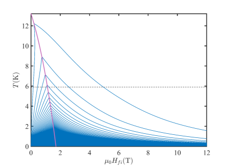
Figure 1: The $H-T$ instability diagram. The parameters employed to obtain this diagram are presented at the beginning of section IV. The purple line is the first penetration field $\mu_{0}H_{P}$ for different temperatures. The blue curves represent the instability field branches $\mu_{0}H_{fi,m}$ for $m=0,1,2,\dots$. As can be seen, as the temperature decreases, the branches tend to spliced. The dash black line denotes the temperature of the thermal bath $T_{B}=5.9\mathrm{K}$.

The $H-T$ instability diagram presented in the figure 1 is obtained via the equation (30) where the blue curves are the instability field branches $\mu_{0}H_{fi,m}$. Notice how the branches tend to spliced as the temperature decreases. This fact can related with the superconducting material behavior, it seems that at low temperatures it is unstable for any applied field value, consequently, the avalanches will always happen.

The PP and FP states are separated by the purple line which corresponds to the first penetration field $\mu_{0}H_{P}$, calculated with the equation (18), for different temperatures $T=T_{P}$. Each branch has a temperature range $(0,T_{p}]$, the branch $m=0$ for the PP state corresponds to the Wipf’s field, it is extended close to the superconducting transition temperature, and is the only one that presents a change of curvature.

The Wipf’s field is also defined for FP states, it is characterized by a change of curvature for temperatures close to $T_{P}$, this change can be related with the dominant influence of the thermal properties respect to the magnetic ones, due to its proximity to the superconducting transition temperature. For the rest of the branches, the magnetic properties will dominate. Even though the richness of this instability diagram, it is uncertain the exact applied field value where a flux jump occurs.

We retrieved from Chabanenko’s experiment, the applied magnetic field rate of $1\mathrm{T/min}\approx 0.02\mathrm{T/s}$, even so the step size was not reported, here it was estimated as $0.02\mathrm{T}$ with an error of $\pm 0.005$.

The dashed black line denotes the temperature of the thermal bath $T_{B}=5.9\mathrm{K}$. The $H-T$ diagram shows that for PP states the branches $m=0,1,2,3$ correspond to $\mu_{0}H_{P}>\mu_{0}H_{fi,m}=0.17;0.42;0.76;1.01\mathrm{T}$ respectively. For FP states the equation (36) has real solutions only for the branches $m=3,2,1,0$ which are $\mu_{0}H_{fi,m}=1.23;1.71;2.59;4.95\;\mathrm{T}$, respectively. The table 1 contains the above results as well as the experimental data of $\mu_{0}H_{fi,m}$.

The experimental magnetization curve presents three instability fields $\mu_{0}H_{fi}=0.45,1.09,2.61\mathrm{T}$ at the first quadrant. As can be appreciated, the fields $\mu_{0}H_{fi,1}=0.42\mathrm{T}$, $\mu_{0}H_{f,3}=1.01\mathrm{T}$ for states PP and $\mu_{0}H_{fi,1}=2.59\mathrm{T}$ for FP states are in good agreement with the experimental data.

As usual, the third quadrant of the curve is pretty similar to the first quadrant. In the third quadrant there are four instability fields $|\mu_{0}H_{fi}|=0.15,0.44,0.75,1.05\;\mathrm{T}$, they were estimated using a graphic digitalization procedure. The third instability field is an abrupt slope change of the curve rather than a conventional flux jump. The experimental and theoretical values almost match, such closeness suggests that indeed occurred an instability, however the flux jump was frustrated by some unknown physical mechanism.

Instability field $|\mu_{0}H_{fi}|\;\mathrm{(T)}$ at $5.9\mathrm{K}$
Theory($\mu_{0}H_{fi,m}$)			ExperimentChaba2013
Quadrant 1			Quadrant 1	Quadrant 3
m	PP	FP
0	0.17	4.95	0.45	0.15
1	0.42	2.59	1.09	0.44
2	0.76	1.71	2.61	0.75∗
3	1.01	1.22	-	1.05
PP: partial penetrate. FP: Full penetrate. (∗) This instability field is estimated where the magnetization curve has an abrupt change.

Table 1: Theoretical and experimental values of the instability field $\mu_{0}H_{fi,m}$

IV.2 Magnetic induction profiles

Once the external instability fields have been found, it is interesting to know the magnetic induction behavior. Figure 2 shows the magnetic induction of the superconducting material precisely at the instability field, also the isothermal as well as the disturbed fields are graphed. Panel (a): The black lines are the isothermal field distribution $B$, while the blue and red lines are the disturbed field corresponding to PP and FP states, respectively. Panels (b) and (c) show the $\Delta B$ oscillatory behavior, for PP and FP states respectively; to magnify $\Delta B$ it was used a perturbation amplitude $D=0.1(\mathrm{T})$.

The perturbed magnetic induction resembles a flexible cantilever structure with its fixed edge at the superconductor boundary, and maximum amplitude $D$. For PP states the oscillations increase as the instability field increases because the external field suffers a great opposition to diffuse into the superconducting material, unlike for FP states where occurs the opposite.

Although the graphs shape suggests that instability fields resonances may occur, it is important to point out that our theory exclude them, however the oscillations are only present at the instabilities. For another external field value, the magnetic induction will not suffer any deviation from its isothermal behavior.

The oscillations promote or inhibit the magnetization, this fact can be appreciated in panel (a). There are regions where the incursion of $B$ is encouraged and other ones where is mitigated, at this scenario, the current density magnitude can approach to zero once the temperature reaches its maximum value, while if the temperature decreases, the current density value is increased.

IV.3 Temperature change

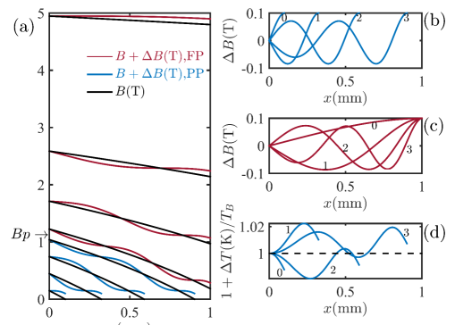
Figure 2: For a temperature $T_{B}=5.9\mathrm{K}$ and a penetration field $\mu_{0}H_{P}=1.12\mathrm{T}$ there are eight instability fields given by $\mu_{0}H_{fi,m}=B_{T}(2m+1)\pi/2+B_{H}$. For states PP $m=0,1,2,3$, then $\mu_{0}H_{fi,m}=0.17;0.42;0.76;1.01\mathrm{T}$, and for states FP, $m=3,2,1,0$ then $\mu_{0}H_{fi,m}=1.23;1.71;2.59;4.95\;\mathrm{T}$ (see table 1). Panel (a): the magnetic induction profiles $B+ΔB$ are shown, for PP they are the blue lines and for FP they are the red lines, while the black lines correspond only to $B$. Panels (b) and (c) show the behavior of the deviation $ΔB$ inside the sample for PP and FP states respectively. We used a perturbation amplitude $D=0.1(\mathrm{T})$ to magnify $\Delta B$. Panel (d) shows the change of temperature around the temperature of the thermal bath for PP states, using $D=0.0001(\mathrm{T})$ is obtained a maximum deviation of 2%.

This example finished with the description of the temperature. The theory describes a temperature change $\Delta T$ produced by Joule’s heat, in the adiabatic regime. This causes that the reference isothermal state becomes a non-equilibrium disturbed state. At this regime the temperature still be not homogeneous, this fact is illustrated by calculating $\Delta T$. Given the boundary condition $T(x=0)=T_{B}$, the local temperature is $T=T_{B}-\Delta T+\Delta T(x=0)$, and using the equations (22) and (29) for PP states, it is found the following:

$$T=T_{B}+\frac{\alpha}{\partial_{T}\alpha}\frac{D}{B_{T}}\left(1+\displaystyle\frac{B_{f}}{B^{*}}\right)^{\displaystyle\!\!n}\!\!\left(\frac{\mathrm{sgn}\left(\displaystyle\sin{\frac{B-B_{f}}{B_{T}}}\right)}{\left(1+\displaystyle\frac{\mu_{0}H_{if,m}}{B^{*}}\right)^{\displaystyle\!\!n}\!\!}-\frac{\displaystyle\sin{\frac{B-B_{f}}{B_{T}}}}{\left(1+\displaystyle\frac{B}{B^{*}}\right)^{\displaystyle\!\!n}\!\!}\right).$$

As is expected, the theory predicts for the temperature an oscillating flexible cantilever behavior, in the adiabatic regime. Panel (d) of figure 2 shows the temperature profile around the thermal bath temperature for PP states; employing the value $D=0.0001(\mathrm{T})$ is obtained a maximum deviation of 2%. The maximum temperature increment is determined by the intensity of the perturbation $D$, in our theoretical calculation we assume that it is a constant quantity but it must depend on the external field and the thermal properties of material.

V Conclusion

Starting from a simple but strong physical scheme the thermomagnetic stability of type-II superconductors is studied, this allows to find the instability field $H_{fi,m}$ for external magnetic fields applied with arbitrary direction at the $yz$ sample plane.

With this theory is possible to construct $H-T$ maps for both PP and FP states to accurately predict the instability field $H_{fi,m}$ according to the thermal bath and field applied values, this result marks differences from Wipf’s scheme PhysRev.161.404 since his approach was constrained to find the only one solution $H_{fi,0}$ for PP states, meanwhile in this work one can obtain a rich branches set for $H_{fi,m}$, going further up to FP states.

Since the theorical study is a first order approximation, the deviation behavior is periodic along the $x$ direction. It is constructed critical state magnetic induction profiles that resemble a flexible cantilever structures.

The instability field indicates a flux jump occurrence, and the theory presented here found that an ondulatory profile corresponds to a flux jump. Even so is not possible during an experiment to determine accurately the instability field value where a flux jump appears, if the step size $\Delta H$ is changed, there is a neighborhood around the theoretical value where can be detected a jump during the experiment. Thus it is reasonable to think that the oscillatory behavior can be replicated to profiles around the instability field.

There remains the challenging to consider an anisotropic critical state model0953-2048-26-12-125001 ; 0953-2048-29-4-045004 , both thermal and conductive properties of the heat capacity $C(T,H)$, as well as other sample geometryxia2017numerical .

Appendix A Temperature change $\Delta T$

The temperature change $\Delta T$ is obtained from the heat equation

$$C(T)\frac{dT}{dt}=\nabla\cdot(\alpha(T)\nabla T)+\frac{\partial Q}{\partial t},$$

integrating from time and assuming the adiabatic regime, where $\nabla\cdot(\alpha(T)\nabla T)\approx 0$ and $\partial_{t}C(T)\approx 0$, it is obtained that

$$C(T)\Delta T=\Delta Q,$$ (38)

here $\Delta Q$ corresponds to the heat change generated by the critical current density and the electromotive force produced by the magnetic induction profiles changes. To obtain an analytic expression for the heat change, we use the Faraday induction law as follows:

$$E_{z}=\int\frac{\partial B_{y}}{\partial t}dx+E_{z0},\quad E_{y}=-\int\frac{\partial B_{z}}{\partial t}dx+E_{y0}.$$

Substituting the former equations into Joule’s heat $dQ/dT=\mathbf{E}\cdot\mathbf{j}$, one has that

$$\frac{dQ}{dt}=-j_{y}\!\!\int\!\!\frac{\partial B_{z}}{\partial t}dx+j_{z}\!\!\int\!\!\frac{\partial B_{y}}{\partial t}dx+j_{y}E_{y0}+j_{z}E_{z0}$$

Employing the relations

$$j_{y}=j_{c}\cos{\varphi} j_{z}=j_{c}\sin{\varphi}$$

$$B_{y}=B\cos{\phi} B_{z}=B\sin{\phi}$$

we have that

$$\frac{dQ}{dt}=j_{c}\sin{(\varphi-\phi)}\int\frac{\partial B}{\partial t}dx+j_{c}(E_{y0}\cos\varphi+E_{z0}\sin\varphi)$$

The last term can be associated to the background heat produced by a constant voltage applied to the superconductor. In our study we assume that $E_{y0}=E_{z0}=0$, besides, the material is isotropic thus $\varphi=\phi+\pi/2$. With the above information, the heat change takes the final form:

$$\Delta Q = \int j_{c}\left(\int\frac{\partial B}{\partial t}dx\right)dt=j_{c}\int\!\!\Delta Bdx+\int\left(\int\frac{\partial B}{\partial t}dx\right)\frac{\partial j_{c}}{\partial t}dt,$$

$$\approx j_{c}\int\!\!\Delta Bdx,$$

where $\partial_{t}j_{c}\approx 0$. Finally, substituting the last equation into (38) we obtain:

$$\Delta TC(T)=j_{c}\int_{x}^{x_{0}}\!\!\Delta Bdx.$$

References

References

- (1) V Al’tov. Stabilization of superconducting magnetic systems. Springer Science & Business Media, 2013.
- (2) V. V. Chabanenko, S. V. Vasiliev, A. Nabiałek, A. S. Shishmakov, F. Pérez-Rodríguez, V. F. Rusakov, A. Szewczyk, B. N. Kodess, M. Gutowska, J. Wieckowski, and H. Szymczak. Boundaries of the critical state stability in a hard superconductor nb3al in the h–t plane. Low Temperature Physics, 39(4):329–337, 2013.
- (3) R Cortés-Maldonado, O De la Peña-Seaman, V García-Vázquez, and F Pérez-Rodríguez. On the extended elliptic critical-state model for hard superconductors. Superconductor Science and Technology, 26(12):125001, 2013.
- (4) N. D. Espinosa-Torres, J. F. J. Flores-Gracia, A. D. Hernández de la Luz, J. A. Luna-López, J. Martínez-Juárez, and G. Flores-Carrasco. Modeling the effect of thermal field in formation of magnetic flux avalanches in hard superconductors. Journal of Superconductivity and Novel Magnetism, 28(5):1507–1514, 2015.
- (5) Y. B. Kim, C. F. Hempstead, and A. R. Strnad. Magnetization and critical supercurrents. Phys. Rev., 129:528–535, Jan 1963.
- (6) V. Romanovskii. Temperature factor for magnetic instability conditions of type – {II} superconductors. Physica C: Superconductivity, 505:89 – 99, 2014.
- (7) C Romero-Salazar. Bianisotropic-critical-state model to study flux cutting in type-ii superconductors at parallel geometry. Superconductor Science and Technology, 29(4):045004, 2016.
- (8) C. Romero-Salazar and O. A. Hernández-Flores. Exploring solutions for Type-II superconductors in critical state. Revista Mexicana de Física, 59:123 – 130, 04 2013.
- (9) J Sosnowski. On the flux jumps in hard superconductors. physica status solidi (a), 79(1):207–212, 1983.
- (10) J. Sosnowski. Flux jumps in hard superconductors in decreasing magnetic field. Revue de Physique Appliquee, 20(4):221–224, 1985.
- (11) J Sosnowski. Influence of magnetic history on flux jump fields. Journal of applied physics, 59(12):4189–4191, 1986.
- (12) S. L. Wipf. Magnetic instabilities in type-ii superconductors. Phys. Rev., 161:404–416, Sep 1967.
- (13) SL Wipf. Review of stability in high temperature superconductors with emphasis on flux jumping. Cryogenics, 31(11):936–948, 1991.
- (14) Jing Xia, Maosheng Li, and You-He Zhou. Numerical investigations on the characteristics of thermomagnetic instability in mgb 2 bulks. Superconductor Science and Technology, 2017.
- (15) Ming Xu, Donglu Shi, and Ronald F. Fox. Generalized critical-state model for hard superconductors. Phys. Rev. B, 42:10773–10776, Dec 1990.