MOA-2016-BLG-319Lb: Microlensing Planet Subject to Rare Minor-Image Perturbation Degeneracy in Determining Planet Parameters

Abstract

We present the analysis of the planetary microlensing event MOA-2016-BLG-319. The event light curve is characterized by a brief ($\sim 3$ days) anomaly near the peak produced by minor-image perturbations. From modeling, we find two distinct solutions that describe the observed light curve almost equally well. From the investigation of the lens-system configurations, we find that the confusion in the lensing solution is caused by the degeneracy between the two solutions resulting from the source passages on different sides of the planetary caustic. These degeneracies can be severe for major-image perturbations but it is known that they are considerably less severe for minor-image perturbations. From the comparison of the lens-system configuration with those of two previously discovered planetary events, for which similar degeneracies were reported, we find that the degeneracies are caused by the special source trajectories that passed the star-planet axes at approximately right angles. By conducting a Bayesian analysis, it is estimated that the lens is a planetary system in which a giant planet with a mass $M_{\rm p}=0.62^{+1.16}_{-0.33}~{}M_{\rm J}$ ($0.65^{+1.21}_{-0.35}~{}M_{\rm J}$) is orbiting a low-mass M-dwarf host with a mass $M_{\rm h}=0.15^{+0.28}_{-0.08}~{}M_{\odot}$. Here the planet masses in and out of the parentheses represent the masses for the individual degenerate solutions. The projected host-planet separations are $a_{\perp}\sim 0.95$ au and $\sim 1.05$ au for the two solutions. The identified degeneracy indicates the need to check similar degeneracies in future analyses of planetary lensing events with minor-image perturbations.

1. Introduction

Microlensing signals of planets are often described by the phrase “a brief anomaly” to the lensing light curve produced by the host of the planet. However, this phrase is oversimplified because the pattern of planet-induced anomalies greatly varies depending on the configurations of lens systems. Furthermore, planetary signals in some cases of lens configurations can be confused with anomalies produced by other reasons and this induces a degeneracy problem in which multiple interpretations exist for an observed anomaly pattern. Therefore, identifying the origins of degeneracies in various lens configurations is important to find correct interpretations of microlensing planets by enabling one to check similar degeneracies in future analyses.

The degeneracies in the interpretation of planetary signals are broadly classified into two categories: “intrinsic” and “accidental”. The intrinsic degeneracies are caused by the symmetry of the lens equation, which describes the mapping from the source position on the lens plane into the image position on the source plane. The most well known of these is the “close/wide” degeneracy in which a pair of planetary models with projected separations from the host (normalized to the angular Einstein radius $\theta_{\rm E}$) $s$ and $s^{-1}$ result in very similar anomaly patterns. This degeneracy was first found by Griest & Safizadeh (1998) for a specific case of a planetary lens system and later extended to general binary lenses by Dominik (1999) and further investigated by An (2005).

Accidental degeneracies, on the other hand, occur due to the fortuitous alignment of lensing magnification patterns arising from unrelated lens configurations. It was pointed out by Gaudi (1998) that a subset of binary-source events, for which the flux ratio between the binary source stars is small and the lens approaches close to the faint source companion, can produce short-term anomalies, which are similar to those of planet-induced anomalies. These planet/binary-source degeneracies were actually found for MOA-2012-BLG-486 (Hwang et al., 2013) and OGLE-2015-BLG-1459 (Hwang et al., 2018c) for which the degeneracies were difficult to be resolved just based on the lensing light curves and could be resolved with additional data acquired from multi-band observations. Han & Gaudi (2008) pointed out another type of accidental degeneracies in which planetary signals can be imitated by those produced by binaries composed of roughly equal masses. Such degeneracies were demonstrated for OGLE-2011-BLG-0526, OGLE-2011-BLG-0950/MOA-2011-BLG-336 (Choi et al., 2012) and OGLE-2015-BLG-1212 (Bozza et al., 2016). In addition, incomplete coverage of the planet-induced anomalies can cause degeneracies in interpreting anomalies as demonstrated in the case of OGLE-2012-BLG-0455/MOA-2012-BLG-206 (Park et al., 2014; Hwang et al., 2018a).

Gaudi & Gould (1997) (hereafter GG1997) predicted another type of accidental degeneracy, in which two planetary lens configurations had similar $(s,q,\alpha)$ but with the source passing on different sides of the caustic. Here $q$ is the planet/host mass ratio and $\alpha$ represents the angle between the trajectory of the source and the axis connecting the planet and its host (source trajectory angle). Gould & Loeb (1992) argued that (under the assumption that the source passed directly over the caustic) one could read off the values of $(s,\alpha)$ from the three Paczyński (1986) parameters of the point-lens fit $(t_{0},u_{0},t_{\rm E})$ and the time of the planetary perturbation ($t_{\rm anom}$) using the relations

$$s-{1\over s}=\left(u_{0}^{2}+\tau_{\rm anom}^{2}\right)^{1/2};\qquad\tau_{\rm anom}={t_{\rm anom}-t_{0}\over t_{\rm E}},$$ (1)

and

$$\tan\alpha={u_{0}\over\tau_{\rm anom}}.$$ (2)

If the caustic is relatively small, this approach is approximately accurate, even if the source only passes near the caustic. However, GG1997 recognized that this would lead to two slightly different solutions depending on whether the source passes on one side of the caustic or the other. They pointed out that the degeneracy would be severe for perturbations produced by planets with projected planet-host separations greater than the angular Einstein radius ($s>1$, ‘wide’ planet): “major image perturbations”. For “minor-image perturbations”, which are produced by ‘close’ planets with $s<1$, on the other hand, it was thought that the degeneracy would be considerable less severe. This is mainly because of the qualitative difference in the caustic structures between the wide and close planetary systems, in which a wide planet induces a single set of planetary caustics and a close planet induces two sets. In Appendix, we review basic facts about the types of planetary anomalies caused by major and minor-image perturbations for readers who are not familiar with microlensing jargon. Experts will skip this appendix. For the major-image caustic, the magnification pattern on the near and far sides of the caustic are similar, and thus the anomalies produced by the source passing both sides of the caustic are similar to each other. For minor-image perturbations, on the other hand, the source trajectory passing the inner cusp will, in general, approach close to one of the two planetary caustics, while the source trajectory passing the outer cusp will approach the other caustic. As a result, the degeneracy would be generally resolvable from the presence (absence) and/or timing of the anomalies produced by the individual caustics.

Degeneracies involved with planetary caustics have been demonstrated for actual lensing events and new types of degeneracies are additionally found with the increasing number of microlensing planets. An example of the GG1997 degeneracy was recently found for the planetary event OGLE-2017-BLG-0173 (Hwang et al., 2018d), for which there existed 3 degenerate solutions and among them 2 solutions were caused by the degeneracy predicted by GG1997. We note that the other solution results from a new discrete degeneracy between the solution in which the caustic is fully enveloped (“Cannae” solution) and the solution in which only one side of the caustic is enveloped (“von Schlieffen” solution): “Hollywood” degeneracy. The two solutions resulting from the Hollywood degeneracy have different mass ratios because the source passes through the caustic in different places. Skowron et al. (2018) found a more specific case of GG1997 degeneracies from the analysis of the planetary lensing event OGLE-2017-BLG-0373. This so-called “caustic-chiral” degeneracy arises when the source passes over the caustic (contrary to the GG1997 degeneracy), but there are gaps in data. In this case, the solutions have very similar $(s,\alpha)$ but substantially different $q$. Another example of the caustic-chiral degeneracy was found by Hwang et al. (2018a) for KMT-2016-BLG-0212. In addition, there is a case of the source passing through a major-image caustic and being degenerate with passing through a minor-image caustic. This degeneracy was identified for KMT-2016-BLG-1107 by Hwang et al. (2018b).

In this work, we analyze the planetary event MOA-2016-BLG-319. The light curve is characterized by a short-term anomaly near the peak produced by the minor-image perturbation. Contrary to the expectation that interpreting minor-image perturbations would not suffer from degeneracies, we find two discrete solutions that describe the observed light curve almost equally well. Similar degeneracies in minor-image perturbations were reported for two planetary events OGLE-2016-BLG-1067 (Calchi Novati et al., 2018b) and OGLE-2012-BLG-0950 (Koshimoto et al., 2017). By analyzing the similarity between the anomalies of the events, we investigate the origin of the degeneracy.

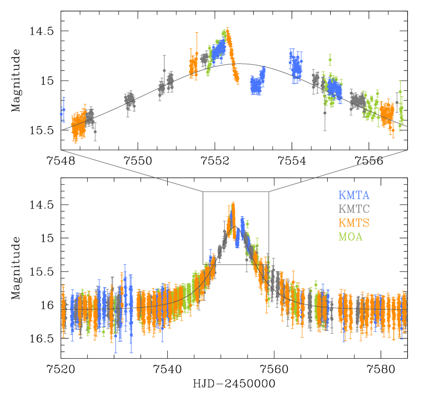
Figure 1.— Light curve of the lensing event MOA-2016-BLG-319. The zoom of the anomaly near the peak is shown in the upper panel. Superposed on the data points represents the point-source point-lens model.

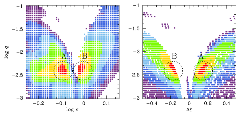
Figure 2.— $\Delta\chi^{2}$ distributions of points in the MCMC chain on the $\log s$–$\log q$ (left panel) and $\Delta\xi$–$\log q$ (right panel) planes. The parameter $q$ denotes the planet/host mass ratio, $s$ is the projected planet-host separation, and $\Delta\xi$ represents the separation between the source and the planetary caustic at the time of the anomaly. Points marked in different colors represents those in the MCMC chain with $<10\sigma$ (red), $<20\sigma$ (yellow), $<30\sigma$ (green), $<40\sigma$ (cyan), $<50\sigma$ (blue), and $<60\sigma$ (purple).

2. Observations

We identify the case of degeneracies in minor-image perturbations from the analysis of the lensing event MOA-2016-BLG-319. Figure 1 shows the event light curve. The source star of the event is located at the Galactic bulge field with equatorial coordinates $({\rm RA},{\rm DEC})_{\rm J2000}=(17:54:58.13,-29:45:01.67)$. The corresponding galactic coordinates are $(l,b)=(0.35^{\circ},-2.17^{\circ})$. The magnification of the source star induced by lensing was first detected and announced to microlensing community on 2016 June 13, ${\rm HJD}^{\prime}={\rm HJD}-2450000\sim 7552$, by the Microlensing Observations in Astrophysics (MOA) survey (Bond et al., 2001; Sumi et al., 2003). The MOA survey used the 1.8 m telescope located at Mt. John Observatory, New Zealand. The day of the event alert approximately corresponds to not only the time of the light curve peak but also the start of a short-term anomaly, which lasted for $\sim 3$ days during $7551.5\lesssim{\rm HJD}^{\prime}\lesssim 7554.5$. However, it was difficult to notice the anomaly because the MOA survey could not cover the event for 4 consecutive nights before the anomaly and the photometry of data during the anomaly was not good enough to delineate the anomaly pattern. As a result, little attention was paid to the event during the progress of the event.

The scientific importance of the event was noticed with the additional data acquired by Korea Microlensing Telescope Network (KMTNet) survey (Kim et al., 2016) conducted using three 1.6 m telescopes. The individual KMTNet telescopes are positioned at the Cerro Tololo Interamerican Observatory, Chile (KMTC), the South African Astronomical Observatory, South Africa (KMTS), and the Siding Spring Observatory, Australia (KMTA). The alert system of the KMTNet survey started from the 2018 season (Kim et al., 2018b) and the progress of the event was not known in real time at the time of the event during the 2016 season. From the analysis of lensing events identified by applying the Event Finder algorithm (Kim et al., 2018a, b) to the 2016 season data, it was found that KMTNet data densely covered the light curve peak which clearly showed a short-term anomaly. See the zoom of the light curve around the anomaly region presented in the upper panel of Figure 1. The event was identified by KMTNet as KMT-2016-BLG-1816.

Table 1Data sets used in the analysis

Data set	Range	$N_{\rm data}$
MOA	$7502\lesssim{\rm HJD}^{\prime}\lesssim 7569$	757
KMTA (BLG02)	$7440\lesssim{\rm HJD}^{\prime}\lesssim 7676$	798
KMTA (BLG42)	$7443\lesssim{\rm HJD}^{\prime}\lesssim 7676$	701
KMTC (BLG02)	$7439\lesssim{\rm HJD}^{\prime}\lesssim 7675$	1143
KMTC (BLG42)	$7439\lesssim{\rm HJD}^{\prime}\lesssim 7675$	1006
KMTS (BLG02)	$7441\lesssim{\rm HJD}^{\prime}\lesssim 7681$	1394
KMTS (BLG42)	$7441\lesssim{\rm HJD}^{\prime}\lesssim 7681$	1472

Note. — ${\rm HJD}^{\prime}={\rm HJD}-2450000$.

In Table 1, we present the data sets used in the analysis. MOA observations of the event was conducted in a customized $R$ band with a cadence of 1 hr. KMTNet observations were conducted mostly in $I$ band with occasional observations in $V$ band to measure the source color. The event was in the KMTNet BLG02 and BLG42 fields which were monitored with a cadence of 0.5 hr by the individual telescopes. For the period from April 23 (${\rm HJD}^{\prime}\sim 2457501$) to June 16 (${\rm HJD}^{\prime}\sim 2457555$), the cadence of KMTS and KMTA was increased in order to support Kepler K2 C9 campaign (Gould & Horne, 2013). While the event does not lie in the K2 field, the anomaly coverage serendipitously benefited from this cadence increase. The columns ‘range’ and ‘$N_{\rm data}$’ indicate the time range of the data sets used for analysis and the number of data points constituting the individual data sets, respectively. We set the range of the MOA data in the region around event because the baseline data exhibit considerable fluctuation.

Photometry of data are processed using the codes of the individual groups: Bond et al. (2001) for the MOA survey and Albrow et al. (2009) for the KMTNet survey. Both codes utilize the difference imaging method developed by (Alard & Lupton, 1998). Errorbars are normlized using the recipe explained in Yee et al. (2012).

3. Light curve Analysis

The light curve shows a pronounced dip. Such a dip feature in lensing light curves can only be produced by minor image perturbations. There are two possibilities in the lens-system configuration. First, minor image gives rise to two triangular planetary caustics with a magnification dip between them. Second, there is a six-sided resonant caustic whose “back end” consists of two caustic wings separated by a dip. See Figure 4 of Gaudi (2012) for the variation of planetary microlens caustics.

Although some lens configurations are excluded in advance based on the previously well-studied origins of degeneracies, interpreting the anomaly may be subject to unknown types of degeneracies. We, therefore, conduct a thorough grid search for the planetary lensing parameters $s$ and $q$. Besides these planetary parameters, one needs additional lensing parameters to model the observed light curve. These parameters describe the source star’s approach to the lens including the time of the closest approach, $t_{0}$, the lens-source separation at that time, $u_{0}$ (impact parameter), the event time scale, $t_{\rm E}$ (Einstein time scale), and the source trajectory angle. The anomaly might be produced by the crossings of the source over caustics. There is no obvious signature of caustic crossings, which usually produce sharp spike feature. However, caustic-crossing features can be smooth if the source is substantially bigger than the caustic. Even if a source is smaller than an overall caustic, it could be big compared to the caustic figure that it is passing over, e.g., OGLE 2016-BLG-1195 (Bond et al., 2017) and OGLE-2016-BLG-1195 (Shvartzvald et al., 2017). These finite-source effects were theoretically predicted by Bennett & Rhie (1996) and observationally confirmed by Beaulieu et al. (2006) for the planetary lensing event OGLE-2005-BLG-390. To account for possible finite-source effects, we include an additional parameter of the normalized source radius $\rho$, which denotes the ratio of the angular source radius $\theta_{*}$ to the angular Einstein radius $\theta_{\rm E}$, i.e., $\rho=\theta_{*}/\theta_{\rm E}$. For a given set of the planetary parameters $s$ and $q$, we search for the other parameters using the Markow Chain Monte Carlo (MCMC) method. We set the ranges of the grid parameters, i.e., $s$ and $q$, wide enough to check the possibility that the anomaly is produced by binaries that have similar mass components.

In the left panel of Figure 2, we present $\Delta\chi^{2}$ distribution of points in the MCMC chain on the $\log s$–$\log q$ plane acquired from the preliminary grid search. From the distribution, one first finds that the lens responsible for the anomaly is composed of two masses with a very low mass ratio of $q\sim 4\times 10^{-3}$, suggesting that the lower-mass component of the lens is a planet. One also finds that there exist two distinct solutions centered at $(\log s,\log q)\sim(-0.09,-2.4)$ (marked by “A”) and $\sim(-0.02,-2.4)$ (“B”). From further refinement of the individual local solutions by letting all parameters vary, it is found that the $\chi^{2}$ difference between the two solutions is merely $\Delta\chi^{2}\sim 1.9$. This indicates that both solutions describe the observed anomaly almost equally well, although the solution “A” is slightly preferred over the solution “B”.

Table 2Best-fit lensing parameters

Parameter	Inner solution (“A”)	Outer solution (“B”)
$\chi^{2}$	7308.1	7310.0
$t_{0}$ (HJD′)	7552.737 $\pm$ 0.013	7552.742 $\pm$ 0.012
$u_{0}$	0.267 $\pm$ 0.012	0.260 $\pm$ 0.012
$t_{\rm E}$ (days)	8.60 $\pm$ 0.26	8.69 $\pm$ 0.26
$s$	0.817 $\pm$ 0.004	0.945 $\pm$ 0.008
$q$ ($10^{-3}$)	3.93 $\pm$ 0.11	4.10 $\pm$ 0.12
$\alpha$ (rad)	4.646 $\pm$ 0.006	4.645 $\pm$ 0.006
$F_{\rm s,KMTC}$	6.25 $\pm$ 0.08	6.23 $\pm$ 0.08
$F_{\rm b,KMTC}$	-0.10 $\pm$ 0.11	-0.10 $\pm$ 0.11

Note. — ${\rm HJD}^{\prime}={\rm HJD}-2450000$.

To be noted is that the degeneracy between the two solutions is different from the previously known ‘close/wide’ degeneracy. The two solutions resulting from the close/wide degeneracy have planet-host separations $s$ and $s^{-1}$ and thus one solution has a separation smaller than $\theta_{\rm E}$, i.e., $s<1$, and the other solution has a separation greater than $\theta_{\rm E}$, $s>1$. In the case of MOA-2016-BLG-319, both degenerate solutions have separations $s<1$ ($s\sim 0.82$ for the solution “A” and $s\sim 0.95$ for the solution “B”) indicating that the origin of the degeneracy does not stem from the symmetry of the lens equation.

In Table 2, we present the best-fit lensing parameters for the two degenerate solutions. We also present the $\chi^{2}$ values of the fit for the solutions. The uncertainties of the parameters correspond to the scatter of points in the MCMC chain. We note that the lensing parameters of the two degenerate solutions are very similar to each other except for the binary separation $s$. To be also noted is that the time scale of the event, $t_{\rm E}\sim 8.6$ days, is short. As a result, higher-order effects induced by the orbital motion of the Earth, microlens-parallax effect (Gould, 1992), or that of the lens, lens-orbital effect (Dominik, 1998), is not important in describing the observed light curve. Also presented in the table are the flux values of the source, $F_{\rm s,KMTC}$, and blend, $F_{\rm b,KMTC}$, as measured from the pyDIA photometry of the KMTC data set. We note that the blend flux has a slightly negative value but it is consistent to be zero within the measurement error. These measured values of $F_{\rm s,KMTC}$ and $F_{\rm b,KMTC}$ indicate that the flux from the source dominates the blended flux.

In Figure 3, we present model light curves for both solutions plotted over the observed data points. Except for the very short period around ${\rm HJD}^{\prime}\sim 7553.4$, the two model light curves are so similar to each other that it is difficult to distinguish them within the line width, indicating that the degeneracy between the two solutions is very severe. This can be also seen in the lower two panels in which the residuals from the individual solutions are presented.

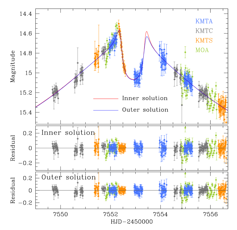
Figure 3.— Two model light curve resulting from the two degenerate solutions: “inner solution” and “outer solution”. The lower panels show the residuals from the individual solutions. The lens-system configurations corresponding to the individual solutions are presented in Fig. 4.

Figure 4 shows the configurations of the lens system for the individual solutions. In each panel, the line with an arrow represents the source trajectory, the small dots marked by $M_{1}$ and $M_{2}$ indicate the positions of the lens components, and the closed figures composed of concave curves represent the caustic. The upper and lower panels are the configurations for the solutions “A” and “B”, respectively. We draw contours of magnification to show the region of anomaly around the caustics. For the solution “A”, the caustic is composed of 3 sets in which the small caustic located close to the host is the central caustic and the two caustics located away from the host are the planetary caustics. According to this solution, the anomaly was produced by the passage of the source through the region between the central and planetary caustics. The negative deviation of the anomaly was produced during the time when the source passed the negative perturbation region between the central and planetary caustics. Because the source trajectory passed the inner region of the planetary caustic with respect to the planet host, we refer to this solution as “inner solution”. For solution “B”, on the other hand, the lens system produces a single resonant caustic. This results from the merging of the central and planetary caustics because of the proximity of the planet-host separation to unity, $s\sim 0.95$. According to this solution, the source trajectory passed the back-end of the caustic and the negative deviation occurred during the time when the source passed the region extending from the caustic end. Because the source trajectory passed the outer region of the caustic (with respect to the planet host), we refer to this solution as “outer solution”.

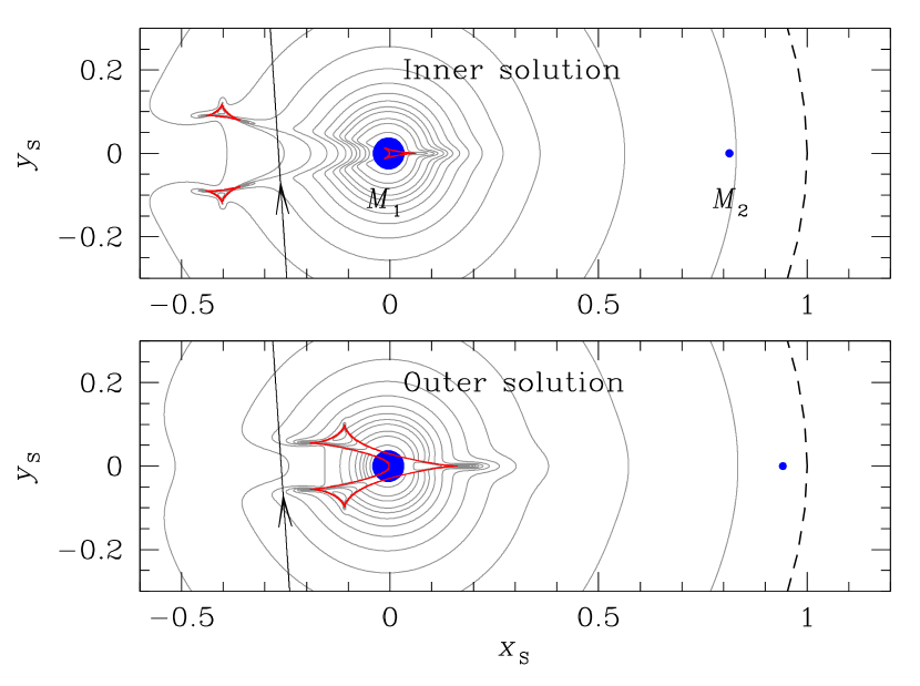
Figure 4.— Lens-system configurations for the two degenerate solutions seen on the source plane. For each panel, the curve with an arrows represents the source trajectory and the red closed curves represent caustics. The two dots marked by $M_{1}$ and $M_{2}$ denote the lens components, where $M_{1}>M_{2}$. The dashed circle centered at $M_{1}$ represents the Einstein ring. Contours of lensing magnification are drawn to show the region of anomaly around caustics.

For better understanding the origin of the degeneracy between the two solutions, in Figure 5, we present the lens-system configurations seen on the lens plane. In the plot, the planet host is located at the origin and the line with an arrow represents the path of the source. The two solid curves with arrows represent the paths of the images produced by the host. The red and blue dots represent the planet positions for the inner and outer solutions, respectively. From the configurations, it is found that, for both solutions, the planet is located close to the minor image produced by the host at the time of the perturbation. The difference in the configurations between the two solutions is that the planet is located inside the minor image (with respect to the host) for the “inner solution”, while it is located outside of the image for the “outer solution”. This indicates that the similarity between the two solutions is caused by the degeneracy in minor-image perturbations. We note that the lens system configuration is similar to that presented in Figure 1 of GG1997 except that the positions of planets are different.

The fact that the two solutions are originated from the GG1997 degeneracy can also be seen in the right panel of Figure 2, in which we plot $\Delta\chi^{2}$ distribution of MCMC points on the $\Delta\xi$–$\log q$ plane. Here $\Delta\xi$ represents the separation between the source and the planetary caustic at the time of the anomaly. The separation $\Delta\xi$ is determined from the lensing parameters by

$$\Delta\xi={u_{0}\over\sin\alpha}-\left(s-{1\over s}\right),$$ (3)

where the former term on the right side, i.e., $u_{0}/\sin\alpha$, represents the separation between the source and planet host at the time of the anomaly and the latter term, i.e., $s-1/s$, denotes the separation between the caustic center and the host. We note that similar plots are presented in Figure 4 of Hwang et al. (2018d) and Figure 5 of Skowron et al. (2018). From the plot, it is found that the degenerate solutions have similar separations $|\Delta\xi|\sim 0.15$ but with opposite signs, indicating that the source stars of the individual solutions approach the opposite sides of the caustic with similar separations from the caustic.

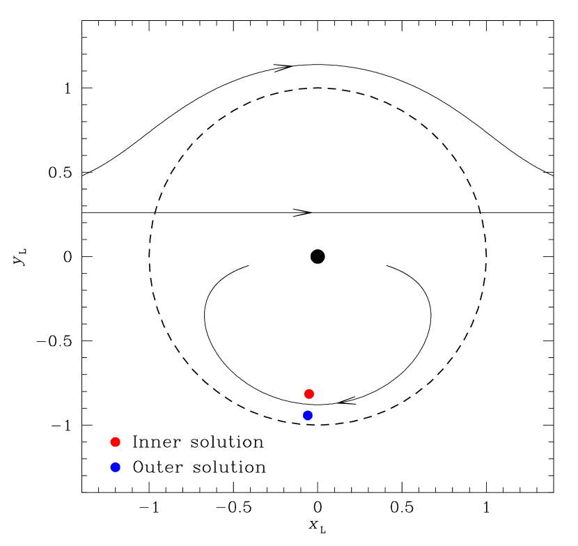
Figure 5.— Lensing system configurations for the two degenerate solutions seen on the lens plane. The coordinates are centered at the position of the planet host (black dot) and the dashed circle represents the Einstein ring. The solid line with an arrow represents the path of the source. The two solid curves with arrows represent the paths of the images produced by the planet host. The red and blue dots represent the planet positions for the inner and outer solutions, respectively.

Despite that degeneracies are thought to be considerably less severe for minor-image perturbations compared to major-image perturbations, similar degeneracies in minor-image perturbations were reported by Calchi Novati et al. (2018b) and Koshimoto et al. (2017) for the planetary events OGLE-2016-BLG-1067 and OGLE-2012-BLG-0950, respectively. We, therefore, compare the lens-system configurations of MOA-2016-BLG-319 with the two other events in order to find the cause of the degeneracy. The lens-system configurations of OGLE-2016-BLG-1067 are presented in Figures 3 and 4 of Calchi Novati et al. (2018b). We note that they presented 8 degenerate configurations, among which a four-fold degeneracy is caused by the space-based parallax measurement (Refsdal, 1966; Gould, 1994) and the other two-fold degeneracy is relevant to the minor-image perturbation. The configurations of OGLE-2012-BLG-0950 are presented in Figure 2 of Koshimoto et al. (2017).

From comparing the lens-system configurations of the events, we find one major difference and one major similarity. The difference is that the planetary caustics of the outer solution is separated from the central caustic for OGLE-2016-BLG-1067, while it is merged with the central caustic for MOA-2016-BLG-319 and OGLE-2012-BLG-0950 (resonant topology). However, in the sense that the source trajectory of MOA-2016-BLG-319 and OGLE-2012-BLG-0950 passed the planetary wing of the resonant caustic, the degeneracies of the events are considered to be of the same type. The similarity is that the source stars of the events passed the planet-host axes at about right angles. The source trajectory angles are $\alpha\sim 267^{\circ}$, $\sim 278^{\circ}$, $\sim 292^{\circ}$ for MOA-2016-BLG-319, OGLE-2016-BLG-1067, and OGLE-2012-BLG-0950, respectively. For general cases in which the entrance angle of the source is substantially different from a right angle, the source trajectory passing the inner region of the minor-image caustic produces a light curves that is distinct from a trajectory passing the outer region. On one side of the set of caustics, they will pass closer to one of the two caustics and farther from the other caustic. On the other side, the order will be inverted (for fixed angle). This will result in different anomaly patterns, and thus one can easily distinguish the two cases if the anomaly is densely covered. In the case of a right angle source entrance, on the other hand, the source approaches the individual caustics with approximately same distances. Then, the anomaly patterns resulting from the source trajectories passing the inner and outer regions of the planetary caustic can appear to be similar. We, therefore, conclude that the degeneracies in the minor-image perturbations of both events occur because the source stars crossed the star-planet axes at approximately right angles.

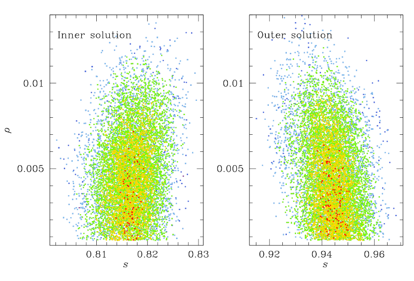
Figure 6.— Distributions of $\Delta\chi^{2}$ of points in the MCMC chain on the $s$–$\rho$ parameter plane. Color coding represents points within $1\sigma$ (red), $2\sigma$ (yellow), $3\sigma$ (green), $4\sigma$ (cyan), and $5\sigma$ (blue). The left and right panels are the distributions for the inner and outer solutions, respectively.

4. Source star

We characterize the source star based on the source flux measured in $I$ and $V$ passbands. Besides simply knowing the type of the source star, characterizing the source star is important because it may provide information about the angular Einstein radius in combination with the normalized source radius $\rho$ via the relation $\theta_{\rm E}=\theta_{*}/\rho$. For MOA-2016-BLG-319, however, the normalized source radius $\rho$ cannot be measured because deviations in the lensing light curve caused by finite-source effects cannot be firmly detected. See Figure 6, in which we plot the $\Delta\chi^{2}$ distributions of points in the MCMC chain on the $s$–$\rho$ parameter plane. However, the upper limit on $\rho$ can be measured and this yields a lower limit on $\theta_{\rm E}$, which may provide a constraint on the physical lens parameters. It is found that the upper limit of the normalized source radius is $\rho_{\rm max}\sim 0.01$ as measured at the $3\sigma$ level.

The de-reddened color $(V-I)_{0}$ and brightness $I_{0}$ of the source star are estimated using the known values of the red giant clump (RGC) centroid, $(V-I,I)_{{\rm RGC},0}=(1.06,14.41)$ (Bensby et al., 2011; Nataf et al., 2013), and the offsets in color and magnitude of the source from the RGC centroid. In Figure 7, we mark the positions of the source and RGC centroid in the color-magnitude diagram of stars located in the same field of the source. The positions of the source and the RGC centroid are $(V-I,I)=(2.00\pm 0.04,19.01\pm 0.01)$ and $(V-I,I)_{\rm RGC}=(2.29,15.94)$, respectively. From the color and brightness offsets, it is found that the de-reddened color and brightness of the source star are $(V-I,I)_{0}=(0.77\pm 0.04,17.49\pm 0.01)$, respectively. The estimated de-reddened color and magnitude of the source star indicate that the source is likely to be a turnoff star. We then convert the measured $V-I$ color into $V-K$ color using the $(V-I)/(V-K)$ relation of Bessell & Brett (1988). Finally, we estimate the source angular radius using the $(V-K)/\theta_{*}$ relation of Kervella et al. (2004). The estimated angular source radius is

$$\theta_{*}=1.07\pm 0.09\ \mu{\rm as}.$$ (4)

With the measured angular source radius, the lower limit of the angular Einstein radius is set to be

$$\theta_{\rm E,min}={\theta_{*}\over\rho_{\rm max}}\sim 0.107~{}{\rm mas}.$$ (5)

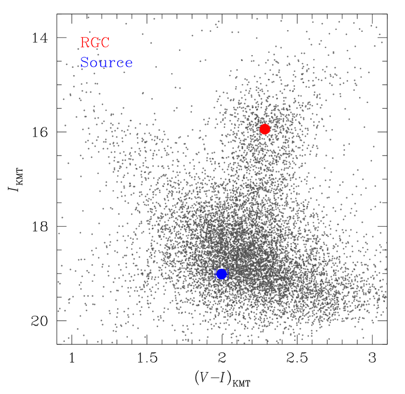
Figure 7.— Position of the source star in the instrumental color-magnitude diagram constructed based on the KMTNet data. Also marked is the location of red giant clump (RGC) centroid.

5. Bayesian Analysis of Lens Parameters

In order to uniquely determine the mass, $M$, and distance to the lens, $D_{\rm L}$, it is required to measure both the microlens parallax $\pi_{\rm E}$ and the angular Einstein radius $\theta_{\rm E}$, from which $M$ and $D_{\rm L}$ are determined by

$$M={\theta_{\rm E}\over\kappa\pi_{\rm E}};\qquad D_{\rm L}={{\rm au}\over\pi_{\rm E}\theta_{\rm E}+\pi_{\rm S}}$$ (6)

(Gould, 2000b). Here $\kappa=4G/(c^{2}{\rm au})\sim 8.14~{}{\rm mas}~{}M_{\odot}^{-1}$ and $\pi_{\rm S}={\rm au}/D_{\rm S}$ denotes the parallax of the source located at a distance $D_{\rm S}$. For MOA-2016-BLG-319, however, neither $\pi_{\rm E}$ nor $\theta_{\rm E}$ is measured, although the upper limit of $\theta_{\rm E}$ is set. We, therefore, conduct a Bayesian analysis of Galactic lensing events to estimate $M$ and $D_{\rm L}$ based on the measured event time scale. The time scale provides a constraint on the lens parameters because it is related to the parameters by

$$t_{\rm E}={\sqrt{\kappa M\pi_{\rm rel}}\over\mu};\qquad\pi_{\rm rel}={\rm au}\left({1\over D_{\rm L}}-{1\over D_{\rm S}}\right).$$ (7)

Here $\mu$ represents the relative lens-source proper motion. We also use the constraint of $\theta_{\rm E,min}$.

Implementing a Bayesian analysis requires models describing how lens objects are distributed, i.e., physical distribution, and how they move, i.e., dynamical distribution. One also needs a model mass function of lens objects. We construct the lens mass function based on the Chabrier (2003) mass function for stars combined with the Gould (2000a) mass function for stellar remnants including black holes, neutron stars, and white dwarfs. Lens and source objects are assumed to be distributed following the physical matter distribution model of Han & Gould (2003), in which the disk has a double-exponential form and the bulge has a triaxial shape. For the dynamical distribution, we adopt Han & Gould (1995) model, in which the motion of disk objects follows a gaussian velocity distribution with a mean corresponding to the rotation speed of the disk, and the motion of bulge objects follows a triaxial gaussian distribution with the velocity components along the individual axes deduced from the bulge shape via the tensor virial theorem. Based on the model distributions, we conduct a Monte Carlo simulation to generate a large number ($6\times 10^{6}$) of Galactic lensing events. Then, the the lens mass and distance distributions are constructed based on the events with time scales located within the range of the measured event time scale. With these distributions, we then estimate the representative values of $M$ and $D_{\rm L}$ as the median values. The lower and upper limits of the values are estimated as the 16% and 84% of the distribution.

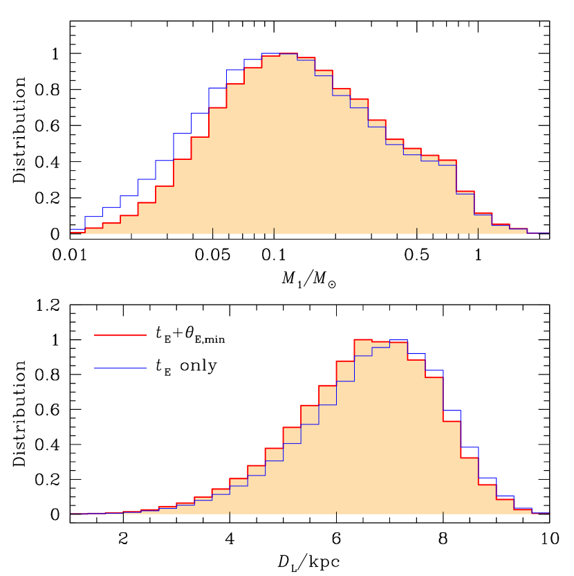
Figure 8.— Probability distributions of the mass (upper panel) and distance (lower panel) of the planet host. The blue curve is the distribution based on only the event time scale $t_{\rm E}$, while the red curve is the distribution with the additional constraint of the lower limit of the angular Einstein radius, $\theta_{\rm E,min}$.

In Figure 8, we present the distributions of the lens mass (upper panel) and distance (lower panel) obtained from the Bayesian analysis. In each panel, the blue curve is the distribution based on only the event time scale $t_{\rm E}$, while the red curve is the distribution obtained with the additional constraint of $\theta_{\rm E,min}$. It is found that the constraint of $\theta_{\rm E,min}$ is weak and thus has little effect on the probability distribution. The estimated masses of the lens components are

$$M_{1}=0.15^{+0.28}_{-0.08}~{}M_{\odot}$$ (8)

and

$$M_{2}=0.62^{+1.16}_{-0.33}~{}M_{\rm J}.$$ (9)

Therefore, the lens is a planetary system in which a giant planet is orbiting a low-mass M dwarf. Planetary systems belonging to low-mass hosts are difficult to be detected by other major planet detection methods, e.g., radial velocity or transit methods, due to the faintness of host stars. On the other hand, the microlensing method does not rely on the brightness of the host star, and thus the majority of planetary systems with low-mass stars were found using the microlensing method. See Figure 10 of Han (2018) and Figure 6 of Jung et al. (2018), which show the distribution of planets in the $M_{1}$–$M_{2}$ plane. The planetary system is estimated to be located at a distance of

$$D_{\rm L}=6.8^{+1.2}_{-1.4}~{}{\rm kpc}.$$ (10)

In Table 3, we list the physical lens parameters. We note that the ranges of the lens mass and distances are considerable due to the Bayesian nature of determining the lens parameters combined with weak constraint of extra information, e.g., $\theta_{\rm E}$ or $\pi_{\rm E}$. Also presented in the table is the projected separation between the planet and host, which is estimated by $a_{\perp}=sD_{\rm L}\theta_{\rm E}$. The projected separation is $a_{\perp}\sim 0.95$ au and $\sim 1.05$ au for the inner and outer solutions, respectively. In both cases, the planet is located away from the snow line at $a_{\rm snow}\simeq 2.7~{}{\rm au}(M/M_{\odot})\sim 0.4~{}{\rm au}$.

Table 3Physical Lens Parameters

Parameter	Inner solution	Outer solution
$M_{1}$ ($M_{\odot}$)	$0.15^{+0.28}_{-0.08}$	$0.15^{+0.28}_{-0.08}$
$M_{2}$ ($M_{\rm J}$)	$0.62^{+1.16}_{-0.33}$	$0.65^{+1.21}_{-0.35}$
$D_{\rm L}$ (kpc)	$6.8^{+1.2}_{-1.4}$	$6.8^{+1.2}_{-1.4}$
$a_{\perp}$ (au)	$0.95^{+0.17}_{-0.20}$	$1.09^{+0.19}_{-0.22}$

6. Summary

We presented the analysis of the planetary lensing event MOA-2016-BLG-319 for which the light curve was characterized by a short-term anomaly near the peak produced by the minor-image perturbation. From modeling of the light curve, we found that there existed two distinct solutions that described the observed light curve almost equally well. The planet-host separations of both solutions were smaller than the Einstein radius, indicating that the degeneracy was different from the previously known ‘close/wide’ degeneracy. From the investigation of the lens-system configurations, it was found that the two solutions resulted from the degeneracy in minor-images perturbations. Because it had been believed that the degeneracy in determining the planet parameters would not be severe for minor-image perturbations, such a degeneracy was unexpected. From the comparison of the lens-system configuration with those of OGLE-2016-BLG-1067 and OGLE-2012-BLG-0950, for which similar degeneracies were reported, we found that the degeneracies for the events were caused by the special source trajectories that passed the star-planet axis at approximately right angles. By conducting a Bayesian analysis, we estimated that the lens was a planetary system in which a giant planet with a mass $M_{\rm p}=0.62^{+1.16}_{-0.33}~{}M_{\rm J}$ ($0.65^{+1.21}_{-0.35}~{}M_{\rm J}$) was orbiting a low-mass M dwarf with a mass $M_{\rm h}=0.15^{+0.28}_{-0.08}~{}M_{\odot}$, where the planet masses in and out of the parentheses represent the masses for the inner and outer solutions, respectively. The projected host-planet separations were $a_{\perp}\sim 0.95$ au and $\sim 1.05$ au for the individual degenerate solutions. The identified degeneracy indicated the need to check similar degeneracies in future analysis of planetary events with minor-image perturbations.

Appendix A Types of Planetary Perturbations

When a source star is microlensed, the image of the source splits into two. One image with a higher magnification (“major image”) appears outside the Einstein ring and the other image with a lower magnification (“minor image”) appears inside the ring. Planetary perturbations occur at the time when the planet is positioned near one of the two microlens images of the primary star and additionally perturbs the nearby image (Mao & Paczyński, 1991; Gould & Loeb, 1992).

Depending on which image is perturbed by the planet, planetary perturbations are classified into two types: “major-image perturbation” and “minor-image perturbation” (GG1997). The major-image perturbation indicates the case in which the major image is perturbed by the planet. Because the major image is located outside the Einstein ring, major-image perturbations are caused by planets with separations $s>1$. On the other hand, minor-image perturbation indicates the case in which the minor image is perturbed by the planet. The minor image is located inside the Einstein ring and thus minor-image perturbations are caused by planets with separations $s<1$. When a major image is perturbed, the image is further magnified by the planet and thus the lensing light curve always exhibits positive deviations from the light curve produced by the host. In contrast, the minor-image perturbation causes the demagnitification of the image, producing, in most cases, a negative deviation in the light curve.

In the view point on the source plane, planetary lensing signals are produced when a source approaches the caustic produced by the planet. Planets induce one or two sets of “planetary caustics” depending on whether the planetary separation is greater or smaller than the Einstein radius. For the lens system with a wide planet, there exists a single set of planetary caustics with four cusps. For the system with a close planet, on the other hand, there exist two sets of caustics in which one is located above the planet-host axis and the other is located below the axis and each of the caustics is composed of three cusps. For the detailed properties of planetary caustics, see Han (2006).

References

- Alard & Lupton (1998) Alard, C., & Lupton, R. H. 1998, ApJ, 503, 325
- Albrow et al. (2009) Albrow, M. D., Horne, K., Bramich, D. M., et al. 2009, MNRAS, 397, 2099
- An (2005) An, J. H. 2005, MNRAS, 356, 1409
- Beaulieu et al. (2006) Beaulieu, J.-P., Bennett, D. P., Fouqué, P. 2006, Nature, 439, 437
- Bennett & Rhie (1996) Bennett, D. P., & Rhie, S. H. 1996, ApJ, 472, 660
- Bensby et al. (2011) Bensby, T., Adén, D., Meléndez, J., et al. 2011, PASP, 533, 134
- Bessell & Brett (1988) Bessell, M. S., & Brett, J. M. 1988, PASP, 100, 1134
- Bond et al. (2001) Bond, I. A., Abe, F., Dodd, R. J., et al. 2001, MNRAS, 327, 868
- Bond et al. (2017) Bond, I. A., Bennett, D. P., Sumi, T., et al. 2017, MNRAS, 469, 2434
- Bozza et al. (2016) Bozza, V., Shvartzvald, Y., Udalski, A., et al. 2016, ApJ, 820, 79
- Calchi Novati et al. (2018b) Calchi Novati, S., Suzuki, D., Udalski, A., et al. 2018b, arXiv: 1801.05806
- Chabrier (2003) Chabrier, G. 2003, ApJ, 586, L133
- Choi et al. (2012) Choi, J.-Y., Shin, I.-G., Han, C., et al. 2012, ApJ, 756, 48
- Chung et al. (2005) Chung, S.-J., Han, C., Park, B.-G., et al. 2005, ApJ, 630, 535
- Dominik (1998) Dominik, M. 1998, A&A, 329, 361
- Dominik (1999) Dominik, M. 1999, A&A, 349, 10
- Gaudi (1998) Gaudi, B. S. 1998, ApJ, 506, 533
- Gaudi (2012) Gaudi, B. S., 2012, ARA&A, 50, 411
- Gaudi & Gould (1997) Gaudi, B. S., & Gould, A. 1997, ApJ, 486, 85
- Gould (1992) Gould, A. 1992, ApJ, 392, 442
- Gould (1994) Gould, A. 1994, ApJ, 421, L75
- Gould (2000a) Gould, A. 2000a, ApJ, 535, 928
- Gould (2000b) Gould, A. 2000b, ApJ, 535, 928
- Gould & Loeb (1992) Gould, A., & Loeb, A. 1992, ApJ, 396, 104
- Gould & Horne (2013) Gould, A., & Horne, K. 2013, ApJ, 779, L28
- Griest & Safizadeh (1998) Griest, K., & Safizadeh, N. 1998, ApJ, 500, 37
- Han (2006) Han, C. 2006, ApJ, 638, 1080
- Han & Gaudi (2008) Han, C., & Gaudi, B. S. 2008, ApJ, 689, 53
- Han & Gould (1995) Han, C., & Gould, A. 1995, ApJ, 447, 53
- Han & Gould (2003) Han, C., & Gould, A. 2003, ApJ, 592, 172
- Han (2018) Han, C., Hirao, Y., Udalski, A., et al. 2018, AJ, 155, 211
- Hwang et al. (2013) Hwang, K.-H., Choi, J.-Y., Bond, I. A., et al. 2013, ApJ, 778, 55
- Hwang et al. (2018a) Hwang, K.-H., Kim, H.-W., Kim, D.-J., et al. 2018a, arXiv:1802.10246
- Hwang et al. (2018b) Hwang, K.-H., Ryu, Y.-H., Kim, H.-W., et al. 2018b, arXiv:1805.08888
- Hwang et al. (2018c) Hwang, K.-H., Udalski, A., Bond, I. A. et al. 2018c, AJ, 155, 259
- Hwang et al. (2018d) Hwang, K.-H., Udalski, A., Shvartzvald, Y., et al. 2018d, AJ, 155, 20
- Jung et al. (2018) Jung, Y. K., Udalski, A., Gould, A., et al. 2018, AJ, 155, 219
- Kervella et al. (2004) Kervella, P., Thévenin, F., Di Folco, E., & Ségransan, D. 2004, A&A, 426, 297
- Kim et al. (2018a) Kim, D.-J., Kim, H.-W., Hwang, K.-H., et al. 2018a, AJ, 155, 76
- Kim et al. (2018b) Kim, H.-W., Hwang, K.-H., Kim, D.-J., et al. 2018b, AJ, 155, 186
- Kim et al. (2016) Kim, S.-L., Lee, C.-U., Park, B.-G., et al. 2016, JKAS, 49, 37
- Koshimoto et al. (2017) Koshimoto, N., Udalski, A., Beaulieu, J. P., et al. 2017, AJ, 153, 1
- Mao & Paczyński (1991) Mao, S., & Paczyński, B. 1991, ApJ, 374, L7
- Nataf et al. (2013) Nataf, D. M., Gould, A., Fouqué, P., et al. 2013, ApJ, 769, 88
- Paczyński (1986) Paczyński, B. 1986, ApJ, 304, 1
- Park et al. (2014) Park, H., Han, C., Gould, A., et al. 2014, ApJ, 787, 71
- Refsdal (1966) Refsdal, S. 1966, MNRAS, 134, 315
- Shvartzvald et al. (2017) Shvartzvald, Y.; Yee, J. C.; Calchi Novati, S., et al. 2017, ApJ, 840, L3
- Skowron et al. (2018) Skowron, J., Ryu, Y.-H., Hwang, K.-H., et al. 2018, AcA, 68, 43
- Sumi et al. (2003) Sumi, T., Abe, F., Bond, I. A., et al. 2003, ApJ, 591, 20
- Yee et al. (2012) Yee, J. C., Shvartzvald, Y., Gal-Yam, A., et al. 2012, ApJ, 755, 102
- Yoo et al. (2004) Yoo, J., DePoy, D. L., Gal-Yam, A., et al. 2004, ApJ, 603, 139