FFT Convolutions are Faster than Winograd on Modern CPUs, Here’s Why

Abstract.

Winograd-based convolution has quickly gained traction as a preferred approach to implement convolutional neural networks (ConvNet) on various hardware platforms because it requires fewer floating point operations than FFT-based or direct convolutions.

This paper compares three highly optimized implementations (regular FFT–, Gauss–FFT–, and Winograd–based convolutions) on modern multi– and many–core CPUs. Although all three implementations employed the same optimizations for modern CPUs, our experimental results with two popular ConvNets (VGG and AlexNet) show that the FFT–based implementations generally outperform the Winograd–based approach, contrary to the popular belief.

To understand the results, we use a Roofline performance model to analyze the three implementations in detail, by looking at each of their computation phases and by considering not only the number of floating point operations, but also the memory bandwidth and the cache sizes. The performance analysis explains why, and under what conditions, the FFT–based implementations outperform the Winograd–based one, on modern CPUs.

1. Introduction

Convolutional neural networks (ConvNets) have emerged as a widespread machine learning method for many application domains, soon after the demonstration of its superior performance for classification and localization tasks in the ImageNet(Deng et al., 2009) competition in 2012 (Krizhevsky et al., 2012). Since convolutional layers are computationally intensive and dominate the total execution time of modern deep ConvNets (Szegedy et al., 2015; Krizhevsky et al., 2012; Montufar et al., 2014; Simonyan and Zisserman, 2014), many efforts have been made to improve the performance of the convolutional primitives for CPUs (Zlateski et al., 2016a; Vanhoucke et al., 2011; Budden et al., 2016; fal, 2016; Zlateski and Seung, 2017), GPUs (Chetlur et al., 2014; Mathieu et al., 2013; Vasilache et al., 2014; neo, 2018) or both (Zlateski et al., 2016b).

An important class of optimization is to reduce the number of calculations required for a convolution. Initially, several efforts used FFT–based convolutions to reduce the required computations for GPUs (Mathieu et al., 2013; Vasilache et al., 2014) and CPUs (Zlateski et al., 2016a, b). Recently Lavin et al. (Lavin and Gray, 2016) proposed a Winograd–based method for performing convolutions, and demonstrated that it can save more floating point operations than FFT, especially for small 2D kernels (e.g. $3\times 3$). This prompted a large number of implementations to employ Winograd–based convolutions. For example, Nervana (neo, 2018) and Nvidia’s cuDNN (Chetlur et al., 2014) implemented Winograd–based convolution for GPUs. FALCON (fal, 2016), LIBXSMM(lib, 2018) and Intel MKL-DNN (mkl, 2016) provided CPU implementations of Winograd-based convolutions. Budden et al. (Budden et al., 2016) extended the 2D Winograd-based convolution to arbitrary dimensions and kernel sizes. A highly optimized implementation for modern many–core CPUs was presented by (Jia et al., 2018). However, the community has not put in similar optimizing efforts into FFT–based implementations.

This paper presents results of comparing Winograd–based with FFT–based convolutions on modern CPUs. We have extended the highly optimized Winograd–based implementation for Intel Xeon Phi processors (Jia et al., 2018), to support arbitrary modern multi– and many–core CPUs (that support the AVX2 or the AVX512 instruction set). Using the same optimization techniques, we additionally implemented two FFT–based algorithms for modern CPUs. One is based on the regular FFT algorithm (Regular–FFT). Another is also FFT–based but uses Gauss’ multiplication method (Gauss-FFT). All implementations are open–sourced at (del, 2018).

We have compared all three implementations with two popular ConvNets (VGG and AlexNet) on 10 different systems with modern CPUs. Our results show that, contrary to the popular belief, the regular–FFT or Gauss–FFT implementations are generally faster than the Winograd implementation. And in some cases, they are substantially faster.

To understand the experimental results, we have used the Roofline performance model (Williams et al., 2008) to analyze each algorithm and its implementation in detail by carefully analyzing its computational phases. Such analysis provided two key explanations. First, Winograd–based approach, in most cases, requires fewer floating point operations than FFT–based approach because it works with real numbers instead of complex numbers. However, due to its numerical instability, the Winograd method can use only very small transform sizes (Lavin and Gray, 2016; Vincent et al., 2017; Budden et al., 2016). The FFT–based convolutions do not suffer from such instabilities, allowing for arbitrary large tile sizes. Large tile sizes allow the FFT–based approach to reduce a large number of redundant or unnecessary computations. Thus, in certain scenarios, the FFT–based method requires fewer operations than the Winograd–based one.

Second, our analysis considers not only the number of floating point operations, but also the total amount of data movements (to and from memory) and their costs, the arithmetic intensity (operations per moved byte), the processor’s speed, as well as the memory bandwidth. We also analyze the effects of cache sizes, which determine the arithmetic intensity of both methods, and indirectly affect the running times.

Large arithmetic intensity allows for better utilization of hardware systems whose compute–to–memory ratios are increasing over time, because of the imbalance of the evolution between processor speeds and memory bandwidths. The speeds for computations typically improve much faster than memory bandwidths (Wulf and McKee, 1995) . This benefits the FFT–based method more, as its arithmetic intensity is generally higher due to computing with complex numbers.

Our analysis suggests that whether the Winograd–based or a FFT–based approach is faster depend on the specific convolutional layer and the particular system it is executed on. However, on average, the FFT–based approaches outperform the Winograd–based one with commonly used neural networks, with the margin increasing as the system’s compute–to–memory ratio increases.

The findings in this paper challenge the current belief that Winograd–based convolutions are better in nearly all practical cases.

2. Background

2.1. Winograd– and FFT– Based Convolutions

Winograd – Based Convolution

As recently illustrated by Lavin et al. (Lavin and Gray, 2016), “valid” convolution of discrete signals, the main operation used in modern convolutional neural networks, can be performed using Winograd’s minimal filtering algorithm (Winograd, 1980) via

(1) $$f\mathop{\scalebox{1.5}{\raisebox{-0.77498pt}{$\ast$}}}_{\texttt{Valid}}g=\mathbb{A}^{T}[(\mathbb{G}g)\odot(\mathbb{B}^{T}f)]$$

Where $f$ and $g$ are 1D signals; $\odot$ represents element–wise multiplication; and $\mathbb{A}^{T}$, $\mathbb{B}^{T}$ and $\mathbb{G}$ are special matrices, derived from Vandermonde matrices for Homogeneous Coordinate polynomials (Vincent et al., 2017). By convention, Winograd convolutions have the matrices $\mathbb{A}^{T}$, $\mathbb{B}^{T}$ and $\mathbb{G}$ in real–space. In “valid” convolution the filter slides across every “valid” location in the filtered images – such that the filter is fully contained inside the image. When the size of the filter is $|g|=r$, $f\displaystyle{\scriptsize{\mathop{\scalebox{1.5}{\raisebox{-0.60275pt}{$\ast$}}}_{\texttt{\scriptsize{Valid}}}}}g$ will have a length of $|f|-|g|+1=m$, and we refer to the method above as Winograd convolution $\text{F}(m,r)$.

FFT – Based Convolution

The convolution theorem states that a convolution can be performed using Fourier transforms via

(2) $$f\mathop{\scalebox{1.5}{\raisebox{-0.77498pt}{$\ast$}}}_{\texttt{Circ}}g=\mathcal{F}^{-1}\big{(}\mathcal{F}(f)\cdot\mathcal{F}(g)\big{)}$$

Here, $\mathcal{F}$ and $\mathcal{F}^{-1}$ are Fourier and inverse Fourier transforms. In the discrete case, $f$ and $g$ need to have the same number of elements, which can be accomplished by padding zeros to the shorter signal.

Discrete Fourier transform (DFT) results in a circular (also known as cyclic) convolution. The result of the “valid” convolution can be extracted from the last $|f|-|g|+1=m$ elements of the circular convolution.

“Valid” convolution using discrete FFTs can also be regarded as a special case of the Eq 1, where the matrices $\mathbb{A}^{T}$, $\mathbb{B}^{T}$ and $\mathbb{G}$ are in complex space and are derived from Vandermonde matrices with polynomial points being the roots of unity (Vincent et al., 2017). $\mathbb{B}^{T}$ and $\mathbb{G}$ perform, implicitly zero–padded (to size of $m+r-1=|f|$), DFT transforms of $f$ and $g$, and $\mathbb{A}^{T}$ computes the last $m$ elements of the inverse DFT transform. Using the FFT algorithm allows for efficient computation of matrix–vector products with matrices $\mathbb{A}^{T}$, $\mathbb{B}^{T}$ and $\mathbb{G}$. We refer to this special case as Regular–FFT $\mathfrak{F}(m,r)$.

Multi–Dimensional Convolution

Both Winograd and FFT convolutions can easily be extended to an arbitrary number of dimensions (Budden et al., 2016). $N$–dimensional convolution is performed via

(3) $$f\mathop{\scalebox{1.5}{\raisebox{-0.77498pt}{$\ast$}}}_{\texttt{Valid}}g=\Big{[}(g{\times}_{n=1}^{N}\mathbb{G})\odot(f{\times}_{n=1}^{N}\mathbb{B})\Big{]}{\times}_{n=1}^{N}\mathbb{A}_{n}^{T}$$

Here, the operation $x\times_{n}^{N}\mathbb{Y}$ is short for $x\times_{1}\times_{2}\dots\times_{n}\mathbb{Y}$, where $\times_{n}$ represents tensor–matrix mode–n multiplication as defined in (Kolda and Bader, 2009; Budden et al., 2016). For the 2D case, $x{\times}_{1}\mathbb{M}=\mathbb{M}x$, and $x{\times}_{2}\mathbb{M}=x\mathbb{M}^{T}$. The formula above reduces to

(4) $$f\mathop{\scalebox{1.5}{\raisebox{-0.77498pt}{$\ast$}}}_{\texttt{Valid}}g=\mathbb{A}^{T}\Big{[}(\mathbb{G}g\mathbb{G}^{T})\odot(\mathbb{B}f\mathbb{B}^{T})\Big{]}\mathbb{A}$$

Which is consistent with Lavin et al. (Lavin and Gray, 2016).

2.2. Winograd– and FFT– Based Convolution Layers

A convolutional layer transforms an input tuple of $C$ images into an output tuple of $C^{\prime}$ images. A batch of $B$ inputs yielding a batch of $B$ outputs is processed at the time via

(5) $$I^{\prime}_{b,c^{\prime}}=\sum_{c=1}^{C}I_{b,c}\mathop{\scalebox{1.5}{\raisebox{-0.77498pt}{$\ast$}}}W_{c^{\prime}c}$$

Where $C$ and $C^{\prime}$ denote the number of input/output images (also called channels or feature–maps). $I_{b,c}$ and $I^{\prime}_{b,c^{\prime}}$ are the (arbitrary dimensional) input and output images of the $b$–th batch. In total, $B\cdot C\cdot C^{\prime}$ convolutions are performed.

Using Winograd or Regular FFT convolution, the output images are computed via

(6) $$I^{\prime}_{b,c^{\prime}} =\sum_{c=1}^{C}\Big{[}(W_{c,c^{\prime}}{\times}_{n=1}^{N}\mathbb{G}_{n})\odot(I_{b,c}{\times}_{n=1}^{N}\mathbb{B}_{n})\Big{]}{\times}_{n=1}^{N}\mathbb{A}_{n}^{T}$$

$$=\Big{[}\sum_{c=1}^{C}(W_{c,c^{\prime}}{\times}_{n=1}^{N}\mathbb{G}_{n})\odot(I_{b,c}{\times}_{n=1}^{N}\mathbb{B}_{n})\Big{]}{\times}_{n=1}^{N}\mathbb{A}_{n}^{T}$$

Note that we can have different sizes for matrices $\mathbb{A}_{n}$, $\mathbb{B}_{n}$ and $\mathbb{G}_{n}$ for each dimension.

$\text{F}_{n}(m_{n},r_{n})$ and $\mathfrak{F}_{n}(m_{n},r_{n})$ assume a particular size of $I$ ($m_{n}+r_{n}-1$) and $I^{\prime}$ ($m_{n}$) along the $n$–th dimension. For larger image sizes, the convolution is performed using the overlap–add method (OLA) (Rabiner and Gold, 1975). With OLA, the input images are divided into tiles with sizes of $m_{n}+r_{n}-1$, and an overlap of $r_{n}-1$ along the $n$–th dimension. Considering tiles at the same location from all the input images, tiles of size $m_{n}$ of the output images are computed using the formula above.

The main savings in computation in both the Winograd and FFT methods comes from the fact that both the kernel transforms $(W_{c,c^{\prime}}\times_{n=1}^{N}\mathbb{G}_{n})$, and image (tiles) transforms $(I_{b,c}\times_{n=1}^{N}\mathbb{B}_{n})$ can be precomputed and reused many times. The computation is dominated by computing the dot products – accumulation of element–wise product inside the square brackets in Eqn. 6. Computing all the dot products in Eqn. 6 is an equivalent problem to matrix multiplications, with real matrices for the case of Winograd and complex matrices for the case of Regular FFT convolution.

2.3. Gauss’ Multiplication of Complex Numbers

In the Regular FFT convolution, the computation is dominated by complex matrix multiplications, where each complex number pair multiplication requires 4 real multiplications, when computed directly, and 3 real multiplications when using Gauss’ multiplication algorithm (MacLaren, 1970; Lavin and Gray, 2016).

Using Gauss’ multiplication algorithm, the product of two complex numbers $u_{r}+u_{i}i$ and $v_{r}+v_{i}i$ is computed by first computing $tmp_{1}=v_{r}\textperiodcentered(u_{r}+u_{i})$, $tmp_{2}=u_{r}\textperiodcentered(v_{i}-v_{r})$ and $tmp_{3}=u_{i}\textperiodcentered(v_{r}+v_{i})$. The real part of the result is then equal to $tmp_{1}-tmp_{3}$ and the imaginary part to $tmp_{1}+tmp_{2}$. Similarly, an element–wise product of two complex tensors $U\odot V$ ($U=U_{r}+U_{i}i$ and $V=V_{r}+V_{i}i$) can be performed using three element–wise products of real–valued tensors.

For the Regular–FFT convolutional layer, element–wise product of complex tensors representing the image (tile) transforms and kernel transforms are performed, and each tensor is reused many times (Eqn. 6). After performing a transform of an image tile, which yields a complex tensor $U=U_{r}+U_{i}i$, a real–valued tensor $U_{r}+U_{i}$ can be computed and stored alongside $U_{r}$ and $U_{i}$. Similarly, tensors $V_{i}-V_{r}$ and $V_{r}+V_{i}$ can be computed during kernel transforms and stored alongside $V_{r}$ ($V_{i}$ does not have to be stored). Each element–wise products of complex tensors can then be replaced with three independent element–wise products of real–valued tensors.

The resulting three real tensors are implicitly converted back to a single complex tensor during the computation of inverse transform (${\times}_{n=1}^{N}\mathbb{A}_{n}^{T}$).

Computing all the dot products in Eqn. 6 is then performed using three real–valued matrix multiplications instead of a single complex matrix multiplication, reducing the number of required operations by 25%.

We refer to the FFT method using Gauss’ multiplication as Gauss–FFT ($\mathfrak{G}(m,r)$)

3. Implementations

Both Winograd and FFT approaches perform computations in four distinct stages: input transform, kernel transform, element–wise computation, and inverse transform. The first two stages convert the images/kernels from a spatial domain into Winograd or FFT domain. The third stage is equivalent to matrix multiplications. The inverse transform stage converts the results back to the spatial domain.

We extended the publicly available Winograd implementation from (wCo, 2018; Jia et al., 2018), which was highly optimized for many–core CPUs, to support arbitrary AVX2 and AVX512 multi–core CPUs. We used it as a base for our FFT implementations. We reused most of the code (90%) in order to leverage the same optimization methods.

Optimizations

In order to achieve high utilization of the hardware, both Winograd and FFT methods use the identical optimizations as proposed in (Jia et al., 2018), including software prefetching, memory and cache blocking, using aligned vector data access and interleaving memory access with computation.

We adopted the data layout proposed in (Jia et al., 2018; Jeffers et al., 2016; Zlateski and Seung, 2017) for input images, kernels and output, where $16$ images are interleaved in memory for easy vectorization. In (Jia et al., 2018) $16$ was used due to the size of the AVX512 vector register, we keep it to $16$ regardless of the vector register size, as $16$ is the cache–line width (16 32–bit floats), to facilitate efficient utilization of the memory subsystem.

For data hand–off between the four stages of the algorithm, streaming stores to main memory were used, since the data will not be used in near future. This saves memory bandwidth and avoids cache pollution.

Overall, all three implementations achieved high utilization of the available hardware, as discussed in the following sections.

Transforms

To perform transforms of the input images and kernels, as well as the output images, the implementation of (Jia et al., 2018) provides C++ codelets that perform transforms of $16$ tiles at the same time. The codelets are created by generating Winograd transforms using Wincnn (win, 2018), after which a computation graph is created and optimized, yielding codelets that utilize AVX512 instructions to transform 16 tiles at the time.

For the FFT–based implementations, the codelets were replaced by C++ codelets generated using “genfft” supplied with FFTW (Frigo and Johnson, 1998). “Genfft” was modified so that it can generate codelets that perform implicitly zero–padded FFT transforms, as well as computing only a subset of elements of the inverse transform. Multidimensional (forward) transforms were implemented by combining codelets performing implicitly zero–padded real–to–complex transforms along one dimension, and ones performing complex–to–complex transforms along other dimensions. Backward transforms combined complex–to–complex transform codelets and complex–to–real ones. Different from existing FFT–based convolutions, which limit transform size to small prime factors (Zlateski et al., 2016b) or only numbers that are powers of two (Mathieu et al., 2013; Appleyard, 2018), our implementations support arbitrary sizes.

Element–Wise Multiplications

For the element–wise stage, where matrix–matrix multiplications are performed, the implementation of (Jia et al., 2018) provides JIT routines for real–matrix multiplications optimized for AVX512 instruction set. Following the same principles of (Jia et al., 2018) we implemented JIT real–matrix multiplication routines optimized for the AVX2 instruction set, as well as complex–number multiplication routines for both AVX512 and AVX2 instruction sets, which are required for the Regular–FFT method.

Parallelization Through Static Scheduling

Each of the stages of our algorithm is parallelized using static scheduling originally proposed in (Zlateski and Seung, 2017), using the generalized implementation provided by (Jia et al., 2018). To achieve optimal performance, each core is assigned roughly the same amount of computation. The work is then executed using a single fork–join routine.

4. Performance Comparisons

Table 1. Machine configurations used for benchmarking. The MB represents the theoretical peak memory bandwidth, and CMR represents the ratio between the available FLOPS and the memory bandwidth.

CPU	Cores	GFLOPS	AVX	Cache	MB(GB/s)	CMR
Xeon Phi 7210	64	4506	512	512 KB	409.6	11
i7-6950X	10	960	2	1 MB	68.3	14.06
i9-7900X	10	2122	512	1 MB	96	22
Xeon Gold 6148	20	3072	512	1 MB	128	24
E7-8890v3	18	1440	2	256 KB	51.2	28.13
Xeon Platinum 8124M	18	3456	512	1MB	115.2	30
i9-7900X	10	2122	512	1 MB	68.3	31
Xeon Phi 7210	48	4506	512	512 KB	102.4	33
Xeon Phi 7210	64	4506	512	512 KB	102.4	39.11
i9-7900X	10	2122	512	1 MB	51.2	41.25

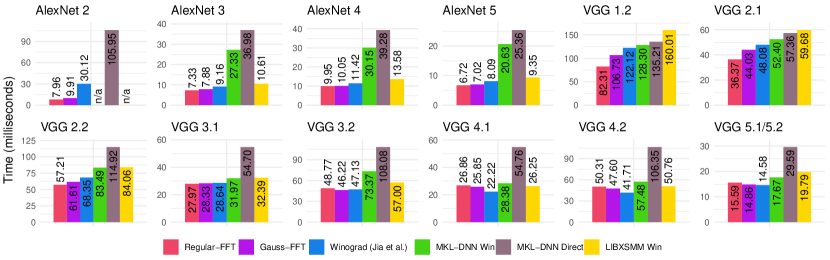
Figure 1. Convolution layers’ running time on Xeon Gold CPU.

To compare running times of the FFT and Winograd methods, we benchmarked our FFT–based implementations and the improved Winograd implementation of Jia et al. (Jia et al., 2018) by using the two most popular ConvNets, AlexNet (Krizhevsky et al., 2012) and VGG (Simonyan and Zisserman, 2014), which are frequently used for benchmarking (ima, 2018). We benchmarked the time required for the forward propagation of each distinct layers of the two networks.

Additional, publicly available, implementations were included for reference – The Winograd implementations provided by LIBXSMM (lib, 2018) and MKL-DNN (mkl, 2016), and the direct convolution provided by MKL-DNN (mkl, 2016). To the best of our knowledge, no other implementation of FFT–based methods for CPUs, beside our own, is currently available.

Both Winograd and FFT methods can work with arbitrary transform sizes. Generally, larger transform size decrease the number of required operations. However, the numerical inaccuracy of Winograd convolutions increases exponentially with transform (tile) sizes (Pan, 2016; Jia et al., 2018; Lavin and Gray, 2016). In practice, there is an upper bound on the transform size for which the Winograd produces satisfactory results. All major vendors, such as FALCON, MKL-DNN, LIBXSMM, and cuDNN (fal, 2016; lib, 2018; mkl, 2016; Appleyard, 2018) implement the Winograd algorithm with transform sizes less than or equal to $6\times 6$ . For these tile sizes, the numerical error of computation is comparable to the one that implements convolution directly.

We follow the same convention, and consider Winograd convolutions only with tile sizes of at most $6\times 6$. However, we allow the FFT methods to have an arbitrary large tile size, as they don’t suffer from such numerical instability.

Running Time Experiments

The benchmarks were performed on a total of 10 systems showed in Tbl. 1.

In Fig. 1 we show detailed results on one of the systems. Note that both LIBXSMM’s and MKL-DNN’s Winograd implementation support only kernel sizes of $3{\times}3$, and thus can not use the Winograd method for the second layer of AlexNet.

The Winograd–based method outperformed in only 3 out of 12 layers, whereas the a FFT–based method outperformed on 6 layers; and on 3 layers, they had roughly the same performances. More importantly, in the cases when the FFT methods outperformed, they did it with a larger margin, and on the layers that require more computation time. This suggests that the FFT methods can allow for significant savings in the overall computation time, when compared to the Winograd. For instance, the time spent on all convolutional layers in AlexNet using the Winograd method would consume 58.79 milliseconds, whereas the Regural–FFT method requires only 31.96 milliseconds; that is a speedup of 1.84x.

Additionally, in Fig. 2 we show the normalized running time on all other AVX512 systems (neither LIBXSMM, nor MKL-DNN support the AVX2 instruction set). The results for each individual layer are scaled based on the slowest implementation, as we are only interesting in the relative performances. Detailed results are available in Appendix. In all cases, our two FFT–based implementations as well as the modified Winograd implementation of (Jia et al., 2018) outperformed other publicly available implementations. Thus, for the rest of the paper, we will only focus on these three implementations.

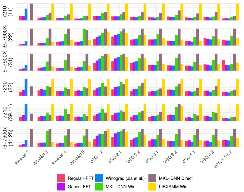
Figure 2. Normalized running time of different convolution implementations. (The systems with the same CPUs are distinguished by their CMR ).

FFT transform sizes

An important observation was that the optimal transform sizes for the FFT method were not always powers of two; they were 27 for VGG1.2, 25 for VGG2.1 and VGG2.2, 21 for VGG 3.1 and VGG3.2, 16 for VGG4.1 and VGG4.2, and 9 for VGG5.1/5.2. For AlexNet, the optimal sizes were 31 for the second layer, and 15 for all other layers. This is counter intuitive, as the common belief is that optimal FFT transforms should use sizes that only contain factors that are small primes (Frigo and Johnson, 1998; Zlateski et al., 2016b) or transforms with sizes equal to the powers of two, which is suggested by the two GPU FFT–based implementations, i.e., fbfft (Mathieu et al., 2013; Vasilache et al., 2014) and CuDNN (Chetlur et al., 2014).

Relative performances

While an FFT–method outperformed the Winograd more often than not, the relative performances varied among different layers and systems. In the rest of the paper we focus on the theoretical analysis of all the methods. We would like to understand why our findings are not aligned with the popular belief that the Winograd method should be strictly faster.

5. Performance Analysis

Our experimental observations suggested that some of the stages in both Winograd– and FFT–based approach have relatively low utilization of the system’s available FLOPS. In most, but not all, cases, these were the transform stages, which have relatively small amount of compute, but access relatively large amount of data, suggesting that their running time is bound by the memory bandwidth, and not the computational capabilities of the CPU.

For this reason, we used the Roofline (Williams et al., 2008) performance model to analyze Winograd– and FFT– based convolutions.

Roofline Performance Model

is an ISA oblivious, throughput oriented, performance model used to estimate performance of an application running on processing units, and is often used to predict performances on CPUs, GPUs, TPUs (Tensor Processing Units), etc.

It is suitable for analyzing particular methods on systems where the memory bandwidth often becomes the constraining resource. It estimates the performance bound of an algorithm as a function of its arithmetic intensity (AI), which is defined as the ratio of total floating–point operations (FPO) and the total data movement (DM) in bytes (AI= FPO/DM) between different levels of the memory hierarchy. For each level of memory hierarchy, the performance ceiling (attainable FLOPS) is determined by:

(7) $$\text{Attainable~{} FLOPS}=\min(Peak~{}FLOPS,~{}MB\times AI)$$

Where Peak FLOPS  is defined as the maximal number of floating operations per second of a given system, and MB  as system’s peak memory bandwidth. When plotted, the performance ceiling line resembles a roofline.

Here, we are interesting in the DM  between the highest level of on–chip, core–exclusive cache (typically L2 for CPUs) and off–chip, shared memory . In a systems where the L2 is shared among a small number of cores (e.g. Intel Xeon Phi series share L2 cache between two cores.), the L2 is assumed to be equally divided for exclusive usage among the cores.

DM  then accounts for all of regular and streaming stores to main memory, regular loads from main memory, and pre–fetches from main memory to either L1 or L2.

Our analysis does not consider the presence of higher level, shared caches, as on modern processors, the sizes of such caches are very limited, and can not fit the working set of a typical convolutional layers.

Additional performance ceilings for lower levels of cache, are not necessary, since in both Winograd–based and FFT–based convolutional algorithms the computation is either bounded by transfers to and from main memory, or the processor peak FLOPS, as shown in the following sections.

As the performance ceiling is set by algorithm’s arithmetic intensity (Eqn. 7), its running time can be estimated by:

(8) $$running~{}time =\frac{FPO}{\text{Attainable~{}FLOPS}}$$

$$=\frac{FPO}{\min(Peak~{}FLOPS,~{}\mathsf{MB}\times AI)}=\frac{FPO/MB}{\min(CMR,AI)}$$

$$=\begin{cases}\frac{FPO}{\mathsf{Peak~{}FLOPS}},&\mathsf{CMR}<=AI\\ \\ \frac{DM}{\mathsf{MB}},&\mathsf{CMR}>AI\end{cases}$$

Here, CMR  is the system’s compute–to–memory ratio, defined as the ratio of it’s Peak FLOPS  and MB  – the memory bandwidth. FPO  represents the total number of floating point operations required, and DM (the total amount of data movements in bytes), as defined above. The running time is compute bound when $CMR<=AI$, in which case it can be computed as $\frac{FPO}{Peak~{}FLOPS}$; otherwise, the running time is memory bound, and can be computed as $\frac{DM}{MB}$.

Estimating running time

For the Wingorad– and FFT–based convolutional layers, where the computation is composed of several sequential stages ($S$), each with a unique arithmetic intensity (AI), the running time is calculated by accumulating the running times of each stage $s\in S$:

(9) $$running~{}time_{Total}=\sum^{S}running~{}time_{s}=\sum^{S}\frac{FPO_{s}/\text{MB}}{min(\text{CMR},AI_{s})}$$

5.1. Relative Performances

We are interested in the relative performance between Winograd and FFT methods. We define $Speedup(\mathcal{A},\mathcal{B})$ as the ratio of the running times of an algorithm $\mathcal{B}$ and an algorithm $\mathcal{A}$.

(10) $$Speedup(\mathcal{A},\mathcal{B}) =\frac{running~{}time^{\mathcal{B}}_{Total}}{running~{}time^{\mathcal{A}}_{Total}}$$

A speedup greater than one indicates that the algorithm $\mathcal{A}$ is faster, and smaller than one means that the algorithm $\mathcal{B}$ is faster.

While Eqn. 9 estimates the running time of an algorithm assuming perfect utilization of the hardware, which is rarely possible in practice. However, the Eqn. 10 is also valid when the compared algorithms are equally optimized, meaning that they utilize the same percentage of the hardware capabilities.

In the Eqn. 10 the value of AI  will differ between Winograd and FFT based approaches, and will also depend on the amount of available cache size (Jia et al., 2018). Therefore, when comparing performance of two algorithms, the relative performance on a given system will depend on the CMR  ratio and the amount of available cache, but not on the absolute values of the system’s compute speed or memory throughput.

Detailed analysis on obtaining the values of AI, DM, and FPO  are presented in the Appendix A.

Using Eqn. 10 and the values of AI, DM, and FPO  calculated in the Appendix A (Tbl. 2), we estimate the speedup between the FFT–based methods and the Winograd–based one. For all three methods, the tile sizes are chosen, in a way that minimizes the total running time (Eqn. 9).

5.2. The Accuracy of the Theoretical Estimates

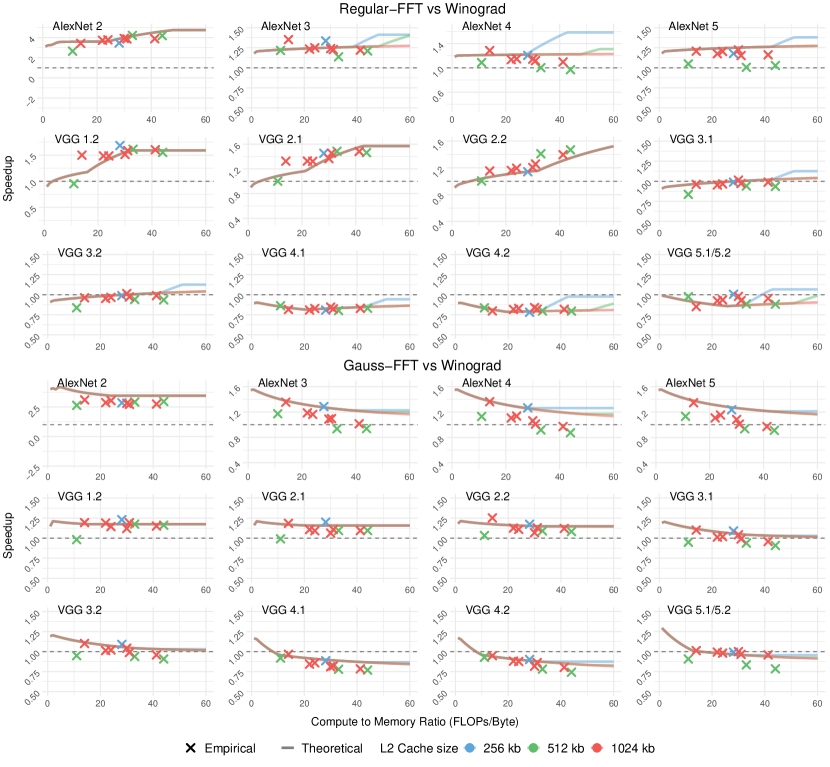
Figure 3. Theoretical estimates and empirical measurements for the speedup of Regular– and Gauss–FFT methods over the Winograd method on VGG and AlexNet. The $x$ axis represent the system’s CMR.

In Fig. 3, we plot the estimated theoretical speedup of the two FFT–based methods over the Winograd–based one. The solid lines represent the theoretical estimates of the relative performances as a function of the system’s CMR. The color of the line represents the amount of available L2 cache. The lines are drawn in a semi–translucent fashion, as they overlap in many places.

The empirical results from the benchmarks described in Section 4 are overlaid; each cross–hair represents the measurement of the relative performances on a single system. The $x$ coordinate of the cross-hairs represents the system’s compute–to–memory (CMR) ratio (see Tbl. 1), and the color represents the L2 cache sizes.

Our empirical results are consistent with our theoretical estimates. The overall relative root mean square error (rRMSE) was 0.079 for Regular–FFT vs Winograd and 0.1 for Gauss–FFT vs Winograd. The fitness  was $92.68\%$ for Regular–FFT vs Winograd and $90\%$ for Gauss–FFT vs Winograd.

5.3. Discussions

Hardware utilization

We have also measured the system utilization of each stage of the three methods. While the utilization varied across benchmarked layers and systems, on average, during the compute bound stages, 75% of theoretical peak FLOPS were attained; in memory bound stages slightly more than 85% of the theoretical memory bandwidth was achieved. This resulted in a somehow lower effective CMR, which is consistent with the results shown in Fig. 3. The empirical results are slightly shifted to the left (towards lower values of CMR), when compared to the theoretical predictions, which assume equal utilization of both the FLOPS and the memory bandwidth.

Optimality of Tile Transforms

Both “wincnn” (win, 2018) and “genfft” (Frigo and Johnson, 1998) use heuristics to minimize the number of operations for performing transforms, and might not be optimal. However, as their AIs are much smaller than the CMRs of modern systems, the computation is memory bound, and the running time of the transform stages will depend solely on the amount of data movement. The largest AI  of the FFT transforms is 5.55, and for Winograd 2.38, much lower than CMRs of the modern CPUs. The Xeon Phi Knights Landing processor has the CMR  of 11 (due to on–chip fast MCDRAM), and the Xeon Server processor family has CMRs in the range of 20–40. Hence, our theoretical analysis yield identical estimates as if the optimal number of operations were provided.

This is consistent with our experimental findings, where in some cases, tile sizes that were large primes, such as 31, were optimal. Using such sizes, the images could be divided into overlapping tiles with minimal overhead (minimal padding of the original image), which reduces both the number of required operations, and the amount of required data movements.

6. Conclusions

This paper presents experimental and analytical findings that FFT–based convolutions are, on average, faster than Winograd–based convolutions on modern CPUs.

In contrast to the popular belief that the Winograd–based method is more efficient, our experimental results of a highly optimized Winograd–based implementation and two similarly optimized FFT-based implementations on modern CPUs show that the FFT convolutions are, more often than not, faster than Wingorad ones for most commonly used ConvNet layers.

Our analysis using the Roofline model shows that whether the Winograd– or FFT–based approach is faster depends on both the layer and target hardware. However, with the tendency of increasing compute–to–memory ratio of systems with modern CPUs, the FFT–based methods tend to be faster than Winograd.

While, we primarily focused on modern multi– and many–core CPUs, which generally have larger caches, but smaller memory bandwidths than modern GPUs, we believe that our performance analysis can be applied to GPUs. Future work might include implementing and benchmarking efficient GPU–based implementations and validating performance analysis based on the Roofline model.

Appendix A Detailed Analysis

For simplicity, we assume 2D and isotropic images and kernels, as well as computation being performed with 32–bit floating point numbers (4 bytes per number). Extension to non–isotropic and $N$–dimensional images and kernels, as well as lower precision floats, is straightforward. The benchmarked implementations, described in Section 3 support an arbitrary number of dimensions, as well as non–isotropic kernels.

We follow the same notation as in Section 2, and for an arbitrary layer, use Winograd convolution $\text{F}(m^{2},r^{2})$, Regular–FFT convolution $\mathfrak{F}(m^{2},r^{2})$ and Gauss–FFT convolution $\mathfrak{G}(m^{2},r^{2})$. Here, $m$ can take an arbitrary value, whereas $r^{2}$ has to equal to the sizes of the kernels in the layer.

We proceed to present the details of all three methods and estimate the total number of operations and data movement required in each stage, from which we also calculate the arithmetic intensity of each of the three method.

A.1. Input Transform Stage

In Winograd and both FFT approaches, each of the $B\cdot C$ images ($B$ batches, each with $C$ input channels) is divided into overlapping tiles, which are then transformed. Each tile has the size of $t^{2}$ with $t=(m+r-1)$, and there is an overlap of $r-1$ pixels between adjacent tiles along both dimensions.

Each image of size $x\times x$ will thus be divided into $N=\lceil(x-r+1)/m\rceil^{2}$ tiles. If necessary, the image will be implicitly zero–padded. This yields a total of $BC\lceil(x-r+1)/m\rceil^{2}=BCN$ image tiles.

Number of required operations

Each tile ($I_{b,c,n}$) is transformed via $\tilde{I}_{b,c,n}=\mathbb{B}I_{b,c,n}\mathbb{B}^{T}$, which is a composition of two matrix–matrix multiplications. Here $I_{b,c,n}$ is the $n$–th tile of the $c$–th channel in batch $b$, and $\tilde{I}_{b,c,n}$ is its transform. Both $\mathbb{B}$ and $I_{b,c,n}$ have the size $t^{2}$, requiring a total of $4t^{3}$ operations ($2t^{3}$ per matrix–matrix multiplication). Operations are on real numbers for the Winograd approach, and on complex numbers for the FFT approaches.

The transforms can, however, be performed with much fewer operations. In the Winograd method, the matrices $\mathbb{B}$ are sparse, and contain pairs of columns with similar numbers, allowing for reuse of many intermediate results. In the FFT methods, instead of matrix multiplications, 2D real–to–complex DFT transforms are performed, which require much fewer operations ($\mu n^{2}\log n$ instead of $\mathcal{O}(n^{3})$). Here, the constant $\mu$ can vary significantly based on the size of the transform performed (Frigo and Johnson, 1998). It takes small values, when the size of the transform is a power of two, and larger values when the transform size contains large prime factors.

Instead of using a closed–form expression that gives bounds on the number of operations required, we counted the number of operations in real, optimized, implementations and stored them in a lookup tables. For Winograd, we used the Winograd matrix generator (win, 2018), as proposed in (Jia et al., 2018; Budden et al., 2016) and further reduced the number of operations using the simple optimizer provided by (Jia et al., 2018). For the FFT methods, we used the FFT codelet generator “genfft” from the FFTW library (Frigo and Johnson, 1998). We denote the number of operations required for transforming an image tile as $\text{F}^{I}(m^{2},r^{2})$ for the Winograd, $\mathfrak{F}^{I}(m^{2},r^{2})$ for Regular–FFT, and $\mathfrak{G}^{I}(m^{2},r^{2})$ for Gauss–FFT. The pre–computed lookup tables are included in our open–sourced repository.

The total number of operations required for performing all the transforms for all three methods are given in Tbl. 2.

Table 2. FLOPS, DM and AI for different stages of the Winograd ($\text{F}(m^{2},r^{2})$), Regular–FFT ($\mathfrak{F}(m^{2},r^{2})$) and Gauss–FFT ($\mathfrak{G}(m^{2},r^{2})$) methods. $N$ is the number of tiles per single image, the tiles have size of $t^{2}$ ($t=m+r-1$). The values of $c$ and $c^{\prime}$ depend on the amount of available cache, and are obtained by solving the optimization problem given in Eqn. 13.

	Stage	Winograd	Regular–FFT	Gauss–FFT
FLOPS	Input image transform	$BCN\text{F}^{I}(m^{2},r^{2})$	$BCN\mathfrak{F}^{I}(m^{2},r^{2})$	$BCN\mathfrak{G}^{I}(m^{2},r^{2})$
	Kernel transform	$CC^{\prime}\text{F}^{K}(m^{2},r^{2})$	$CC^{\prime}\mathfrak{F}^{K}(m^{2},r^{2})$	$CC^{\prime}\mathfrak{G}^{K}(m^{2},r^{2})$
	Element–wise Product	$2t^{2}BNCC^{\prime}$	$8t\lceil(t+1)/2\rceil BNCC^{\prime}$	$6t\lceil(t+1)/2\rceil BNCC^{\prime}$
	Output transform	$BC^{\prime}N\text{F}^{O}(m^{2},r^{2})$	$BC^{\prime}N\mathfrak{F}^{O}(m^{2},r^{2})$	$BC^{\prime}N\mathfrak{G}^{O}(m^{2},r^{2})$
DM	Input image transform	$4BCx^{2}+4BCNt^{2}$	$4BCx^{2}+8BCNt\lceil(t+1)/2\rceil$	$4BCx^{2}+12BCNt\lceil(t+1)/2\rceil$
	Kernel transform	$4CC^{\prime}\big{(}r^{2}+t^{2}\big{)}$	$4CC^{\prime}\big{(}r^{2}+2t\lceil(t+1)/2\rceil\big{)}$	$4CC^{\prime}\big{(}r^{2}+3t\lceil(t+1)/2\rceil\big{)}$
	Element–wise Product	$4t^{2}BN(c+\alpha c^{\prime})\dfrac{CC^{\prime}}{cc^{\prime}}$	$8t\lceil(t+1)/2\rceil BN(c+\alpha c^{\prime})\dfrac{CC^{\prime}}{cc^{\prime}}$	$12t\lceil(t+1)/2\rceil BN(c+\alpha c^{\prime})\dfrac{CC^{\prime}}{cc^{\prime}}$
	Output transform	$4BC^{\prime}N\big{(}t^{2}+m^{2}\big{)}$	$4BC^{\prime}N\big{(}2t\lceil(t+1)/2\rceil+m^{2}\big{)}$	$4BC^{\prime}N\big{(}3t\lceil(t+1)/2\rceil+m^{2}\big{)}$
AI	Input image transform	$\dfrac{N\text{F}^{I}(m^{2},r^{2})}{4x^{2}+4Nt^{2}}$	$\dfrac{N\mathfrak{F}^{I}(m^{2},r^{2})}{4x^{2}+8Nt\lceil(t+1)/2\rceil}$	$\dfrac{N\mathfrak{G}^{I}(m^{2},r^{2})}{4x^{2}+12Nt\lceil(t+1)/2\rceil}$
	Kernel transform	$\dfrac{\text{F}^{K}(m^{2},r^{2})}{4r^{2}+4t^{2}}$	$\dfrac{\mathfrak{F}^{K}(m^{2},r^{2})}{4r^{2}+8t\lceil(t+1)/2\rceil}$	$\dfrac{\mathfrak{G}^{K}(m^{2},r^{2})}{4r^{2}+12t\lceil(t+1)/2\rceil}$
	Element–wise Product	$\dfrac{cc^{\prime}}{2(c+\alpha c^{\prime})}$	$\dfrac{cc^{\prime}}{c+\alpha c^{\prime}}$	$\dfrac{cc^{\prime}}{2(c+\alpha c^{\prime})}$
	Output transform	$\dfrac{\text{F}^{O}(m^{2},r^{2})}{4t^{2}+4m^{2}}$	$\dfrac{\mathfrak{F}^{O}(m^{2},r^{2})}{8t\lceil(t+1)/2\rceil+4m^{2}}$	$\dfrac{\mathfrak{G}^{O}(m^{2},r^{2})}{12t\lceil(t+1)/2\rceil+4m^{2}}$

Data movement

The tile sizes are relatively small, much smaller than available cache; thus, once a tile is fetched from main memory, all the computation is done in–cache. Additionally, the overlapping regions between tiles need to be fetched from memory only once, as they can be stored in cache and reused for adjacent tiles.

The total data that has to be moved from main memory to cache is thus $BCx^{2}\cdot 4$ bytes – reading each of the $B\cdot C$ images of size $x^{2}$ only once. Each of the $BCN$ transformed tiles is stored back to main memory. The size for each transformed tile will depend on the method.

In Winograd convolution, transformed tiles are real tensors, and require a single 32–bit float per element, for a total of $4t^{2}$ bytes.

The FFT methods perform 2D FFT transforms of each tile. As the FFTs are performed on real tensors, the resulting transforms will be complex, conjugate–symmetric (along one of the dimensions). Only $t\lceil(t+1)/2\rceil$ complex numbers need to be stored. The Regular–FFT requires two real numbers per complex number, for a total of $8t\lceil(t+1)/2\rceil$ bytes per tile, and the Gauss–FFT requires three reals per complex number, a total of $12t\lceil(t+1)/2\rceil$ bytes per tile.

The total amount of data movement for the three methods, as well as their arithmetic intensities (AIs), is shown in Tbl. 2

A.2. Kernel Transform Stage

In all methods, each of the $C{\times}C^{\prime}$ kernels (with size $r{\times}r$) is transformed via $\tilde{W}_{cc^{\prime}}=\mathbb{G}W_{cc^{\prime}}\mathbb{G}^{T}$. The matrix $\mathbb{G}$ has size $t{\times}r$.

Computing the transform of a kernel is an equivalent procedure to performing the input transform of a zero–padded kernel, to match the size of the input tiles. In practice, the transforms are computed with implicit zero–padding. As in the input stage, we have pre–computed the number of operations required for transforming a kernel in all three methods: $\text{F}^{K}(m^{2},r^{2})$ for the Winograd, $\mathfrak{F}^{K}(m^{2},r^{2})$ for Regular–FFT. For the Gauss–FFT method, $\mathfrak{G}^{K}(m^{2},r^{2})=\mathfrak{F}^{K}(m^{2},r^{2})+2t\lceil(t+1)/2\rceil$, as we need two extra operations per complex number as described in Sec. 2.3.

All three methods need to fetch all kernel data from memory; read a total of $4CC^{\prime}r^{2}$ bytes, and store $CC^{\prime}$ transformed kernels back to main memory. The transformed kernels have size $t\times t$, and are stored in the same fashion as the transformed input tiles, requiring total of $4t^{2}$, $8t\lceil(t+1)/2\rceil$, and $12t\lceil(t+1)/2\rceil$ bytes for the Winograd, Regular–FFT and Gauss–FFT methods respectively.

The total number of operations, data movements, and AIs for transforming all kernels of a particular layer, using any of the three methods, are given in Tbl. 2.

A.3. Element–wise Products

Having all transformed input and kernel tiles, the pre–transformed output tiles $\tilde{I^{\prime}}_{b,c^{\prime},n}$ are computed via

(11) $$\tilde{I}^{\prime}_{b,c^{\prime},n} =\sum_{c=1}^{C}\tilde{I}_{b,c,n}\odot\tilde{W}_{c,c^{\prime}}$$

Here, all of the pre–transformed output tiles ($\tilde{I}^{\prime}_{b,c^{\prime},n}$), transformed input tiles $\tilde{I}_{b,c,n}$, and transformed kernels $\tilde{W}_{c,c^{\prime}}$ have the same size $t\times t$. Computing an element of the pre–transformed output tile at a location $\vec{e}$ depends only on elements of the transformed input tiles and transformed kernels at the same location, and is computed via:

(12) $$\tilde{I}^{\prime}_{b,c^{\prime},n}(\vec{e}) =\sum_{c=1}^{C}\tilde{I}(\vec{e})_{b,c,n}\cdot\tilde{W}(\vec{e})_{c,c^{\prime}}$$

Note that the equation above can be interpreted as multiplication of a matrix $U_{\vec{e}}$ of size $BN\times C$ with a matrix $V_{\vec{e}}$ of size $C\times C^{\prime}$ resulting in a matrix $X_{\vec{e}}$ of size $BN\times C^{\prime}$. For layers of modern ConvNets, values of $BN$ are much larger than $C$, which results in multiplication of tall and skinny matrices (Jia et al., 2018; Lavin and Gray, 2016). Such matrix multiplications have to be performed for each element location of $\tilde{I}^{\prime}_{b,c^{\prime},n}$.

A.3.1. Operations Required

In the Winograd method, $t^{2}$ real matrices are multiplied, requiring a total of $2t^{2}BNCC^{\prime}$ operations for the whole layer, where $N$ is the number of tiles per image.

For the FFT based methods, complex matrices are multiplied. However, only $t\lceil(t+1)/2\rceil$ locations of the pre–transformed output tiles need to be computed. As both the transformed input tiles and transformed kernels are conjugate symmetric, the pre–transformed output tiles will also be conjugate symmetric.

In the Regular–FFT method, $4$ real multiply–adds are required for performing a complex multiply–add. This gives us a total of $8t\lceil(t+1)/2\rceil BNCC^{\prime}$ FLOPs required for the whole layer. Gauss–FFT reduces complex matrix multiplications to 3 real matrix multiplications of matrices of the same size, totaling $6t\lceil(t+1)/2\rceil BNCC^{\prime}$ FLOPs required for the whole layer.

A.3.2. Data Movement

In the Winograd method, $t^{2}$ real matrix multiplications $X=U\times V$ are performed (for the rest of the section we will omit the subscript ${}_{\vec{e}}$, for clarity). In the Regular–FFT method, $t\lceil(t+1)/2\rceil$ complex matrix multiplications are performed, with the same sizes. The Gauss–FFT method replaces one complex matrix multiplication with three real matrix multiplications; thus, a total of $3t\lceil(t+1)/2\rceil$ real matrix multiplications are performed.

For modern ConvNets, the matrices $X$, $U$ and $V$ may not fit in cache, in which case standard cache–blocking approaches are employed (Gannon et al., 1988; Heinecke et al., 2015; Heinecke et al., 2016; Jia et al., 2018; Li et al., 2015), and might require some data to be moved to and/or from the main memory multiple times.

In the standard cache–blocking technique, $V$ (of size $C\times C^{\prime}$) is subdivided into equally sized matrices of size $c\times c^{\prime}$,

To minimize transfers to and from main memory, a sub–matrix of $V$ is kept in cache. A small sub–matrix of $U$, with size of $\rho{\times}c$, is fetched from memory, multiplied with the sub–matrix of $V$ stored in–cache, and accumulated to the appropriate sub–matrix of $X$. Here $\rho$ is a small number, required for efficient in–cache computation (Gannon et al., 1988; Heinecke et al., 2015; Heinecke et al., 2016; Jia et al., 2018; Li et al., 2015).

This requires transferring a total of $\rho c$ numbers from main memory, and $\rho c^{\prime}$ numbers bytes of $X$ from and then back to the main memory. A total of $\rho(c+2c^{\prime})$ numbers. In the special case, when $c=C$, only $\rho(c+c^{\prime})$ numbers need to be moved, as each sub–matrix multiplication produces the final result (no accumulation is necessary).

Total of $\nicefrac{{BNCC^{\prime}}}{{\rho cc^{\prime}}}$ such sub–matrix multiplications are performed, and require $\nicefrac{{BNCC^{\prime}}}{{cc^{\prime}}}(c+\alpha c^{\prime})$ numbers to be moved. With $\alpha$ being $1$ when $c=C$ and $2$ when $c<C$.

In the Winograd method $t^{2}$ real matrix multiplications ($X=U\times V$) are performed, thus transferring a total of $4t^{2}BN(c+\alpha c^{\prime})\nicefrac{{CC^{\prime}}}{{cc^{\prime}}}$ bytes to be moved.

In the Regular–FFT method $t\lceil(t+1)/2\rceil$ complex matrix multiplications are performed, requiring a total of $8t\lceil(t+1)/2\rceil BN(c+\alpha c^{\prime})\nicefrac{{CC^{\prime}}}{{cc^{\prime}}}$ bytes to be moved.

The Gauss–FFT replaces each of the $t\lceil(t+1)/2\rceil$ complex matrix multiplications with 3 real matrix multiplications. Total of $12t\lceil(t+1)/2\rceil BN(c+\alpha c^{\prime})\nicefrac{{CC^{\prime}}}{{cc^{\prime}}}$ bytes need to be transferred.

The total number of operations is fixed. To minimize the amount of data movements we need to choose optimal values for $c$ and $c^{\prime}$, while allowing for in–cache computation

As the values of $t$, $B$, $C$, $C^{\prime}$ and $N$ are constant, the optimal values of $c$ and $c^{\prime}$ can be chosen by solving the following optimization problem:

(13) $$\underset{\mathbf{c,c^{\prime}}}{\text{minimize}} \frac{(c+\alpha c^{\prime})}{cc^{\prime}}$$

subject to $$\mathbf{c}\mid C C \mathbf{c}$$ ( is divisible by )

$$\mathbf{c^{\prime}}\mid C^{\prime} C^{\prime} \mathbf{c^{\prime}}$$ ( is divisible by )

$$\mathbf{4\beta cc^{\prime}}\leq\frac{\text{Cache Size}}{2}$$ (fits in half cache)

Where $\alpha$ equals $1$ when $c=C$ and $2$ when $c<C$; $\beta$ is $1$ for real valued matrices, and $2$ for complex valued ones. Half the cache is allowed for sub–matrices of $V$. This is typical practice, to ensure enough space for sub–matrices of $U$ and $X$.

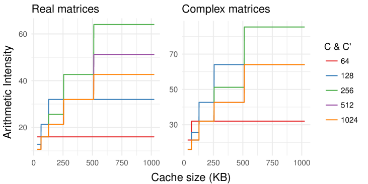
Figure 4. Arithmetic intensities for the element–wise stage given various amounts of cache. In the Winograd and Gauss–FFT method, real matrix multiplications are performed, whereas, in the Regular–FFT complex matrix multiplications are performed.

The arithmetic intensities can be then computed by dividing the number of required operations with the amount of required data movements for optimal values of $c$ and $c^{\prime}$. This results in the AIs of $cc^{\prime}/2(c+\alpha c^{\prime})$ for the Winograd and Gauss–FFT methods, and $cc^{\prime}/(c+\alpha c^{\prime})$ for the Regular–FFT method, which are equal to the AIs of real matrix, and complex matrix multiplications, respectively (Gannon et al., 1988; Heinecke et al., 2015; Heinecke et al., 2016; Jia et al., 2018).

In Fig. 4, we show the arithmetic intensities for layers with different numbers of channels as a function of cache size. The AIs of both complex (used in Regular–FFT method) and real matrix multiplication (used in Winograd and Gauss–FFT) increase with the cache size and the number of channels (C and C’). For a fixed cache size, the complex matrix multiplication allows for a higher arithmetic intensity. This indicates that the element–wise stage of the Regular–FFT method may achieve better hardware utilization than the ones of Winograd or Gauss–FFT convolution, when the cache size is a limiting resource.

A.4. Output Transform

In the output transform stage, each of the $BNC^{\prime}$ pre–transformed output tiles $\tilde{I^{\prime}}_{b,c^{\prime},n}$ is transformed from the Winograd/FFT domain back to the spatial domain via $I^{\prime}_{b,c,n}=\mathbb{A}^{T}\tilde{I}^{\prime}_{b,c,n}\mathbb{A}$. The matrix $\mathbb{A}$ has size of $t\times m$ ($t=m+r-1$), resulting in $I^{\prime}_{b,c^{\prime},n}$ having a size of $m\times m$. Here $I^{\prime}_{b,c^{\prime},n}$ is the $n$–th (non–overlapping) tile of the $c^{\prime}$-th image in batch $b$ of the final result of the convolutional layer.

Performing the inverse transforms is very similar to performing the input transforms, except that: 1) Only a subset of $m{\times}m$ elements need to be computed, and 2) Different, (inverse transform) matrices (or inverse FFT transforms) are used.

Given the analysis of the input and kernel transforms, analyzing the output transforms is straight–forward. The total number of operations, data movements, and AIs for transforming output tiles of a particular layer, using any of the three methods are given in Tbl. 2.

Appendix B Model Lookup Tables

Table 3. FLOPS required for performing Winograd transforms of a single tile or kernel.

	$r=2$			$r=3$			$r=4$			$r=5$			$r=6$			$r=7$
Method	In	Ker	Out	In	Ker	Out	In	Ker	Out	In	Ker	Out	In	Ker	Out	In	Ker	Out
$\text{F}(2^{2},r^{2})$	12	5	5	32	49	42	180	198	154	240	231	168	742	728	504	704	645	430
$\text{F}(3^{2},r^{2})$	32	24	28	180	128	128	240	170	153	742	552	460	704	518	407	-	-	-
$\text{F}(4^{2},r^{2})$	180	70	90	240	135	150	742	396	396	704	403	372	-	-	-	-	-	-
$\text{F}(5^{2},r^{2})$	240	72	99	742	260	312	704	300	325	-	-	-	-	-	-	-	-	-
$\text{F}(6^{2},r^{2})$	742	144	208	704	242	308	-	-	-	-	-	-	-	-	-	-	-	-
$\text{F}(7^{2},r^{2})$	704	130	195	-	-	-	-	-	-	-	-	-	-	-	-	-	-	-

Table 4. AIs of Winograd transforms for a single tile or kernel.

	$r=2$			$r=3$			$r=4$			$r=5$			$r=6$			$r=7$
Method	In	Ker	Out	In	Ker	Out	In	Ker	Out	In	Ker	Out	In	Ker	Out	In	Ker	Out
$\text{F}(2^{2},r^{2})$	0.17	0.10	0.10	0.25	0.49	0.53	0.90	1.21	1.33	0.83	0.95	1.05	1.89	2.14	2.38	1.38	1.43	1.58
$\text{F}(3^{2},r^{2})$	0.25	0.30	0.28	0.90	0.94	0.94	0.83	0.82	0.85	1.89	1.86	1.98	1.38	1.29	1.39	-	-	-
$\text{F}(4^{2},r^{2})$	0.90	0.60	0.55	0.83	0.75	0.72	1.89	1.52	1.52	1.38	1.13	1.16	-	-	-	-	-	-
$\text{F}(5^{2},r^{2})$	0.83	0.45	0.41	1.89	1.12	1.05	1.38	0.94	0.91	-	-	-	-	-	-	-	-	-
$\text{F}(6^{2},r^{2})$	1.89	0.68	0.61	1.38	0.83	0.77	-	-	-	-	-	-	-	-	-	-	-	-
$\text{F}(7^{2},r^{2})$	1.38	0.48	0.43	-	-	-	-	-	-	-	-	-	-	-	-	-	-	-

Table 5. FLOPS required for performing Regular–FFT transforms of a single tile or kernel.

	$r=2$			$r=3$			$r=4$			$r=5$			$r=6$			$r=7$
Method	In	Ker	Out	In	Ker	Out	In	Ker	Out	In	Ker	Out	In	Ker	Out	In	Ker	Out
$\mathfrak{F}(2^{2},r^{2})$	54	36	42	72	48	48	245	206	152	300	256	160	702	632	288	492	434	191
$\mathfrak{F}(3^{2},r^{2})$	72	28	66	245	171	186	300	192	197	702	566	444	492	380	263	1292	1088	678
$\mathfrak{F}(4^{2},r^{2})$	245	92	224	300	158	232	702	504	504	492	320	335	1292	992	758	1200	904	768
$\mathfrak{F}(5^{2},r^{2})$	300	128	274	702	325	568	492	276	400	1292	805	850	1200	792	832	2710	2118	1820
$\mathfrak{F}(6^{2},r^{2})$	702	172	636	492	206	453	1292	624	930	1200	722	912	2710	1980	1956	1416	924	1074
$\mathfrak{F}(7^{2},r^{2})$	492	146	503	1292	491	1014	1200	656	996	2710	1523	2096	1416	896	1141	3681	2583	2646
$\mathfrak{F}(8^{2},r^{2})$	1292	296	1102	1200	564	1084	2710	1108	2240	1416	823	1190	3681	2432	2808	3228	2082	2384
$\mathfrak{F}(9^{2},r^{2})$	1200	340	1176	2710	735	2388	1416	672	1262	3681	2304	3066	3228	1960	2526	3405	2254	2499
$\mathfrak{F}(10^{2},r^{2})$	2710	404	2540	1416	610	1336	3681	2052	3240	3228	1842	2672	3405	2082	2616	2904	1688	2292
$\mathfrak{F}(11^{2},r^{2})$	1416	364	1412	3681	1663	3418	3228	1504	2822	3405	1865	2897	2904	1530	2428	7793	5153	6354
$\mathfrak{F}(12^{2},r^{2})$	3681	724	3600	3228	1162	2976	3405	1628	3052	2904	1374	2562	7793	4716	6630	6068	3479	4228
$\mathfrak{F}(13^{2},r^{2})$	3228	648	3134	3405	1324	3211	2904	1246	2707	7793	4341	6892	6068	3290	4434	14418	8629	11023
$\mathfrak{F}(14^{2},r^{2})$	3405	764	3374	2904	936	2824	7793	4058	7167	6068	2660	4648	14418	8176	11410	5440	2876	4512
$\mathfrak{F}(15^{2},r^{2})$	2904	634	2976	7793	3231	7446	6068	1944	4840	14418	7305	11775	5440	2580	4682	8658	5617	6841
$\mathfrak{F}(16^{2},r^{2})$	7793	1616	7720	6068	1540	5036	14418	6668	12288	5440	2409	4878	8658	4880	7470	11852	5742	9976
$\mathfrak{F}(17^{2},r^{2})$	6068	1132	5236	14418	6266	12699	5440	2204	5078	8658	4515	7733	11852	4920	10296	26954	15562	23206
$\mathfrak{F}(18^{2},r^{2})$	14418	4516	13082	5440	1919	5282	8658	3630	8000	11852	4268	10620	26954	15072	23808	7524	3580	6622
$\mathfrak{F}(19^{2},r^{2})$	5440	1196	5490	8658	2557	8271	11852	3432	10948	26954	11815	24414	7524	3440	6837	17260	7145	12714
$\mathfrak{F}(20^{2},r^{2})$	8658	1448	8546	11852	2718	11280	26954	10880	25024	7524	3104	6988	17260	6432	13066	16128	8218	14180
$\mathfrak{F}(21^{2},r^{2})$	11852	1552	11616	26954	9981	25638	7524	2612	7213	17260	5775	13422	16128	7944	14560	21050	8309	15183
$\mathfrak{F}(22^{2},r^{2})$	26954	8396	26624	7524	2176	7363	17260	4746	13782	16128	7146	14944	21050	7586	15566	14184	6929	12426
$\mathfrak{F}(23^{2},r^{2})$	7524	1442	7570	17260	3773	14146	16128	6544	15332	21050	6308	15953	14184	6552	12760	34745	18690	31062
$\mathfrak{F}(24^{2},r^{2})$	17260	2076	14514	16128	6216	15724	21050	5100	16344	14184	6205	13098	34745	17994	31704	15480	7333	13912
$\mathfrak{F}(25^{2},r^{2})$	16128	2596	16120	21050	4118	16739	14184	5624	13440	34745	17385	32350	15480	6704	14284	38400	19470	34934
$\mathfrak{F}(26^{2},r^{2})$	21050	2516	17138	14184	4089	13786	34745	15508	33000	15480	6218	14610	38400	19142	35600	15804	7224	14352
$\mathfrak{F}(27^{2},r^{2})$	14184	2356	14136	34745	14655	33654	15480	4856	14933	38400	18275	36270	15804	6574	14669	-	-	-
$\mathfrak{F}(28^{2},r^{2})$	34745	11276	34544	15480	3842	15292	38400	17596	36944	15804	5924	14962	-	-	-	-	-	-
$\mathfrak{F}(29^{2},r^{2})$	15480	2840	15655	38400	14293	37622	15804	5302	15286	-	-	-	-	-	-	-	-	-
$\mathfrak{F}(30^{2},r^{2})$	38400	10940	38394	15804	3856	15648	-	-	-	-	-	-	-	-	-	-	-	-
$\mathfrak{F}(31^{2},r^{2})$	15804	2570	16014	-	-	-	-	-	-	-	-	-	-	-	-	-	-	-

Table 6. AIs of Regular–FFT transforms for a single tile or kernel.

	$r=2$			$r=3$			$r=4$			$r=5$			$r=6$			$r=7$
Method	In	Ker	Out	In	Ker	Out	In	Ker	Out	In	Ker	Out	In	Ker	Out	In	Ker	Out
$\mathfrak{F}(2^{2},r^{2})$	0.64	0.56	0.66	0.45	0.36	0.43	1.11	1.12	1.12	0.89	0.88	0.77	1.67	1.72	1.20	0.85	0.84	0.57
$\mathfrak{F}(3^{2},r^{2})$	0.45	0.25	0.50	1.11	1.10	1.19	0.89	0.75	0.86	1.67	1.75	1.71	0.85	0.82	0.74	1.89	1.96	1.71
$\mathfrak{F}(4^{2},r^{2})$	1.11	0.68	1.22	0.89	0.69	0.91	1.67	1.75	1.75	0.85	0.76	0.87	1.89	1.97	1.79	1.36	1.34	1.41
$\mathfrak{F}(5^{2},r^{2})$	0.89	0.62	0.94	1.67	1.25	1.75	0.85	0.72	0.95	1.89	1.75	1.85	1.36	1.27	1.43	2.68	2.93	2.90
$\mathfrak{F}(6^{2},r^{2})$	1.67	0.72	1.73	0.85	0.58	0.98	1.89	1.47	1.85	1.36	1.24	1.46	2.68	2.95	2.91	1.13	1.06	1.32
$\mathfrak{F}(7^{2},r^{2})$	0.85	0.43	0.97	1.89	1.24	1.82	1.36	1.21	1.47	2.68	2.43	2.90	1.13	1.10	1.31	2.62	2.80	2.86
$\mathfrak{F}(8^{2},r^{2})$	1.89	0.79	1.79	1.36	1.09	1.47	2.68	1.87	2.86	1.13	1.07	1.28	2.62	2.79	2.85	1.92	1.91	2.07
$\mathfrak{F}(9^{2},r^{2})$	1.36	0.69	1.46	2.68	1.30	2.80	1.13	0.91	1.27	2.62	2.78	2.91	1.92	1.88	2.07	1.83	1.95	1.95
$\mathfrak{F}(10^{2},r^{2})$	2.68	0.74	2.74	1.13	0.86	1.25	2.62	2.59	2.87	1.92	1.85	2.06	1.83	1.89	1.92	1.33	1.25	1.48
$\mathfrak{F}(11^{2},r^{2})$	1.13	0.53	1.22	2.62	2.18	2.82	1.92	1.57	2.04	1.83	1.76	2.01	1.33	1.18	1.48	3.27	3.63	3.72
$\mathfrak{F}(12^{2},r^{2})$	2.62	0.97	2.76	1.92	1.25	2.02	1.83	1.59	1.99	1.33	1.10	1.48	3.27	3.45	3.68	2.22	2.13	2.10
$\mathfrak{F}(13^{2},r^{2})$	1.92	0.71	1.99	1.83	1.33	1.96	1.33	1.02	1.48	3.27	3.28	3.63	2.22	2.08	2.10	4.86	5.03	5.02
$\mathfrak{F}(14^{2},r^{2})$	1.83	0.78	1.93	1.33	0.79	1.46	3.27	3.15	3.57	2.22	1.73	2.09	4.86	4.91	4.95	1.62	1.47	1.77
$\mathfrak{F}(15^{2},r^{2})$	1.33	0.54	1.45	3.27	2.56	3.51	2.22	1.29	2.07	4.86	4.51	4.87	1.62	1.36	1.76	2.40	2.75	2.49
$\mathfrak{F}(16^{2},r^{2})$	3.27	1.30	3.43	2.22	1.04	2.04	4.86	4.21	4.83	1.62	1.30	1.75	2.40	2.45	2.60	2.93	2.49	3.18
$\mathfrak{F}(17^{2},r^{2})$	2.22	0.78	2.02	4.86	4.03	4.75	1.62	1.21	1.74	2.40	2.32	2.57	2.93	2.18	3.15	6.23	6.47	6.90
$\mathfrak{F}(18^{2},r^{2})$	4.86	2.94	4.65	1.62	1.07	1.73	2.40	1.90	2.54	2.93	1.93	3.12	6.23	6.41	6.79	1.57	1.33	1.75
$\mathfrak{F}(19^{2},r^{2})$	1.62	0.67	1.71	2.40	1.36	2.51	2.93	1.58	3.08	6.23	5.12	6.69	1.57	1.30	1.74	3.38	2.56	3.14
$\mathfrak{F}(20^{2},r^{2})$	2.40	0.78	2.48	2.93	1.27	3.04	6.23	4.79	6.57	1.57	1.20	1.71	3.38	2.34	3.11	2.87	2.64	3.14
$\mathfrak{F}(21^{2},r^{2})$	2.93	0.73	3.00	6.23	4.45	6.45	1.57	1.02	1.69	3.38	2.14	3.08	2.87	2.60	3.11	3.54	2.58	3.17
$\mathfrak{F}(22^{2},r^{2})$	6.23	3.78	6.42	1.57	0.86	1.66	3.38	1.78	3.04	2.87	2.37	3.08	3.54	2.39	3.14	2.18	1.95	2.35
$\mathfrak{F}(23^{2},r^{2})$	1.57	0.57	1.64	3.38	1.43	3.00	2.87	2.20	3.05	3.54	2.02	3.10	2.18	1.87	2.33	5.08	5.08	5.55
$\mathfrak{F}(24^{2},r^{2})$	3.38	0.79	2.96	2.87	2.11	3.01	3.54	1.65	3.07	2.18	1.79	2.31	5.08	4.97	5.48	2.08	1.82	2.26
$\mathfrak{F}(25^{2},r^{2})$	2.87	0.89	2.98	3.54	1.35	3.03	2.18	1.64	2.29	5.08	4.86	5.41	2.08	1.68	2.25	4.92	4.68	5.40
$\mathfrak{F}(26^{2},r^{2})$	3.54	0.83	2.99	2.18	1.20	2.27	5.08	4.38	5.34	2.08	1.58	2.23	4.92	4.66	5.34	1.87	1.59	2.03
$\mathfrak{F}(27^{2},r^{2})$	2.18	0.70	2.25	5.08	4.17	5.26	2.08	1.24	2.21	4.92	4.49	5.27	1.87	1.46	2.02	-	-	-
$\mathfrak{F}(28^{2},r^{2})$	5.08	3.23	5.22	2.08	0.99	2.19	4.92	4.36	5.20	1.87	1.33	2.00	-	-	-	-	-	-
$\mathfrak{F}(29^{2},r^{2})$	2.08	0.74	2.17	4.92	3.57	5.13	1.87	1.20	1.98	-	-	-	-	-	-	-	-	-
$\mathfrak{F}(30^{2},r^{2})$	4.92	2.75	5.07	1.87	0.88	1.97	-	-	-	-	-	-	-	-	-	-	-	-
$\mathfrak{F}(31^{2},r^{2})$	1.87	0.59	1.95	-	-	-	-	-	-	-	-	-	-	-	-	-	-	-

Table 7. FLOPS required for performing Gauss–FFT transforms of a single tile or kernel.

	$r=2$			$r=3$			$r=4$			$r=5$			$r=6$			$r=7$
Method	In	Ker	Out	In	Ker	Out	In	Ker	Out	In	Ker	Out	In	Ker	Out	In	Ker	Out
$\mathfrak{G}(2^{2},r^{2})$	63	54	60	88	80	80	270	256	202	336	328	232	751	730	386	556	562	319
$\mathfrak{G}(3^{2},r^{2})$	88	60	98	270	221	236	336	264	269	751	664	542	556	508	391	1373	1250	840
$\mathfrak{G}(4^{2},r^{2})$	270	142	274	336	230	304	751	602	602	556	448	463	1373	1154	920	1300	1104	968
$\mathfrak{G}(5^{2},r^{2})$	336	200	346	751	423	666	556	404	528	1373	967	1012	1300	992	1032	2831	2360	2062
$\mathfrak{G}(6^{2},r^{2})$	751	270	734	556	334	581	1373	786	1092	1300	922	1112	2831	2222	2198	1560	1212	1362
$\mathfrak{G}(7^{2},r^{2})$	556	274	631	1373	653	1176	1300	856	1196	2831	1765	2338	1560	1184	1429	3850	2921	2984
$\mathfrak{G}(8^{2},r^{2})$	1373	458	1264	1300	764	1284	2831	1350	2482	1560	1111	1478	3850	2770	3146	3424	2474	2776
$\mathfrak{G}(9^{2},r^{2})$	1300	540	1376	2831	977	2630	1560	960	1550	3850	2642	3404	3424	2352	2918	3630	2704	2949
$\mathfrak{G}(10^{2},r^{2})$	2831	646	2782	1560	898	1624	3850	2390	3578	3424	2234	3064	3630	2532	3066	3160	2200	2804
$\mathfrak{G}(11^{2},r^{2})$	1560	652	1700	3850	2001	3756	3424	1896	3214	3630	2315	3347	3160	2042	2940	8082	5731	6932
$\mathfrak{G}(12^{2},r^{2})$	3850	1062	3938	3424	1554	3368	3630	2078	3502	3160	1886	3074	8082	5294	7208	6392	4127	4876
$\mathfrak{G}(13^{2},r^{2})$	3424	1040	3526	3630	1774	3661	3160	1758	3219	8082	4919	7470	6392	3938	5082	14779	9351	11745
$\mathfrak{G}(14^{2},r^{2})$	3630	1214	3824	3160	1448	3336	8082	4636	7745	6392	3308	5296	14779	8898	12132	5840	3676	5312
$\mathfrak{G}(15^{2},r^{2})$	3160	1146	3488	8082	3809	8024	6392	2592	5488	14779	8027	12497	5840	3380	5482	9099	6499	7723
$\mathfrak{G}(16^{2},r^{2})$	8082	2194	8298	6392	2188	5684	14779	7390	13010	5840	3209	5678	9099	5762	8352	12336	6710	10944
$\mathfrak{G}(17^{2},r^{2})$	6392	1780	5884	14779	6988	13421	5840	3004	5878	9099	5397	8615	12336	5888	11264	27483	16620	24264
$\mathfrak{G}(18^{2},r^{2})$	14779	5238	13804	5840	2719	6082	9099	4512	8882	12336	5236	11588	27483	16130	24866	8100	4732	7774
$\mathfrak{G}(19^{2},r^{2})$	5840	1996	6290	9099	3439	9153	12336	4400	11916	27483	12873	25472	8100	4592	7989	17885	8395	13964
$\mathfrak{G}(20^{2},r^{2})$	9099	2330	9428	12336	3686	12248	27483	11938	26082	8100	4256	8140	17885	7682	14316	16804	9570	15532
$\mathfrak{G}(21^{2},r^{2})$	12336	2520	12584	27483	11039	26696	8100	3764	8365	17885	7025	14672	16804	9296	15912	21779	9767	16641
$\mathfrak{G}(22^{2},r^{2})$	27483	9454	27682	8100	3328	8515	17885	5996	15032	16804	8498	16296	21779	9044	17024	14968	8497	13994
$\mathfrak{G}(23^{2},r^{2})$	8100	2594	8722	17885	5023	15396	16804	7896	16684	21779	7766	17411	14968	8120	14328	35586	20372	32744
$\mathfrak{G}(24^{2},r^{2})$	17885	3326	15764	16804	7568	17076	21779	6558	17802	14968	7773	14666	35586	19676	33386	16380	9133	15712
$\mathfrak{G}(25^{2},r^{2})$	16804	3948	17472	21779	5576	18197	14968	7192	15008	35586	19067	34032	16380	8504	16084	39361	21392	36856
$\mathfrak{G}(26^{2},r^{2})$	21779	3974	18596	14968	5657	15354	35586	17190	34682	16380	8018	16410	39361	21064	37522	16828	9272	16400
$\mathfrak{G}(27^{2},r^{2})$	14968	3924	15704	35586	16337	35336	16380	6656	16733	39361	20197	38192	16828	8622	16717	-	-	-
$\mathfrak{G}(28^{2},r^{2})$	35586	12958	36226	16380	5642	17092	39361	19518	38866	16828	7972	17010	-	-	-	-	-	-
$\mathfrak{G}(29^{2},r^{2})$	16380	4640	17455	39361	16215	39544	16828	7350	17334	-	-	-	-	-	-	-	-	-
$\mathfrak{G}(30^{2},r^{2})$	39361	12862	40316	16828	5904	17696	-	-	-	-	-	-	-	-	-	-	-	-
$\mathfrak{G}(31^{2},r^{2})$	16828	4618	18062	-	-	-	-	-	-	-	-	-	-	-	-	-	-	-

Table 8. AIs of Gauss–FFT transforms for a single tile or kernel.

	$r=2$			$r=3$			$r=4$			$r=5$			$r=6$			$r=7$
Method	In	Ker	Out	In	Ker	Out	In	Ker	Out	In	Ker	Out	In	Ker	Out	In	Ker	Out
$\mathfrak{G}(2^{2},r^{2})$	0.58	0.61	0.68	0.42	0.44	0.50	0.96	1.05	1.03	0.78	0.85	0.76	1.41	1.52	1.10	0.76	0.83	0.64
$\mathfrak{G}(3^{2},r^{2})$	0.42	0.38	0.54	0.96	1.02	1.09	0.78	0.75	0.83	1.41	1.52	1.46	0.76	0.81	0.76	1.59	1.70	1.46
$\mathfrak{G}(4^{2},r^{2})$	0.96	0.72	1.12	0.78	0.71	0.86	1.41	1.50	1.50	0.76	0.77	0.85	1.59	1.69	1.52	1.16	1.21	1.23
$\mathfrak{G}(5^{2},r^{2})$	0.78	0.66	0.89	1.41	1.14	1.53	0.76	0.74	0.91	1.59	1.51	1.58	1.16	1.15	1.26	2.22	2.39	2.31
$\mathfrak{G}(6^{2},r^{2})$	1.41	0.77	1.53	0.76	0.65	0.93	1.59	1.30	1.60	1.16	1.12	1.29	2.22	2.37	2.35	0.98	1.01	1.18
$\mathfrak{G}(7^{2},r^{2})$	0.76	0.55	0.93	1.59	1.13	1.60	1.16	1.09	1.31	2.22	1.98	2.37	0.98	1.03	1.19	2.18	2.27	2.32
$\mathfrak{G}(8^{2},r^{2})$	1.59	0.82	1.59	1.16	1.01	1.32	2.22	1.58	2.37	0.98	1.00	1.17	2.18	2.24	2.33	1.61	1.61	1.74
$\mathfrak{G}(9^{2},r^{2})$	1.16	0.73	1.32	2.22	1.18	2.36	0.98	0.90	1.16	2.18	2.22	2.40	1.61	1.58	1.75	1.55	1.65	1.67
$\mathfrak{G}(10^{2},r^{2})$	2.22	0.80	2.33	0.98	0.86	1.15	2.18	2.07	2.40	1.61	1.55	1.76	1.55	1.60	1.67	1.15	1.14	1.32
$\mathfrak{G}(11^{2},r^{2})$	0.98	0.64	1.14	2.18	1.77	2.38	1.61	1.35	1.76	1.55	1.50	1.74	1.15	1.09	1.33	2.70	2.82	2.99
$\mathfrak{G}(12^{2},r^{2})$	2.18	0.96	2.36	1.61	1.13	1.75	1.55	1.38	1.74	1.15	1.03	1.33	2.70	2.67	2.99	1.85	1.75	1.78
$\mathfrak{G}(13^{2},r^{2})$	1.61	0.76	1.75	1.55	1.20	1.73	1.15	0.98	1.34	2.70	2.54	2.97	1.85	1.71	1.79	3.97	3.78	3.97
$\mathfrak{G}(14^{2},r^{2})$	1.55	0.83	1.72	1.15	0.82	1.33	2.70	2.44	2.96	1.85	1.46	1.80	3.97	3.67	3.96	1.38	1.30	1.55
$\mathfrak{G}(15^{2},r^{2})$	1.15	0.66	1.33	2.70	2.03	2.93	1.85	1.17	1.79	3.97	3.37	3.93	1.38	1.21	1.55	2.01	2.19	2.10
$\mathfrak{G}(16^{2},r^{2})$	2.70	1.18	2.90	1.85	1.00	1.79	3.97	3.15	3.94	1.38	1.17	1.55	2.01	1.98	2.20	2.42	1.99	2.61
$\mathfrak{G}(17^{2},r^{2})$	1.85	0.82	1.77	3.97	3.02	3.91	1.38	1.11	1.55	2.01	1.88	2.19	2.42	1.78	2.60	5.06	4.74	5.43
$\mathfrak{G}(18^{2},r^{2})$	3.97	2.28	3.86	1.38	1.02	1.55	2.01	1.59	2.18	2.42	1.60	2.60	5.06	4.67	5.40	1.34	1.20	1.54
$\mathfrak{G}(19^{2},r^{2})$	1.38	0.75	1.54	2.01	1.22	2.17	2.42	1.36	2.58	5.06	3.77	5.36	1.34	1.18	1.54	2.79	2.05	2.61
$\mathfrak{G}(20^{2},r^{2})$	2.01	0.84	2.16	2.42	1.15	2.57	5.06	3.54	5.31	1.34	1.11	1.52	2.79	1.90	2.60	2.38	2.10	2.60
$\mathfrak{G}(21^{2},r^{2})$	2.42	0.79	2.55	5.06	3.30	5.26	1.34	0.99	1.52	2.79	1.76	2.59	2.38	2.06	2.59	2.92	2.06	2.64
$\mathfrak{G}(22^{2},r^{2})$	5.06	2.84	5.27	1.34	0.88	1.50	2.79	1.51	2.58	2.38	1.90	2.59	2.92	1.93	2.63	1.83	1.62	2.01
$\mathfrak{G}(23^{2},r^{2})$	1.34	0.69	1.49	2.79	1.28	2.56	2.38	1.78	2.57	2.92	1.68	2.62	1.83	1.57	2.00	4.15	3.76	4.46
$\mathfrak{G}(24^{2},r^{2})$	2.79	0.85	2.54	2.38	1.72	2.56	2.92	1.43	2.60	1.83	1.51	2.00	4.15	3.67	4.44	1.75	1.53	1.95
$\mathfrak{G}(25^{2},r^{2})$	2.38	0.90	2.54	2.92	1.22	2.59	1.83	1.41	1.99	4.15	3.58	4.41	1.75	1.44	1.95	4.02	3.48	4.36
$\mathfrak{G}(26^{2},r^{2})$	2.92	0.87	2.57	1.83	1.11	1.98	4.15	3.25	4.38	1.75	1.37	1.94	4.02	3.46	4.33	1.58	1.38	1.78
$\mathfrak{G}(27^{2},r^{2})$	1.83	0.78	1.97	4.15	3.11	4.34	1.75	1.14	1.93	4.02	3.34	4.31	1.58	1.29	1.77	-	-	-
$\mathfrak{G}(28^{2},r^{2})$	4.15	2.47	4.34	1.75	0.97	1.92	4.02	3.24	4.28	1.58	1.20	1.76	-	-	-	-	-	-
$\mathfrak{G}(29^{2},r^{2})$	1.75	0.80	1.91	4.02	2.71	4.24	1.58	1.11	1.75	-	-	-	-	-	-	-	-	-
$\mathfrak{G}(30^{2},r^{2})$	4.02	2.16	4.22	1.58	0.90	1.75	-	-	-	-	-	-	-	-	-	-	-	-
$\mathfrak{G}(31^{2},r^{2})$	1.58	0.71	1.74	-	-	-	-	-	-	-	-	-	-	-	-	-	-	-

In Tbl. 3 and Tbl. 4 we show the lookup tables used in our model to determine the number of required operations, and the arithmetic intensities for transforming a single input/output tile, or a single kernel for the Winograd method.

In Tbl. 5 and Tbl. 6 we show the lookup tables used in our model to determine the number of required operations, and the arithmetic intensities for transforming a single input/output tile, or a single kernel for the Regular–FFT method.

In Tbl. 7 and Tbl. 8 we show the lookup tables used in our model to determine the number of required operations, and the arithmetic intensities for transforming a single input/output tile, or a single kernel for the Gauss–FFT method.

Appendix C Additional Model Verification

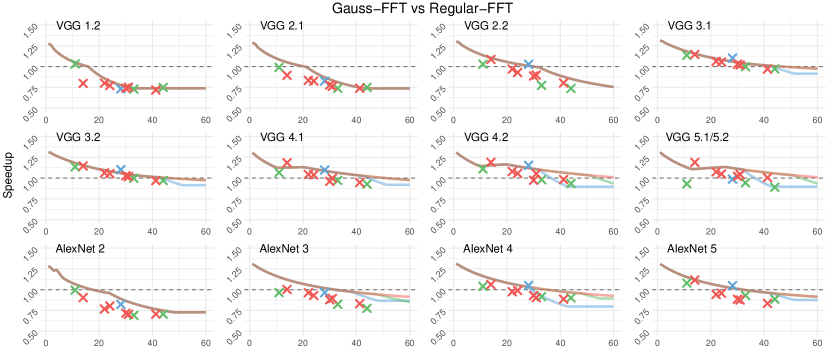
Figure 5. Theoretical estimates of our model, and empirical measurements for the speedup of the Regular– vs the Gauss–FFT method VGG and AlexNet.

In Fig. 5 we show the theoretical predictions and the empirical results of the Gauss–FFT vs the Regular–FFT methods.

Appendix D Comparing to State–of–the–art

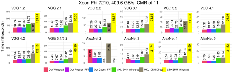
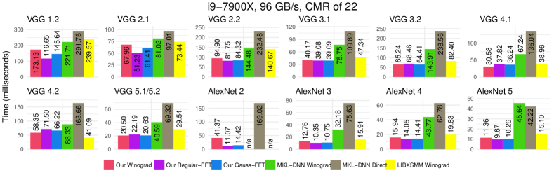
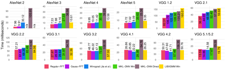
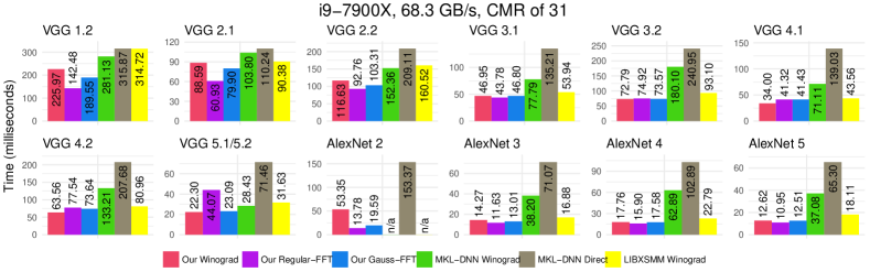
Figure 6. Running time of our implementations compared to state–of–the–art, on AVX512 capable systems.

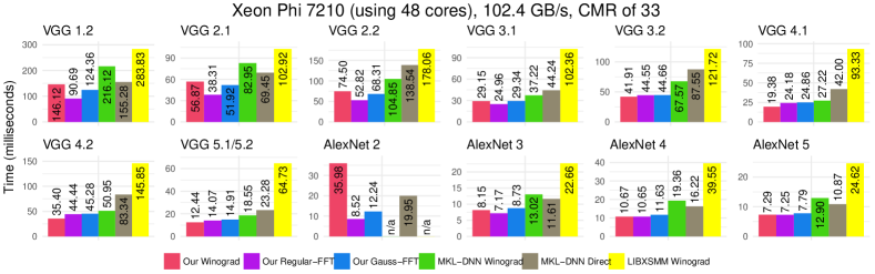
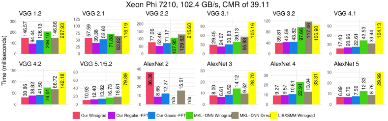
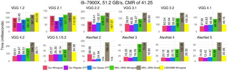
Figure 7. Running time of our implementations compared to state–of–the–art on AVX512 capable systems, continued.

In Fig. 6 and Fig. 7 we show the results of the absolute time required for processing unique layers of VGG and AlexNet of our implementation and other, state–of–the–art libraries. The benchmarks were performed on AVX512 capable systems, as the neither MKL-DNN nor LIBXSMM support AVX2.

Both MKL-DNN and LIBXSMM support only kernels of size $3\times 3$ for their Winograd implementation; thus, the measurements for the layer 2 of AlexNet, which have kerenls of size $5\times 5$ are missing.

References

- (1)
- fal (2016) 2016. FALCON Library: Fast Image Convolution in Neural Networks on Intel Architecture. "https://colfaxresearch.com/falcon-library/". (2016).
- mkl (2016) 2016. Intel(R) Math Kernel Library for Deep Neural Networks. "https://github.com/01org/mkl-dnn". (2016).
- wCo (2018) 2018. N-Dimensional Winograd–based convolution framework. https://bitbucket.org/poozh/ond-winograd. (2018).
- ima (2018) Accessed: 08-15-2018. Imagenet Winners Benchmarking. https://github.com/soumith/convnet-benchmarks. (Accessed: 08-15-2018).
- neo (2018) Accessed: 08-15-2018. Intel® Nervana reference deep learning framework. https://github.com/NervanaSystems/neon. (Accessed: 08-15-2018).
- lib (2018) Accessed: 08-15-2018. LIBXSMM. https://github.com/hfp/libxsmm. (Accessed: 08-15-2018).
- win (2018) Accessed: 08-15-2018. Wincnn. "https://github.com/andravin/wincnn". (Accessed: 08-15-2018).
- del (2018) Accessed: 08-15-2018. Winograd and FFT Convolution. https://bitbucket.org/jiazhentim/winograd-fft-conv/src/master/. (Accessed: 08-15-2018).
- Appleyard (2018) Jeremy Appleyard. Accessed: 08-15-2018. Optimizing Recurrent Neural Networks in cuDNN 5. https://devblogs.nvidia.com/parallelforall/optimizing-recurrent-neural-networks-cudnn-5/%****␣main.bbl␣Line␣125␣****. (Accessed: 08-15-2018).
- Budden et al. (2016) David Budden, Alexander Matveev, Shibani Santurkar, Shraman Ray Chaudhuri, and Nir Shavit. 2016. Deep Tensor Convolution on Multicores. arXiv preprint arXiv:1611.06565 (2016).
- Chetlur et al. (2014) Sharan Chetlur, Cliff Woolley, Philippe Vandermersch, Jonathan Cohen, John Tran, Bryan Catanzaro, and Evan Shelhamer. 2014. cudnn: Efficient primitives for deep learning. arXiv preprint arXiv:1410.0759 (2014).
- Deng et al. (2009) Jia Deng, Wei Dong, Richard Socher, Li-Jia Li, Kai Li, and Li Fei-Fei. 2009. Imagenet: A large-scale hierarchical image database. In Computer Vision and Pattern Recognition, 2009. CVPR 2009. IEEE Conference on. IEEE, 248–255.
- Frigo and Johnson (1998) Matteo Frigo and Steven G Johnson. 1998. FFTW: An adaptive software architecture for the FFT. In Acoustics, Speech and Signal Processing, 1998. Proceedings of the 1998 IEEE International Conference on, Vol. 3. IEEE, 1381–1384.
- Gannon et al. (1988) Dennis Gannon, William Jalby, and Kyle Gallivan. 1988. Strategies for Cache and Local Memory Management by Global Program Transformation. In Proceedings of the 1st International Conference on Supercomputing. Springer-Verlag, London, UK, UK, 229–254. http://dl.acm.org/citation.cfm?id=647970.761024
- Heinecke et al. (2016) Alexander Heinecke, Greg Henry, Maxwell Hutchinson, and Hans Pabst. 2016. LIBXSMM: accelerating small matrix multiplications by runtime code generation. In High Performance Computing, Networking, Storage and Analysis, SC16: International Conference for. IEEE, 981–991.
- Heinecke et al. (2015) Alexander Heinecke, Hans Pabst, and Greg Henry. 2015. Libxsmm: A high performance library for small matrix multiplications. Poster and Extended Abstract Presented at SC (2015).
- Jeffers et al. (2016) James Jeffers, James Reinders, and Avinash Sodani. 2016. Intel Xeon Phi Processor High Performance Programming: Knights Landing Edition. Morgan Kaufmann.
- Jia et al. (2018) Zhen Jia, Aleksandar Zlateski, Fredo Durand, and Kai Li. 2018. Optimizing N-Dimensional, Winograd-Based Convolution for Manycore CPUs. In Proceedings of the 23rd ACM SIGPLAN Symposium on Principles and Practice of Parallel Programming.
- Kolda and Bader (2009) Tamara G Kolda and Brett W Bader. 2009. Tensor decompositions and applications. SIAM review 51, 3 (2009), 455–500.
- Krizhevsky et al. (2012) Alex Krizhevsky, Ilya Sutskever, and Geoffrey E Hinton. 2012. Imagenet classification with deep convolutional neural networks. In Advances in neural information processing systems. 1097–1105.
- Lavin and Gray (2016) Andrew Lavin and Scott Gray. 2016. Fast algorithms for convolutional neural networks. In Proceedings of the IEEE Conference on Computer Vision and Pattern Recognition. 4013–4021.
- Li et al. (2015) Jiajia Li, Casey Battaglino, Ioakeim Perros, Jimeng Sun, and Richard Vuduc. 2015. An input-adaptive and in-place approach to dense tensor-times-matrix multiply. In Proceedings of the International Conference for High Performance Computing, Networking, Storage and Analysis. ACM, 76.
- MacLaren (1970) M Donald MacLaren. 1970. The art of computer programming. Volume 2: Seminumerical algorithms (Donald E. Knuth). SIAM Rev. 12, 2 (1970), 306–308.
- Mathieu et al. (2013) Michael Mathieu, Mikael Henaff, and Yann LeCun. 2013. Fast training of convolutional networks through ffts. arXiv preprint arXiv:1312.5851 (2013).
- Montufar et al. (2014) Guido F Montufar, Razvan Pascanu, Kyunghyun Cho, and Yoshua Bengio. 2014. On the number of linear regions of deep neural networks. In Advances in neural information processing systems. 2924–2932.
- Pan (2016) Victor Y Pan. 2016. How bad are Vandermonde matrices? SIAM J. Matrix Anal. Appl. 37, 2 (2016), 676–694.
- Rabiner and Gold (1975) Lawrence R Rabiner and Bernard Gold. 1975. Theory and application of digital signal processing. Englewood Cliffs, NJ, Prentice-Hall, Inc., 1975. 777 p. (1975).
- Simonyan and Zisserman (2014) Karen Simonyan and Andrew Zisserman. 2014. Very deep convolutional networks for large-scale image recognition. arXiv preprint arXiv:1409.1556 (2014).
- Szegedy et al. (2015) Christian Szegedy, Wei Liu, Yangqing Jia, Pierre Sermanet, Scott Reed, Dragomir Anguelov, Dumitru Erhan, Vincent Vanhoucke, and Andrew Rabinovich. 2015. Going deeper with convolutions. In Proceedings of the IEEE conference on computer vision and pattern recognition. 1–9.
- Vanhoucke et al. (2011) Vincent Vanhoucke, Andrew Senior, and Mark Z Mao. 2011. Improving the speed of neural networks on CPUs. In Proc. Deep Learning and Unsupervised Feature Learning NIPS Workshop, Vol. 1. 4.
- Vasilache et al. (2014) Nicolas Vasilache, Jeff Johnson, Michael Mathieu, Soumith Chintala, Serkan Piantino, and Yann LeCun. 2014. Fast convolutional nets with fbfft: A GPU performance evaluation. arXiv preprint arXiv:1412.7580 (2014).
- Vincent et al. (2017) Kevin Vincent, Kevin Stephano, Michael Frumkin, Boris Ginsburg, and Julien Demouth. 2017. On Improving the Numerical Stability of Winograd Convolutions. (2017).
- Williams et al. (2008) Samuel Williams, David Patterson, Leonid Oliker, John Shalf, and Katherine Yelick. 2008. The roofline model: A pedagogical tool for auto-tuning kernels on multicore architectures. In Hot Chips, Vol. 20. 24–26.
- Winograd (1980) Shmuel Winograd. 1980. Arithmetic complexity of computations. Vol. 33. Siam.
- Wulf and McKee (1995) Wm A Wulf and Sally A McKee. 1995. Hitting the memory wall: implications of the obvious. ACM SIGARCH computer architecture news 23, 1 (1995), 20–24.
- Zlateski et al. (2016a) Aleksandar Zlateski, Kisuk Lee, and H Sebastian Seung. 2016a. ZNN–A Fast and Scalable Algorithm for Training 3D Convolutional Networks on Multi-core and Many-Core Shared Memory Machines. In Parallel and Distributed Processing Symposium, 2016 IEEE International. IEEE, 801–811.
- Zlateski et al. (2016b) Aleksandar Zlateski, Kisuk Lee, and H Sebastian Seung. 2016b. ZNNi: maximizing the inference throughput of 3D convolutional networks on CPUs and GPUs. In High Performance Computing, Networking, Storage and Analysis, SC16: International Conference for. IEEE, 854–865.
- Zlateski and Seung (2017) Aleksandar Zlateski and H Sebastian Seung. 2017. Compile-time optimized and statically scheduled ND convnet primitives for multi-core and many-core (Xeon Phi) CPUs. In Proceedings of the International Conference on Supercomputing. ACM, 8.