Key words: Reaction-diffusion, localized patterns, homoclinic snaking, Belyakov-Devaney, Shilnikov analysis

1 Introduction

Localized structures are a common feature exhibited by spatially extended systems far from equilibrium. By a localized structure we mean a non-trivial pattern that is localized to some portion of the domain, with exponential decay in the far field. Such structures can be found in diverse contexts at different spatial scales ranging from biochemistry to planetary physics. Excellent reviews on localized structures can be found in [49, 1, 36].

Broadly speaking, it is possible to distinguish two types of spatially localized structures: those without and those with a distinguished spatial wavelength. The two cases are sometimes referred to respectively as isolated spikes (or pulses) and localized patterns (patches of the domain within which there is a spatially modulated periodic structure) respectively.

In this paper, we restrict our attention to the simplest setting in which one might see such localized structures: systems of two reaction-diffusion equations in one spatial dimension. Specifically, we study partial differential equation (PDE) systems of the form

(1) $$\partial_{t}U=DU_{xx}+F(U,U_{x};\lambda),$$

where $x\in[-L,L]$ with $L\gg 1$ and where the state of the system is represented by the vector unknowns $U\in\mathbb{R}^{2}$ and $\lambda\in\mathbb{R}^{p}$ is a vector of parameters. Here $D$ is a diffusion matrix and we assume that the local kinetic function $F$ is odd in components of $U_{x}$, so that the system is invariant under $x\to-x$.

Where convenient, we shall consider the limit $L\to\infty$ and study the the steady problem of (1) in the context of spatial dynamics, in which the spatial variable $x$ is considered to be a time-like co-ordinate (see e.g. [32]). In this context, the steady problem to (1) may be considered to be a four-dimensional reversible system in the phase space variables $(U,U_{x})$ and a localized structure corresponds to an orbit $U_{h}(x)$ that is homoclinic to the homogeneous equilibrium solution $U_{0}$ as $x\to\pm\infty$. One can then use the theory of homoclinic orbits in reversible system, see e.g. [28, 56, 19, 8], which shows that such localized solutions are persistent under parameter variation. Very different kinds of behavior can be observed however, depending on the nature of the spatial eigenvalues of the problem linearized about $U_{0}$. Broadly speaking, real eigenvalues correspond to isolated spike-like solutions whereas complex eigenvalues lead to the possibility of localized patterns. See Figure 1 which illustrates the qualitative differences between these two cases.

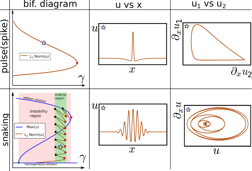
Figure 1: Qualitative differences between pulse solutions (top half) and localized patterns (bottom half). In the leftmost column, a sketch of the bifurcation diagram of each solution is represented in which the vector $L_{2}$-norm is plot against a scalar parameter $\gamma$. The middle column depicts one representative component of a particular solution (distinguished with a star on the left), as a graph against $x$. The rightmost column shows a planar projection of the solution in phase space. [Numerical results used here are from: (pulses(spike)) the generalized cell polarity model (3) below with parameter values (4) using $\delta$ as a continuation parameter when $\gamma=14$; (sanking) using the Swift-Hohenberg equataion $\partial_{t}u=-(1+\partial_{x}^{2})^{2}u-\mu u+\nu u^{2}-u^{3}$ on a finite domain with $\nu=1.6$ and $\mu$ as the continuation parameter.]

1.1 Isolated spikes

Spike-like isolated or single-pulse states correspond to homoclinic steady solutions of the system (1) in which the decay to the far field is eventually monotonic and their representation in the spatial phase space is rather simple (see the upper panels of Figure. 1). Stable versions of such pulses often arise via a single fold bifurcation from an unstable pulse that bifurcates at small amplitude from a homogeneous equilibrium (see the bifurcation diagram sketched in the top-left panel of Figure 1).

Such solutions can be observed in a wide variety of models. Two important examples are Gray-Scott or Schnackenberg-like reaction-diffusion systems — which can be analyzed using either geometric singular perturbation theory (as, for example, in the works of Doelman et al. [30, 31]) or using matched asymptotic expansions (as in the work of Ward et al. [35, 50]) — and the parametrically driven non-linear Schrödinger equation (see, for example, the works of Barashenkov et al. [6, 7] and references therein). In some contexts such localized states are called dissipative solitons (see e.g. [2, 49]) and methods exist to approximate their dynamics on large domains via point-like approximations (see e.g. [45]). In two or more spatial dimensions such solutions can behave like particles and can weakly interact with each other. Although some mechanisms exist (such as so-called inclination or orbit-flips, see e.g. [4, 47] and references therein) for creating stable multi-peaked versions, in general such localized states do not form infinite families of bound states, owing to their lack of oscillatory tails. Also, unlike solitons of integrable systems, dissipative solutions can gain permanent oscillatory dynamics, for instance through Hopf bifurcations, which can give rise to quasi-periodic or fully chaotic behaviors.

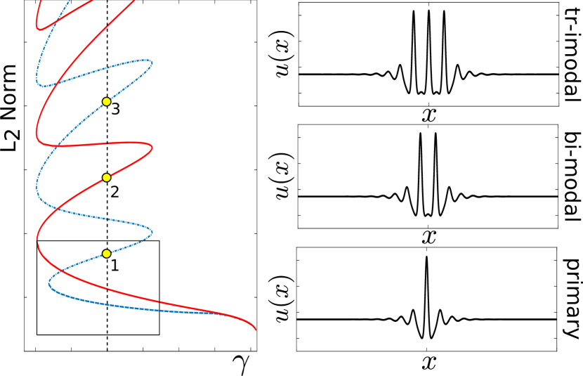
Figure 2: More details of the homoclinic snake in Figure. 1, showing two inter-twined branches; the continuous and dashed lines represent branches of symmetric solutions with even and odd number of large peaks, respectively (without considering the oscillating tails). The square in the bottom of left panel, is the area where the primary (single peaked) orbit exists. One component of the solution profile at each numerical label is depicted in the corresponding graph to the right. For both curves in the main graph, the localized solutions are stable along portions of the graph that have positive slope and lose stability at the fold points.

1.2 Localized patterns and homoclinic snaking

A localized pattern represents a qualitatively different type of stationary solution state to (1). In contrast to spikes, such states possess a spatial wave-length and feature decaying oscillatory tails as the solution tends to the far field. These solutions typically occur as part of an infinite family of solutions, members of which can be characterized by their number of maxima outside of the tail regions (see the lower panels in Figure 1 and also Figure 2).

One way to describe such localized patterns is to think of them as the interaction of two fronts, where at least one of the steady states that the fronts are connecting posses a spatial wave-length [23]. In this situation, it is sometimes possible to use a weakly non-linear analysis to estimate the bifurcation diagram of localized patterns (e.g. [54]), which typically resembles the one illustrated in the bottom-left panel of Figure 1. This technique assumes a large distance between the fronts.

An alternative way of understanding localized patterns via spatial dynamics assumes instead that the localized patterns are not weakly interacting, but arise from the unfolding a heteroclinic connection between a saddle-focus equilibrium and a saddle-like periodic orbit. The period of the periodic orbit provides the internal wavelength of the patters. As a consequence of the reversibility, the unfolding of the heteroclinic connections creates a countable infinite number of homoclinic orbits, which correspond to the localized patterns. The simplest examples among these infinite families are typically connected in a bifurcation diagram like the one depicted in Figure. 2 which has been dubbed a homoclinic snake [56].

There is now a rich literature on the homoclinic snaking scenario. For example, as explained in the context of Swift-Hohenberg-like equations in the work of Burke & Knobloch [16, 17]. Kozyreff & Chapman [38, 22] among others (e.g. [26]), have explained how the snake arises from beyond-all-orders perturbations of a degenerate (super-to-subcritical transitioning) pattern formation instability of the homogeneous steady state. In addition, Beck et al [8] have provided rigorous justification of what can happen away from this singular limit (see also [43] for more cases). In particular, it is important to draw a distinction between cases where there is and where there is not variational structure (a conserved Hamiltonian-like quantity of the spatial dynamics), whether or not there is additional symmetry and also between finite and infinite domains; e.g. [24, 14, 15, 34, 25, 37].

There are also analogues of homoclinic snaking in higher spatial dimensions, where localized versions of rolls, hexagonal lattices and target patterns can be observed [40, 5]. The snaking diagrams are more complex, and not all details are known, but see [44, 39, 11] for the state of the art. For the preset paper, though, we shall exclusively concern models of the form (1) in one spatial dimension.

1.3 Outline

This paper has been motivated by a number of recent studies in which both localized patterns and isolated spikes have been observed in different parts of parameter space of reaction-diffusion systems of the form (1). One motivation for our study is the work of Zelnik et al [57] on an ecological model, in which exactly the same transition we study in this paper is observed, although a theoretical explanation of the spike to localized pattern transition was lacking. Similar transitions have been observed in our recent work on a simple model for cellular polarity formation [55] and in a continuum model for urban crime [41]. These two models will be revisited in detail in Section 2.

The rest of the paper is organized as follows. Through the two examples discussed in section 2, a hypothesis is formed that the transition from localized patterns to isolated spikes is driven by where the first fold of the homoclinic snake passes through the curve in a parameter plane where there is a transition from complex to real spatial eigenvalues, through a double real eigenvalue. We dub such a codimension-two bifurcation a non-transverse Belyakov-Devaney bifurcation. Section 3 contains the main results of the paper, a partial unfolding of such a non-transverse Belyakov-Devaney bifurcation, using a Shilnikov-style approach — an adaptation to the analysis in [18] to the particular codimension-two problem in question. Section 4 than makes asymptotic predictions from the analysis on the nature of the bifurcation and compares these to results for the two examples. The paper ends with a careful discussion in Section 5, indicating exactly what has and has not been shown, and pointing to directions of future work.

2 Snake to spike transition in two examples

We have chosen two example systems of the form (1) to illustrate the phenomenon we seek to explain. As we shall see, these models have very different nonlinear terms and arise in quite distinct contexts, which serves to illustrate the ubiquity of the transition we seek to understand (see also Section 5 for discussion of further examples).

The steady problem of (1) can be re write as a four-dimensional, reversible system of ordinary differential equations

(2) $$\frac{dy}{dx}=f(x,\lambda),\;\;y\in\mathbb{R}^{4}=(u,u_{x},v,v_{x}).$$

As first shown by Devaney [27, 28] (see also the reviews [19, 20]), the multiplicity of homoclinic orbits to a symmetric equilibrium $y_{0}$ in such a systems depends crucially on the eigenvalues of the linearization around $y_{0}$. Reversibility ensures eigenvalues come in symmetric pairs $\pm\lambda$. If the equilibrium is hyperbolic (all eigenvalues have non-zero real parts) then a generic homoclinic orbit will be isolated and should persist under parameter perturbation. If the eigenvalues are complex $\lambda=\pm\rho\pm i\omega$, then each homoclinic orbit should be accompanied by an infinite multiplicity of families of $N$-pulse homoclinic orbits. For each $N$, the family is characterized by a string a $N-1$ integers $(i_{1},,i_{2},\ldots i_{N-1})$, where each $i_{k}\in\mathbb{Z}^{+}$ represents the distance between each pulse in terms via the number of half-oscillations close to $y_{0}$. There can be restrictions on which strings are admissible, that is which ones correspond to true multi-pulse orbits. For example, without a conserved first integral then only palindromic strings, which correspond to symmetric orbits, will lead to persistent multi-pulse orbits; see [33, 18] for details.

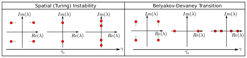
Figure 3: Eigenvalues of the linearization around a homogeneous solution of system (2) in the vicinity of a Turing instability (left panel) and Belyakov-Devaney transition (right panel). The arrow at the bottom shows the parameter $\gamma$ crossing a critical value $\gamma_{c}$.

Homoclinic snaking, as in Figure. 2, typically occurs when a primary homoclinic orbit emerges sub-critically from a point of double imaginary eigenvalues $\pm i\omega$. Such a codimension-one bifurcation is sometimes called a Hamiltonian-Hopf bifurcation, or reversible 1:1 resonance point, and is equivalent to the fundamental pattern formation instability of the underlying PDE, which, as the domain size tends to infinity, corresponds to the accumulation point of infinitely Turing bifurcations [12]. With slight abuse of notation, we shall refer to such a double-imaginary eigenvalue bifurcations in the spatial dynamics (cf. left panel of Figure 3) as a Turing bifurcation. Note that the localized patterned states that arise from the fold bifurcations within the homoclinic snake are typically quite distinct from the multi-pulse homoclinic orbits, because their large peaks are not close to the primary homoclinic orbit, but to a finite amplitude periodic orbit; and the separations between the peaks is governed by the period of the periodic orbit, not by the linearization at the equilibrium. Nevertheless each localized pattern arising in the snake will give rise to infinitely many further multi-pulse orbits just like the primary orbit does.

The central theme of this paper is how homoclinic snaking can break up, as a second parameter is modified; specifically what happens when the pinning region extends to cover the whole of a parameter region in which the spatial eigenvalues are complex. The boundary case of interest is when these eigenvalues become a double real pair, see the right panel of Figure 3. The case of primary homoclinic orbit passing through such a transition was dubbed in [19] a Belyakov-Devaney bifurcation because of the similarity to the codimension-two bifurcation in non-reversible systems first described by Belyakov [9]; see also [10] for these ideas applied in the context of reversible systems. Here, the infinite family of multi-pulse orbits disappear via the distance between each pulse tending to infinity as the critical eigenvalue transition is approached. Where convenient, in what follows we shall sometimes abuse notation and describe the eigenvalue transition of four complex eigenvalues to four real eigenvalues through a double-real-eigenvalue transition as being a Belyakov-Devaney transition, irrespective of whether the equilibrium has a homoclinic orbit connecting to it or not. What we shall find though is that as the folds of the homoclinic snake approach a Belyakov-Devaney transition, then the distinction between a multipulse homoclinic orbit and a localized pattern becomes blurred as the period of the periodic orbit at the center of the pattern tends to infinity and the pattern itself becomes part of the family of multi-pulse orbits associated with the primary homoclinic orbit.

Notice that is often possible to find analytical expressions for the Turing and Belyakov-Devaney transitions, because they are properties of the linearized system (see examples below). However, in order to study the existence and bifurcations of homoclinic orbits away from special distinguished points, the use of numerical methods is required. Throughout this paper, we shall use AUTO [29] with Neumann boundary conditions on a half-interval $[-L,0]$ or $[0,L]$ for a sufficiently large $L$ that the solution in the far field is very close to the homogeneous equilibrium. Using this approach, we will only capture homoclinic orbits that are symmetric under the reversibility. Also, this paper shall only consider existence and multiplicity of homoclinic solutions, the stability and PDE dynamics associated with such localized solutions shall not be of specific concern.

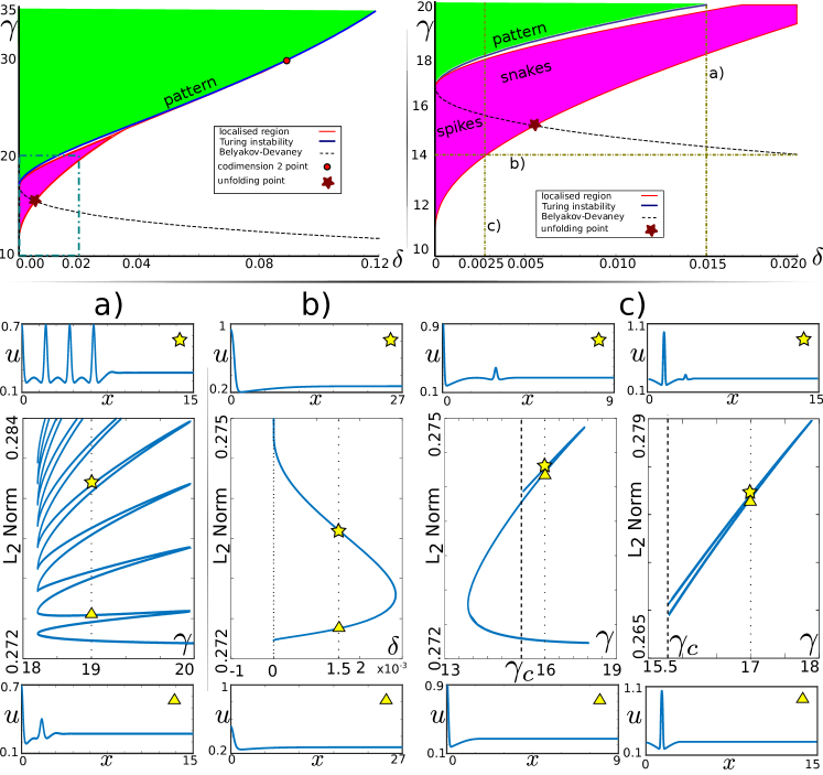
Figure 4: Top panel: Two-parameter bifurcation diagram of the general cell polarity model (3) with other parameters as in (4). The right-hand panel is a zoom of the area within the dot-dashed box in the left-hand panel. The solid (blue) line corresponds to the Turing bifurcation which is sub-critical to the left of the red circle and super-critical to the right. The dashed line corresponds to the Belyakov-Devaney transition. The thin red lines delineating the pink shaded region correspond to where localized patterns or spikes are observed. The codimension-two point of concern in this paper is represented by the maroon star at the intersection of the Belyakov-Devaney line and the right-hand edge of the localized pattern region. Alphabetically labeled dot-dashed lines in the right-hand panel correspond to one-parameter continuations depicted in the Bottom panels, insets to which show solution profiles depicted on the half-interval $x\in[0,L]$ for $L\gg 1$; see text for details.

2.1 A Generalized Cell Polarity Model

The first example is the model, arising in cell biology, that was previously studied by the present authors in [55]. This is a generalization, through the addition of source and loss terms, of the simple canonical model for the spatial patterning of G-proteins underlying cellular polarity formation proposed by Mori, Jilkine & Edelstein-Keshet [46]. It can be written in the form

(3a) $$\partial_{t}u =\delta\partial_{xx}u+[F(u,v)-\varepsilon\theta u],$$

(3b) $$\partial_{t}v =\partial_{xx}v-[F(u,v)-\varepsilon\alpha],\qquad x\in\left[-L,L\right],\quad\partial_{x}(u,v)(\pm L)=0,$$

(3c) where $$\quad F(u,v)=\gamma\frac{u^{2}v}{1+u^{2}}-\eta u+v.\qquad$$

Here $u(x,t)$ and $v(x,t)$ represent the concentrations of active and inactive species respectively of a structural $G$-protein, and $\delta\ll 1$ is the ratio of their diffusion rates. The function $F(u,v)$ represents the local kinetics of the activation step parameterized by $\mathcal{O}(1)$ parameters $\eta$, $\gamma$. The specific form of $F$ is not important, provided that it exhibits bistability. We fix all the parameters except two, the diffusion ratio $\delta$ and the parameter which controls the non-linearity in the model $\gamma$. Following [55], we choose

(4) $$\varepsilon=1,\quad\eta=5.2,\quad\theta=5.5,\quad\alpha=1.5.$$

The unique homogeneous equilibrium of (3) is given by

(5) $$(u_{0},v_{0})=\left(\frac{\alpha}{\theta},\frac{\alpha(\varepsilon\theta+\eta)(\theta^{2}+\alpha^{2})}{\theta[\theta^{2}+\alpha^{2}(1+\gamma)]}\right):=\left(\frac{\alpha}{\theta},\beta_{0}+\varepsilon\beta_{1}\right).$$

Performing a linear stability analysis around this equilibrium, the condition for the linear transitions in question are [55]:

(6) $$\varepsilon\theta\partial_{v}F-\frac{(\partial_{u}F-\delta\partial_{v}F-\varepsilon\theta)^{2}}{4\delta}=0,\qquad\mbox{with }k_{c}^{2}=\frac{\partial_{u}F-\delta\partial_{v}F-\varepsilon\theta}{2\delta},$$

with critical wavenumber $k_{c}^{2}>0$ corresponding to the Turing instability and $k_{c}^{2}<0$ to a Belyakov-Devaney transition. The double pairs of spatial eigenvalues at the Turing bifurcation are $\pm i\omega$ where $\omega=k_{c}$, and $\pm\lambda=\mp k_{c}$ at the Belyakov-Devaney transition.

The organization of simplest patterned states of model (3) in the $(\delta,\gamma)$-plane is summarized in Figure 4 (full details are given in [55]). The top panel depicts the single curve (6) for the case $k_{c}^{2}>0$ and $k_{c}^{2}<0$ using a continuous blue line and a dashed black line respectively. The red dot represents the point where the Turing bifurcation changes from supercitical (for larger $\delta$) to subcritical. From this point emerges a pinning region, shaded pink, in which localized solutions occur. A maroon star marks the codimension two point where the Belyakov-Devaney transition and the first fold of the primary homoclinic orbit (right-hand boundary of the localized pattern region) occur simultaneously. This point, which we term the unfolding point, will be the subject of our study in Section 3.

The lower panels of Figure 4 depict various cross-sections through the bifurcation diagram of the simplest, primary homoclinic orbit, with a yellow triangle and star used to depict two specific homoclinic solutions plot on the half-interval $x>0$ Panel (a) shows a regular homoclinic snake, for a case where $\gamma$ remains entirely in the parameter region corresponding to complex eigenvalues. There are infinitely many folds in theory but the simulation is always carried out on a finite domain.

In contrast, panel (b) shows a case where localized patterns are contained exclusively in the real eigenvalue part of parameter space. In [55], the only stable localized solution observed in this parameter region is the larger-amplitude single spike solution observed on the upper portion of this branch. Note that both the small and large amplitude pulse survive all the way to the singular limit $\delta\to 0$, with the latter disappearing at zero amplitude deviation from the homogeneous equilibrium.

Panel (c) of Figure 4 shows a hybrid case where the primary localized solution crosses the Belyakov-Devaney transition, at $\gamma=\gamma_{c}$, indicated by a vertical dashed line. The figure is divided into two separate portions for the primary orbit and the two-pulse orbits that were formerly part of the homoclinic snake. Note how the first fold of the primary orbit has passed through $\gamma_{c}$. After the second fold, which creates a three-peaked orbit, the primary branch turns around and then terminates at $\gamma_{c}$. The mechanism of termination is that the solution becomes delocalized; the outer two pulses disappear towards $x=\pm\infty$ as $\gamma\to\gamma_{c}$. We find that all other branches of the snake, including the intertwined branch with an even number of pulses never cross $\gamma_{c}$, but are split into separate pieces with solutions becoming delocalized as they approach $\gamma_{c}$. The second portion of panel (c) shows the continuation of the two-pulse orbit which exists only for $\gamma>\gamma_{c}$. Note how both the primary and the two-pulse homoclinic orbit gain an extra small maximum after returning from their right-most fold, which also becomes delocalized as $\gamma\to\gamma_{c}$.

2.2 An urban Crime-Wave model

In 2008 Short et al [53] derived a system of PDEs for crime density within an urban area, based on mean-field approximation to a stochastic agent-based model. The model was able to replicate the behaviors observed in real crime data, in particular that crime seems to be concentrated in localized areas (hot-spots). Subsequently, Lloyd and O’Farrell [41] studied the same model in both one and two spatial dimensions in an attempt to understand the origin of such localization. Here we just focus on the one-dimensional model, which can be written in the form

(7a) $$\partial_{t}A =\eta^{2}\partial_{xx}A-A+\beta+\rho A,$$

(7b) $$\partial_{t}\rho =\partial_{xx}\rho-2\frac{\rho}{A}\partial_{xx}A-2\frac{\partial_{x}\rho\partial_{x}A}{A}+2\frac{\rho(\partial_{x}A)^{2}}{A^{2}}-\rho A+\mu-\beta.$$

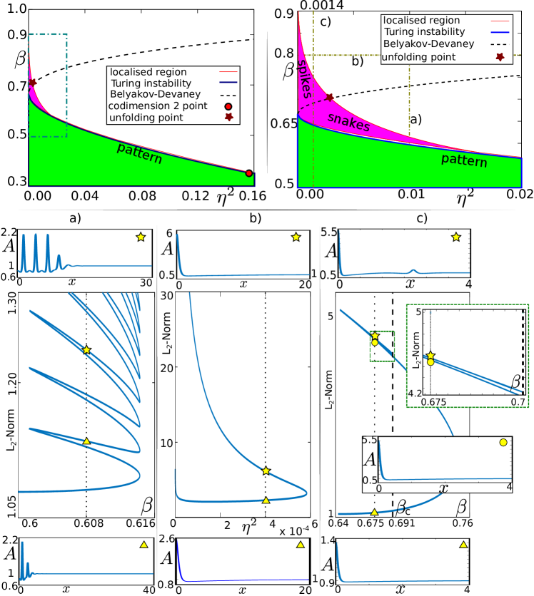
Figure 5: Top panel: Two-parameter bifurcation diagram for the urban crime model (7) for $\mu=1$, using the same conventions as in Figure. 4. Bottom panel: One-parameter bifurcation diagrams along paths a)–c)

Here $A$ represent the attractiveness of an area to burglars and $\rho$ the density of criminals. This system possesses three dimensionless parameters, $\beta$, $\mu$ and $\eta^{2}$, which, for the sake of clear distinction between parameters and state variables, we have renamed from the notation used in [41]. System (7) has a homogeneous equilibrium given by

$$\left(\begin{array}[]{c}A_{h}\\ \rho_{h}\end{array}\right)=\left(\begin{array}[]{c}\mu\\ 1-\frac{\beta}{\mu}\end{array}\right).$$

Performing a linear stability analysis around this equilibrium [41] one finds that a Turing instability occurs whenever

(8) $$\beta=\frac{2}{3}\mu-\eta^{2}\frac{\mu^{2}}{3}-\frac{2}{3}\mu\sqrt{\mu\eta^{2}},\quad\text{with}\quad k_{c}^{2}=\sqrt{\frac{\mu}{\eta^{2}}},$$

and a Belyakov-Devaney transition when

(9) $$\beta=\frac{2}{3}\mu-\eta^{2}\frac{\mu^{2}}{3}+\frac{2}{3}\mu\sqrt{\mu\eta^{2}}.$$

Figure 5 presents a two-parameter bifurcation diagram, using the same conventions and colors as the last example. The bifurcation diagram was essentially already present [41] (See Figure. 1(e) of that paper), but the transition between spikes and localized patterns illustrated the bottom panel of Figure 5 was not analyzed. Note how, qualitatively speaking, the scenario observed here is identical to that in the previous example.

3 Unfolding the non-transverse Belyakov-Devaney transition

The examples studied suggest that the transition we describe is generic, to that end we now construct a plausible analysis, to predict what happens in a neighborhood of the key codimension-two bifurcation in question. That is, we provide a partial unfolding of the case of a fold in a primary homoclinic orbit first touching the Belyakov-Devaney transition and see if this can explain the phenomenon observed. We shall use the paradigm of spatial dynamics, in the limit $L\to\infty$, in which we consider the steady problem and the spatial variable $x$ is replaced by a time-like variable $t$ in what follows (which should not be confused with the actual temporal variable of the time-dependent PDEs).

We use the method pioneered by L.P. Shil’nikov, see [52] and references therein, specifically an adaptation to the previous work of the second author [18], that considered symmetric homoclinic orbits to an equilibrium with complex eigenvalues in a reversible system. Here, we will consider a perturbation of the the primary homoclinic orbit, which will provide the conditions for the existence of 2-pulse homoclinic orbits. The spirit of the analysis is that of a formal, justified calculation; we shall not attempt to provide rigorous statements.

3.1 Generic hypotheses

We are interested in a description of homoclinic orbits in a neighborhood of the codimension-two point where a primary homoclinic orbit of a four-dimensional reversible system undergoes a fold at a Belyakov-Devaney point. This point has been distinguished in the two-parameter bifurcation diagrams of Figures 4 and 5 with a maroon star and termed the unfolding point. In the spirit of [18], we consider the four-dimensional dynamical system given by the differential equations

(10) $$\frac{dy}{dt}=f(y;\varepsilon,\nu)\quad\varepsilon,\nu\in\mathbb{R},\quad y\in\mathbb{R}^{4},\quad f\in C^{r},\quad(r\geq 2).$$

We shall make a number of generic hypotheses

H1

We suppose that the system is reversible, that is, there is a linear operator $\mathcal{R}$ which satisfies

$$\mathcal{R}\circ\mathcal{R}=I\quad\text{and}\quad\mathcal{R}\cdot f=-f\circ\mathcal{R}.$$

It will be useful for our analysis to define the two-dimensional symmetric section $S=\mbox{Fix}(\mathcal{R})$. Whenever an orbit intersects $S$, then we can reverse time without loss of generality so that the orbit is symmetric, that is

(11) $$\mathcal{R}y(t)=y(-t).$$

To apply the present analysis to systems of two-reaction diffusion equations, as in Section 2.1, we have in mind that $y=(u,u_{x},v,v_{x})^{T}$ and that $\mathcal{R}$ acts to reverse the derivative variables

$$\mathcal{R}(u,u_{x},v,v_{x})^{T}=(u,-u_{x},v,-v_{x})^{T}\>,$$

and similarly for the crime wave model.

H2

We suppose that the system (10) has an isolated hyperbolic stationary point which lies within $\mathcal{S}$; for the sake of simplicity we take this stationary point to be the origin $y=0\in S$. We suppose that the linearisation at the stationary point is hyperbolic and has two-dimensional stable and unstable eigenspaces. Then, by standard theorems on reversible systems (see e.g. [28, 19, 51]), the two-dimensional stable and unstable manifolds $W^{s,u}(0)$)

$$W^{s}(0)=\{y\in\mathbb{R}^{4}|\lim_{t\to\infty}\phi_{t}(y)=0\}\quad\text{and}\quad W^{u}(0)=\{y\in\mathbb{R}^{4}|\lim_{t\to-\infty}\phi_{t}(y)=0\}$$

(where $\phi_{t}$ is the flow corresponding to the differential equation) are symmetric images of each other, $\mathcal{R}W^{u}(0)=W^{s}(0)$.

H3

We shall make the additional technical assumption that a smooth co-ordinate change has been undertaken that flattens the stable and unstable manifolds within a small neighborhood $B$ of the origin. Moreover, we assume that within $B$ the dynamics is completely linear.

Note that the above hypothesis may be rigorously justified using $C^{1}$ conjugacy results for reversible systems, see for example [51]. We omit the precise details here, because our purpose is to achieve a plausible argument for an asymptotic scaling, rather than a rigorous result. We make a further assumption about the linearisation at the origin

H4

We suppose that at the parameter value $\varepsilon=0$ the eigenvalues of the linearized system within $B$ are degenerate and form two non-semisimple pairs of double real eigenvalues $\pm\rho$, for some $\rho>0$. Moreover we suppose that $\varepsilon$ is a generic unfolding parameter that is designed in such a way that the characteristic polynomial of $Df(0;\varepsilon,\nu)$ can be written

(12) $$P(\lambda)=[(\lambda-\rho)^{2}-\varepsilon][(\lambda+\rho)^{2}-\varepsilon]\>.$$

Hence for $\varepsilon<0$ the equilibrium is a saddle focus with eigenvalues

$$\lambda=\pm\rho\pm i\sqrt{-\varepsilon}\>+\mathcal{O}(\varepsilon),$$

whereas for $\varepsilon>0$ there the origin is a real saddle with eigenvalues

$$\lambda=\pm\rho\pm\sqrt{\varepsilon}\>+\mathcal{O}(\varepsilon),$$

see Figure 6 for corresponding phase portraits.

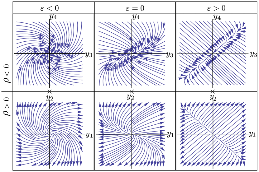
Figure 6: Phase portraits of the linear dynamics within the stable and unstable eigenspaces a neighborhood $B$ of the origin, as described in using the local co-ordinates in Sec. 3.2. In each column, the upper and lower panels correspond to stable and unstable manifolds, respectively. Chosen parameter values are $\rho=1$ and from left to right $\varepsilon=-0.8$, $0$ and $0.8$.

Next, we make assumptions about the existence of a degenerate homoclinic orbit.

H5

We suppose that at the codimension-two point $\varepsilon=\nu=0$ Are we also assuming that $\rho\ll\varepsilon$) there exists a symmetric homoclinic orbit $y=\gamma(t)$ that is not wholly contained within $B$, and is such that

$$\gamma(0)\in S\quad\text{and}\quad\lim_{t\to\pm\infty}\gamma(t)=0.$$

Moreover, we suppose that $B$ is chosen to be sufficiently close to the origin that the trajectory $\gamma(t)$ contains only one connected component that is outside of $B$. Thus we shall refer to $\gamma$ as being the primary homoclinic orbit. We also suppose that $B$ is chosen such that the additional non-degeneracy condition (17) is satisfied. The particular degeneracy of the primary orbit we assume when $\nu=\varepsilon=0$ is that there is a quadratic tangency between $W^{u}(0)$ and $S$ at $\gamma(0)$. We suppose that the parameter $\nu$ unfolds this tangency in a generic way such that, for all sufficiently small $|\varepsilon|$, there are two transverse intersections between $W^{u}(0)$ and $S$ near $\gamma(0)$ for small $\nu<0$, and no nearby intersection for small $\nu>0$ (see Figure  7 (b)).

H6

We assume certain non-degeneracy conditions concerning the general position of $W^{u}$ and $S$ at $\nu=0$, as set out in equations (31) and (32) in Section 3.3 below.

Our goal in what follows is to describe the fate of multi-pulse homoclinic orbits in a neighborhood of $\gamma$ for small unfolding parameters $\varepsilon$ and $\nu$ (assuming all other parameters remain fixed). To do this we use the well-established technique of approximation of the dynamics through appropriate Poincaré maps (see Figure 7).

3.2 Local map near the origin

We shall now set up local co-ordinates within $B$. Given H1-H3 it is possible to choose a local system of coordinates $y=(y_{1},y_{2},y_{3},y_{4})^{T}$, such that he linear system can be written

(13) $$\dot{y}=\mathbb{J}y\quad\text{where}\quad\mathbb{J}=\left(\begin{array}[]{cc}A_{+}&0\\ 0&A_{-}\end{array}\right),\quad\text{and}\quad A_{\pm}=\left(\begin{array}[]{cc}\pm\rho&1\\ \varepsilon&\pm\rho\end{array}\right).$$

In this coordinate system, the dynamics in the local stable and unstable manifolds $W^{s}_{\rm loc}(0)$ and $W^{u}_{\rm loc}(0)$ correspond to the uncoupled subsystems associated with matrices $A_{-}$ and $A_{+}$, respectively, as illustrated in Figure 6. Under this construction, note that $y_{2}$ (and $y_{4}$) are in the direction of the unstable (stable) eigenvector when $\varepsilon=0$, and $y_{1}$ (and $y_{3}$) are in the direction of the generalized eigenvector. Moreover, without loss of generality we suppose that within the local co-ordinate system, reversibility acts so that

$$\mathcal{R}(y_{1},y_{2},y_{3},y_{4})^{T}\to(y_{3},y_{4},y_{1},y_{2}).$$

Furthermore, we choose the box $B$ to take the form

(14) $$B=\{y\in\mathbb{R}^{4}|y_{1}^{2}+y_{2}^{2}\leq h^{2},\mbox{ and }y_{3}^{2}+y_{4}^{2}\leq h^{2}\},\qquad\mbox{for some $h\ll 1$}.$$

It is also useful to define polar coordinates within $B$

(15) $$y=\left(\begin{array}[]{c}y_{1}\\ y_{2}\\ y_{3}\\ y_{4}\end{array}\right)=\left(\begin{array}[]{c}r_{+}\cos\theta_{+}\\ r_{+}\sin\theta_{+}\\ r_{-}\cos\theta_{-}\\ r_{-}\sin\theta_{-}\end{array}\right),\quad\text{with }0\leq r_{\pm}<h\text{ and }0\leq\theta_{\pm}<2\pi.$$

We can now define local Poincaré sections on $\partial B$. In particular we define incoming and outgoing sections

incoming: $$\quad\Pi_{-}=\{y=(r_{+},\theta_{+},r_{-},\theta_{-})\in B\;|\;r_{-}=h\},$$

outgoing: $$\quad\Pi_{+}=\{y=(r_{+},\theta_{+}r_{-},\theta_{-})\in\mathbb{R}^{4}\;|\;r_{+}=h\}.$$

It is straightforward to show that these sections are transverse to the flow, provided $|\varepsilon|$ is sufficiently small. Another useful Poincaré section inside $B$ is the ’halfway through’ section, containing a local piece of $S$, given by

(16) $$\mbox{halfway :}\quad\Pi_{\rm sym}=\{y=(r_{+},\theta_{+},r_{-},\theta_{-})\in B\;|\;r_{+}=r_{-}\}.$$

Note that, topologically, each of $\Pi_{{\rm sym},+,-}$ represents a solid torus, see Figure 7 (b) and (c) for an illustration.

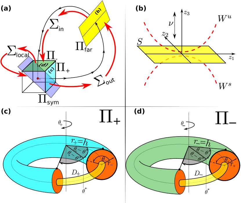
Figure 7: Overview of the construction of the Poincaré maps in the vicinity of the codimension-two homoclinic orbit being analyzed, illustrating the geometry in each of the Poincaré sections $\Pi_{+}$, $\Pi_{-}$, $\Pi_{\rm sym}$ and $\Pi_{\rm far}$; see text for details. (a) The primary homoclinic orbit is represented by a continuous black line, and the stationary point at the origin by a red dot. The action of the Poincaré maps $\Sigma_{\rm out}$, $\Sigma_{\rm in}$, and $\Sigma_{\rm local}$ is indicated by bold red arrows. Note the true dynamics are in $\mathbb{R}^{4}$, although the overall sketch is a 3D projection. Panels (b)-(d) indicate the three-dimensional geometry within each of the Poincaré sections $\Pi_{\rm far}$, $\Pi_{+}$ and $\Pi_{-}$, respectively. In each case the local co-ordinate system is illustrated.

Hypotheses (H5) and (H6) guarantee the existence of an isolated homoclinic orbit $\gamma(t)$ when $\nu=\eta=0$. This orbit intersects $\Pi_{+}$ at a single point

$$\gamma_{+}=\gamma\cap\Pi_{+}:\quad(r_{+},\theta_{+},r_{-},\theta_{-})=(h,\theta_{*},0,0),$$

for some $\theta_{*}\in[0,2\pi)$. We shall assume the non-degeneracy hypothesis

(17) $$\theta_{*}\neq 0$$

By reversibility it intersects $\Pi_{-}$ at

$$\gamma_{-}=\gamma\cap\Pi_{-}:\quad(r_{+},\theta_{+},r_{-},\theta_{-})=(0,0,\theta_{*},h).$$

We shall now define $D_{\pm}$ to be small neighborhoods of $\gamma_{\pm}$ in $\Pi_{\pm}$ (see panels (b) and (c) in Figure 7):

$$D_{-}=\{y\in\Pi_{-}\;|\;|\theta_{-}-\theta_{*}|\leq h,\;r_{+}\leq h^{2}\},$$

$$D_{+}=\{y\in\Pi_{+}\;|\;|\theta_{+}-\theta_{*}|\leq h,\;r_{-}\leq h^{2}\}.$$

In terms of polar co-ordinates, the linear equations can be written

(18) $$\dot{r}_{\pm} =r_{\pm}((1+\varepsilon)\sin\theta_{\pm}\cos\theta_{\pm}\pm\rho),$$

(19) $$\dot{\theta}_{\pm} =\varepsilon\cos^{2}\theta_{\pm}-\sin^{2}\theta_{\pm}.$$

We can obtain analytical solutions to the initial-value problem for (18),(19). Note that the equations in the stable and unstable subspaces are completely decoupled and can be solved independently. For definiteness we shall consider the dynamics in the unstable subspace; the stable case can be obtained by simply replacing $\rho$ by $-\rho$ in what follows. The equation for $\theta_{+}$ can be solved through separation of variables, to obtain

(20) $$\tan(\theta_{+}(t))=\sqrt{\varepsilon}\tanh(\sqrt{\varepsilon}(t+C_{\theta_{+}}(\sqrt{\varepsilon})),\quad C_{\theta_{+}}(\sqrt{\varepsilon})=\frac{\operatorname{arctanh}}{\sqrt{\varepsilon}}\left(\frac{\tan(\theta_{+}(0))}{\sqrt{\varepsilon}}\right),$$

where $C_{\theta_{+}}$ is the constant of integration, to be can determined from the initial condition $\theta_{+}(0)=\theta_{+0}$ . Substituting (20) into the $r_{+}$-equation, we can again solve using separation of variables. The complete solution in terms of the initial conditions $\left.(r_{+},\theta_{+})\right|_{t=0}=(r_{+0},\theta_{+0})$ can be written as

(21) $$\tan\theta_{+}(t) =\frac{\varepsilon\tanh(\sqrt{\varepsilon}t)+\sqrt{\varepsilon}\tan\theta_{+0}}{\sqrt{\varepsilon}+\tanh(\sqrt{\varepsilon}t)\tan\theta_{+0}}$$

(22) $$r_{+}(t) =\sqrt{\frac{\Theta(t,\theta_{+0};\varepsilon)}{\Theta(0,\theta_{+0};\varepsilon)}}r_{+0}e^{\rho t},$$

where

$$\Theta(t;C_{\theta};\varepsilon)=(1+\varepsilon)\cosh(2\sqrt{\varepsilon}(t+C_{\theta}))+1-\varepsilon;$$

that is,

(23) $$\Theta(t,\theta_{+,0};\varepsilon)= \frac{(1+\varepsilon)(\cosh(2\sqrt{\varepsilon}t)(\varepsilon+\tan^{2}\theta_{+,0})+2\sqrt{\varepsilon}\sinh(2\sqrt{\varepsilon}t)\tan\theta_{+0})}{(\varepsilon-\tan^{2}\theta_{+0})}+(1-\varepsilon).$$

It will be useful to consider the limit $\varepsilon\to 0$ in the expressions (21) and (22). Using l’Hôpital’s rule, the components of the solution are

(24) $$\lim_{\varepsilon\to 0}\theta_{+}(t)=\arctan\left(\frac{\tan\theta_{+0}}{1+t\tan\theta_{+0}}\right),$$

(25) $$\lim_{\varepsilon\to 0}r_{+}(t)=r_{+0}e^{\rho t}\sqrt{(t\sin\theta_{+0}+\cos\theta_{+0})^{2}+\sin^{2}\theta_{+0}}.$$

Using these definitions, we can build a local map

$$\Sigma_{\rm local}:\>D_{-}\subset\Pi_{-}\to\Pi_{\rm sym}.$$

by following the local flow through the box $B$ until a trajectory strikes $\Pi_{\rm sym}$; see Figure 7(a).

In terms of polar coordinates (15), we have

$$\Sigma_{\rm local}:\>\left(\begin{array}[]{c}r_{+}^{(1)}\\ \theta_{+}^{(1)}\\ h\\ \theta_{-}^{(1)}\end{array}\right)\to\left(\begin{array}[]{c}r^{(2)}\\ \theta_{+}^{(2)}\\ r_{-}^{(2)}\\ \theta_{-}^{(2)}\end{array}\right),\qquad\mbox{where}\quad r_{+}^{(2)}=r_{-}^{(2)}.$$

Using (22), we find

(26) $$r_{+}^{(2)}=r_{+}^{(1)}\sqrt{\frac{\Theta(\tau,\theta_{+}^{(1)},\varepsilon)}{\Theta(0,\theta_{+}^{(1)},\varepsilon)}}e^{\rho\tau},\qquad r_{-}^{(2)}=h\sqrt{\frac{\Theta(\tau,\theta_{-}^{(1)},\varepsilon)}{\Theta(0,\theta_{-}^{(1)},\varepsilon)}}e^{-\rho\tau},$$

where $\Theta$ is given by (23) and $\tau$ is the time of flight from $\Pi_{-}$ to $\Pi_{s}$, which as yet unknown. The condition to be in $\Pi_{s}$ is enforced by equating the two expressions in (26). Thus, we obtain

(27) $$\left(\frac{r_{+}^{(1)}}{h}\right)^{2}\frac{\Theta(\tau,\theta_{+}^{(1)},\varepsilon)\Theta(0,\theta_{-}^{(1)},\varepsilon)}{\Theta(\tau,\theta_{-}^{(1)},\varepsilon)\Theta(0,\theta_{+}^{(1)},\varepsilon)}=e^{-4\tau\rho},\qquad 0<r_{+}^{(1)}<h\>.$$

Equation (27) is a transcendental equation for $\tau$ in terms of the initial conditions $r^{(1)}_{+}$, $\theta^{(1)}_{+}$ and $\theta^{(1)}_{-}$ in $\Pi_{-}$; in general, it does not have a closed-form solution. Nevertheless, note that $\tau=0$ when $r_{+}^{(1)}=h$. Conversely, when $r_{+}^{(1)}\to 0$, which corresponds to approaching a solution in the stable manifold (which by construction never leaves $B$), the expression (27) reduces to $e^{-4\tau\rho}=0$, implying $\tau\to\infty$ as expected. Note further, by definition of $D_{-}$, $r_{+}^{(1)}/h\ll 1$. This restriction implies that we are interested in cases where $\tau\gg 1$. We are also interested in the role of $\varepsilon$ as an unfolding parameter, therefore it makes sense to consider the expression (27) asymptotically for large $\tau$ and in the limit limit $\varepsilon\to 0$. Using (25), we find in the limit $\varepsilon\to 0$, that

$$\left(\frac{r_{+}^{(1)}}{h}\right)^{2}\left(\frac{\sin^{2}\theta_{+}^{(1)}\tau^{2}+2\sin\theta_{+}^{(1)}\cos\theta_{+}^{(1)}\tau+1}{\sin^{2}\theta_{-}^{(1)}\tau^{2}+2\sin\theta_{-}^{(1)}\cos\theta_{-}^{(1)}\tau+1}\right)=e^{-4\tau\rho}.$$

Now, for $\tau\gg 1$, the rational function on the left-hand side can be approximated by its leading-order terms, from which we obtain

$$\left|\frac{r_{+}^{(1)}}{h}\right|\left|\frac{\sin\theta_{+}^{(1)}}{\sin\theta_{-}^{(1)}}+\mathcal{O}(\tau^{-1})\right|=e^{-2\tau\rho}.$$

Using this equation, an approximate expression for $\tau$ when $\varepsilon$ and $r_{+}^{(1)}$ are small is

(28) $$\tau=\frac{\log}{2\rho}\left(\left|\frac{h\sin\theta_{-}^{(1)}}{r_{+}^{(1)}\sin\theta_{+}^{(1)}}+\mathcal{O}\left(\frac{1}{r_{+}^{(1)}}\right)\right|\right)+\mathcal{O}(\varepsilon),$$

which is valid for $\theta_{-}^{(1)}\neq n\pi\neq\theta_{+}^{(1)}$ for any $n\in\mathbb{Z}$. This condition can be guaranteed by redefinition of the origin of the angular co-ordinates if necessary.

Finally, substituting the expression (28) for $\tau$ into the equations (22) and (21), we find an explicit expression for the map $\Sigma_{\rm local}$ in the limit of small $r_{+}^{(1)}$ and $\varepsilon$.

Using similar techniques, it is straightforward to use the estimates (22) and (25) to define the map that takes initial condition in $D_{-}$ all the way through $B$ to $\Pi_{+}$ using similar techniques. Such a construction is not necessary for the present analysis where we only seek to study two-pulse orbits. But we would need that map if we wanted to obtain a description of the complete dynamics near $\gamma$ or to construct three-pulse or higher order multi-pulse orbits (see [18] in the non-degenerate case).

3.3 Global Maps

Next we will define maps $\Sigma_{\rm out}$ (and $\Sigma_{\rm in}$) that respectively flow in forward and backward time from a neighborhood $D_{+}$ ($D_{-}$) along $\gamma(t)$ into a neighborhood of $\gamma(0)$. Note that it is possible to construct such maps so that they are images of each other under the reversibility $\mathcal{R}$. In order to make such a construction, we need to define a suitable local Poincaré section, $\Pi_{\rm far}$, say, transverse to the flow at $\gamma(0)$; see Figure 7 (a). In order to build the maps, we need to define local coordinates $(z_{1},z_{2},z_{3})$ within $\Pi_{\rm far}$ as depicted in Figure 7 (b).

Note we are free to make this choice by defining $z_{1}$ to be the co-ordinate direction that points along the direction of the tangency between $W^{u}$ and $S$. Then we suppose that $z_{2}$ is the orthogonal direction to this within $S$ and $z_{3}$ is the direction orthogonal to $S$ within $\Pi_{\rm far}$. Under these assumptions, the reversibility acts according to

(29) $$\mathcal{R}\left(\begin{array}[]{c}z_{1}\\ z_{2}\\ z_{3}\end{array}\right)=\left(\begin{array}[]{c}z_{1}\\ z_{2}\\ -z_{3}\end{array}\right).$$

Now, the map $\Sigma_{\rm out}$ maps $D_{+}\subset\Pi_{+}\to\Pi_{\rm far}$, our starting point $y^{(1)}$ lies in $D_{+}$. Considering this limit in (15), we find the initial point to be

$$y^{(1)}=\left(\begin{array}[]{c}y_{1}\\ y_{2}\\ y_{3}\\ y_{4}\end{array}\right)=\left(\begin{array}[]{c}h\cos(\theta^{*}+s)\\ h\sin(\theta^{*}+s)\\ r_{-}^{(1)}\cos\theta_{-}^{(1)}\\ r_{-}^{(1)}\sin\theta_{-}^{(1)}\end{array}\right),$$

where $s\in[-h,h]$ is a small parameter that parametrises the piece of $W^{u}_{\rm loc}$ in $D_{+}$, such that $s=0$ at the point $\gamma_{+}$. Consequently we can reduce the coordinates to $(s,y_{3},y_{4})\in\Pi_{+}$ and the map can be simplified to

$$\Sigma_{\rm out}:\left(\begin{array}[]{c}s\\ y_{3}\\ y_{4}\end{array}\right)\longmapsto\left(\begin{array}[]{c}z_{1}\\ z_{2}\\ z_{3}\end{array}\right).$$

The map $\Sigma_{\rm out}$ maps $y^{(1)}$ into a point in $\Pi_{\rm far}$, $s$ is a co-ordinate that parametrises a tangent vector to trajectories in the unstable manifold at $\gamma_{+}$, and is transverse to $\gamma(t)$. We expect such a vector to be mapped into a direction tangential to the unstable manifold in $\Sigma_{\rm far}$ transverse to the primary homoclinic orbit. Additionally, the hypothesis H5 requires that this piece of $W^{u}\cap\Sigma_{\rm far}$ to be quadratically tangent to $S$ when $\nu=0$ (see Figure 7(b)). Notice too that the map should be a diffeomorphism and hence invertible. Under these assumptions, and assuming no further degeneracy, $\Sigma_{\rm out}$ can be written as

(30) $$\begin{pmatrix}z_{1}\\ z_{2}\\ z_{3}\end{pmatrix}=\begin{pmatrix}as,\\ \eta_{23}y_{3}+\eta_{24}y_{4}\\ \eta_{33}y_{3}+\eta_{34}y_{4}+bs^{2}+\nu\end{pmatrix}+\mathcal{O}(y^{2}),$$

for arbitrary real constants $a$, $b$ and $\eta_{i,j}$, satisfying some mild hypotheses as described below. The parameter $\nu$ controls how the stable and unstable manifolds intersect with $S$ as specified in H5 and depicted in Figure 7(b). That is, for $\nu>0$ the manifolds do not intersect there are is no primary homoclinic orbit; whereas, for $\nu<0$, there are two transverse intersections. The sense of the tangency and the choice of co-ordinates implies that must assume that

$$a>0,\qquad b>0.$$

The second global map, can be defined by exploiting the reversibility:

$$\Sigma_{\rm in}=\mathcal{R}(\Sigma_{\rm out})^{-1}\circ\mathcal{R},$$

see Figure 7. The map $\Sigma_{\rm out}^{-1}:\Pi_{\rm far}\to\Pi_{+}$ is given by

$$\Sigma_{\rm out}^{-1}\left(\begin{array}[]{c}z_{1}\\ z_{2}\\ z_{3}\end{array}\right)=\left(\begin{array}[]{c}y_{2}\\ y_{3}\\ y_{4}\end{array}\right),\quad\text{where}\quad s=\frac{z_{1}}{a},\quad y_{3}=\frac{\left|\begin{array}[]{cc}z_{2}&\eta_{24}\\ \xi&\eta_{34}\end{array}\right|}{\psi},\quad y_{4}=\frac{\left|\begin{array}[]{cc}\eta_{23}&z_{2}\\ \eta_{33}&\xi\end{array}\right|}{\psi},$$

and $\xi=z_{3}-\nu-b\left(\frac{z_{1}}{a}\right)^{2}$. Notice that in order to be invertible we require,

(31) $$\psi:=\left|\begin{array}[]{cc}\eta_{23}&\eta_{24}\\ \eta_{33}&\eta_{34}\end{array}\right|\neq 0.$$

In what follows, we shall also require further non-degeneracy assumptions; namely that

(32) $$\eta_{24}\neq 0\qquad\mbox{and}\quad 0\neq\eta_{23}\neq-\eta_{24}\tan(\theta^{*}).$$

Using the defined maps, we can establish the conditions for multi-pulse orbits. We shall restrict attention to two-pulse orbits. In principle, $n$-pulse orbits for any $n$ can be constructed similarly.

3.4 Constructing two-pulse orbits

We start by considering a point $y_{0}$ near the primary orbit within $W^{u}$ in $D_{+}$ to subsequently find a set of conditions for the image of $y_{0}$ under the map

$$\Sigma_{\rm total}:D_{+}\longmapsto\Pi_{\rm sym}$$

to lie in the intersection of the symmetric section with $\Pi_{\rm sym}$. By construction, such a point represents a homoclinic orbit that passes a neighborhood of $\gamma(0)$ twice; a two-pulse orbit.

The map $\Sigma_{\rm total}$ can be defined as

(33) $$\Sigma_{\rm total}=\Sigma_{\rm local}\circ\mathcal{R}\circ\Sigma_{\rm out}^{-1}\circ\mathcal{R}\circ\Sigma_{\rm out}:D_{+}\longmapsto\Pi_{\rm sym}.$$

We consider the initial point $y_{0}$ in a line segment of length $2s\ll h$, around the primary homoclinic solution $\gamma$ within intersection of $D_{+}\cap W^{u}(0)$. That is, we take

$$r_{-}=0,\quad r_{+}=h,\quad\theta_{+}=\theta^{*}+s,\quad|s|\ll 1,$$

and consequently

(34) $$y_{0}=\left(\begin{array}[]{c}y_{1}\\ y_{2}\\ y_{3}\\ y_{4}\end{array}\right)=\left(\begin{array}[]{c}h\cos(\theta^{*}+s)\\ h\sin(\theta^{*}+s)\\ 0\\ 0\end{array}\right).$$

We proceed to compose each successive Poincaré map in (33). The image of $y_{0}$ under the $\Sigma_{\rm out}$ is

$$\Sigma_{\rm out}\left(\begin{array}[]{c}s\\ 0\\ 0\end{array}\right)\longmapsto\left(\begin{array}[]{c}as\\ 0\\ bs^{2}+\nu\end{array}\right).$$

Applying the reversing transformation (29), we obtain

$$\mathcal{R}\circ\Sigma_{\rm out}\left(\begin{array}[]{c}s\\ 0\\ 0\end{array}\right)\longmapsto\left(\begin{array}[]{c}as\\ 0\\ -bs^{2}-\nu\end{array}\right),$$

and after applying $\Sigma_{\rm out}^{-1}$, we obtain

$$\Sigma_{\rm out}^{-1}\circ\mathcal{R}\circ\Sigma_{\rm out}\left(\begin{array}[]{c}s\\ 0\\ 0\end{array}\right)=\left(\begin{array}[]{c}s\\ 2\frac{\eta_{24}}{\psi}(\nu+bs^{2})\\ -2\frac{\eta_{23}}{\psi}(\nu+bs^{2})\end{array}\right):=\left(\begin{array}[]{c}\zeta_{2}\\ \zeta_{3}\\ \zeta_{4}\end{array}\right)\in\Pi_{+}\>.$$

We have to apply $\mathcal{R}$ again to reach $\Pi_{-}$. Within $B$ and its boundary, the reversing transformation acts to exchange the roles of $\{y_{1},y_{2}\}$ and $\{y_{3},y_{4}\}$, and so we obtain

$$y_{3} =h=r_{-}\cos\theta_{-}=r_{-}\cos(\theta*+\zeta_{2})=r_{-}\cos(\theta^{*}+s)$$

$$y_{4} =r_{-}\sin\theta_{-}=r_{-}\sin(\theta*+\zeta_{2})=r_{-}\sin(\theta^{*}+s)$$

$$y_{1} =\zeta_{3}=\frac{2\eta_{24}}{\psi}(\nu+bs^{2})=r_{+}\cos\theta_{+},$$

$$y_{2} =\zeta_{4}=\frac{-2\eta_{23}}{\psi}(\nu+bs^{2})=r_{+}\sin\theta_{+}.$$

After rearrangement, we find

(35) $$r_{-} =h,$$

$$\theta_{-} =\theta^{*}+s,$$

(36) $$r_{+} =\frac{2(|\nu+bs^{2}|)}{|\psi|}\sqrt{\eta_{24}^{2}+\eta_{23}^{2}},$$

$$\tan\theta_{+} =-\frac{\eta_{23}}{\eta_{24}}=-\eta,$$

$$\sin\theta_{+} =\frac{-\eta_{23}}{\sqrt{\eta_{23}^{2}+\eta_{24}^{2}}}\quad\text{which implies}\quad r_{+}\sin\theta_{+}=-2\eta_{23}\left|\frac{\nu+bs^{2}}{\psi}\right|=-\frac{1}{\varphi}|\nu+bs^{2}|,$$

where $\eta$ and $\varphi$ have been defined to simplify the subsequent algebra. Note that $\varphi$ is well defined and non-zero by the nondegeneracy assumption (32)

We finally need to apply the map

$$\Sigma_{\rm local}:\left(\begin{array}[]{c}r_{+}^{(1)}\cos\theta_{+}^{(1)}\\ r_{+}^{(1)}\sin\theta_{+}^{(1)}\\ r_{-}^{(1)}\cos\theta_{-}^{(1)}\\ r_{-}^{(1)}\sin\theta_{-}^{(1)}\end{array}\right)\longmapsto\left(\begin{array}[]{c}r_{+}^{(2)}\cos\theta_{+}^{(2)}\\ r_{+}^{(2)}\sin\theta_{+}^{(2)}\\ r_{-}^{(2)}\cos\theta_{-}^{(2)}\\ r_{-}^{(2)}\sin\theta_{-}^{(2)}\end{array}\right),$$

and impose that the image is in the symmetric section. This is the condition for the existence of two-pulse orbits. In terms of our coordinates, we need that

(37) $$r_{+}^{(2)}=r_{-}^{(2)}\quad\text{and}\quad\theta_{+}^{(2)}=\theta_{-}^{(2)}.$$

The first condition is automatically met by the definition of the Poincaré section $\Pi_{s}$ (16) and also by definition of the time of flight $\tau$. Hence, it is sufficient to impose the second condition to establish the existence of the a two-pulse homoclinic orbit. Using (21), we obtain

$$\tan\theta_{+}^{(2)}=\frac{\varepsilon\tanh(\sqrt{\varepsilon}\tau)+\sqrt{\varepsilon}\tan\theta_{+}^{(1)}}{\sqrt{\varepsilon}+\tanh(\sqrt{\varepsilon}\tau)\tan\theta_{+}^{(1)}}=\frac{\varepsilon\tanh(\sqrt{\varepsilon}\tau)+\sqrt{\varepsilon}\tan\theta_{-}^{(1)}}{\sqrt{\varepsilon}+\tanh(\sqrt{\varepsilon}\tau)\tan\theta_{-}^{(1)}}=\tan\theta_{-}^{(2)}.$$

That is, we are looking for

(38) $$\frac{\varepsilon A+\sqrt{|\varepsilon|}b}{\sqrt{|\varepsilon|}+AB}=\frac{\varepsilon A+\sqrt{|\varepsilon|}c}{\sqrt{|\varepsilon|}+AC},$$

with $A=\tanh(\sqrt{\varepsilon}\tau)$ if $\varepsilon>0$ or $A=\tan(\sqrt{-\varepsilon}\tau)$ if $\varepsilon<0$, $B=\tan\theta_{+}^{(1)}$, and $C=\tan\theta_{-}^{(1)}$. The condition (38) will be true satisfied whenever

$$A^{2}=1\quad\text{or}\quad B=C.$$

Rewriting $A$, $B$ and $C$ in terms of the expression of (35), we note that, irrespective of the sign of $\varepsilon$, $B=C$ would correspond to $\tan\theta_{-}^{(1)}=\tan(\theta^{*}+s)\approx\tan\theta^{*}+s\sec^{2}\theta^{*}=-\eta=\tan\theta_{+}^{(1)}$. But, given that $s$ is a small parameter, this condition is ruled out by the nondegeneracy assumption (32). We are left with the case $A^{2}=1$, the number of solutions to which will be qualitatively different depending on the sign of $\varepsilon$. That is, we seek solutions

(39) $$\tanh(\sqrt{\varepsilon}\tau)=1,$$

and we need to consider seperately the cases $\varepsilon>0$ and $\varepsilon<0$.

Taking first the case $\varepsilon>0$, restricting to positive values of time $\tau$ and using the approximation (28), from the condition (39) we obtain

(40) $$\left.\tau\right|_{\varepsilon=0}\approx\frac{\log}{2\rho}\left(\left|\frac{h\varphi\sin(\theta^{*})+\mathcal{O}(s)}{\nu+bs^{2}}\right|\right)=+\infty,\quad\text{which implies}\quad\nu+bs^{2}=0.$$

Given that $b>0$ by assumption, we find this equation predicts precisely two solutions when $\nu<0$, namely $s=\sqrt{|\nu|/b}$, which correspond to the two primary homoclinic orbits. There are no two-pulse orbits in this case, and there are no solutions at all for $\nu>0$.

In contrast, for $\varepsilon<0$, the condition (39) becomes $\tan(\sqrt{|\varepsilon|}\tau)=1$. Solving this equation after using the approximation (28) we obtain

(41) $$\sqrt{|\varepsilon|}\left(\left.\tau\right|_{\varepsilon=0}\right)\approx\sqrt{|\varepsilon|}\frac{\log}{2\rho}\left(\left|\frac{h\varphi\sin(\theta^{*})}{\nu+bs^{2}}\right|\right)=\frac{\pi}{4}+n\pi\qquad n\in\mathbb{Z}_{+},$$

where we have used the fact that $\sin(\theta^{*})\neq 0$ and $s\ll 1$ is small. Here $n$ counts the number of half-oscillations close to $W^{s}$ within the box $B$, before hitting the symmetry condition.

Recalling that $b>0$ and $\varphi\neq 0$, we can see that for each small $\nu<0$ and $n$ sufficiently large there will be two infinite sequences $s^{\pm}_{n}$ of $s$-values that solve (41). Each of these $s$-values corresponds to the existence of a two-pulse orbit. Moreover these sequences converge to $\pm\sqrt{(\nu/b)}$ as $n\to\infty$, which are the $s$-values of the two primary homoclinic orbits. That there is a family of two-pulses converging on each primary orbit is consistent with the result in [18] for the case $\nu<0$ and $|\varepsilon|=\mathcal{O}(1)$.

Finally, consider solutions to (41) for $\varepsilon<0$ and $\nu>0$. Now note that for each $\nu$ there will finitely many pairs of $s$-values leading a solution, up to some $n_{\rm max}(\mu)$. Moreover, there are a sequence of $\nu$-values converging on $\nu=0$ at which $n_{\rm max}$ increases by one, due to a double route of (41). Thus as $\nu$ increases from zero, pairs of two-pulse orbits are destroyed in fold bifurcations.

4 Asymptotic predictions of the analysis

A careful analysis of the existence of primary and two-pulse orbits according to (41) and (40) for small $\varepsilon$ and $\nu$ leads to a two-parameter bifurcation diagram that is summarized qualitatively in Fig. 8. In addition, we can make specific quantitative predictions, that can compared with numerical results for the two example systems presented in Sec.2.

4.1 Scaling laws

First, for $\varepsilon<0$ the analysis predicts the existence of infinite two-pulse orbits. We can estimate the ’time of flight’ between the two humps for small $\varepsilon$ by considering the left-hand side of (41). Specifically, the time spent inside the box $B$ is

(42) $$\tau\approx\frac{\pi}{\sqrt{|\varepsilon|}}\left(\frac{1}{4}+n\right)\propto\frac{1}{\sqrt{|\varepsilon|}}$$

where the positive integer $n$ counts the number half-oscillations in $\theta_{-}$ close to $W^{s}$ before the symmetry point of the 2-pulse orbit. In the limit of $\varepsilon\to 0$, this time $\tau$ is an approximation (up to an $\varepsilon$-independent constant) of the time-interval between the two approximate copies of the primary orbit that are concatenated to form the two-pulse orbit. (see the mid panel in the top of Figure 8 in red). Consequently, for small $\nu$ and $\varepsilon$, (42) predicts that the distance between maxima in the graphs of two-pulse orbits will increase like the reciprocal of as $\sqrt{|\varepsilon|}$ as $\varepsilon$ tends to zero (see the panel II in Figure 8).

Second, the analysis predicts the location of folds of two-pulse orbits. Assuming that $\varepsilon<0$, and solving for $\nu$, from expression (41) we obtain an expression for the $\nu$-dependence of a two-pulse orbit as a function of the internal parameter $s$:

(43) $$\nu^{(n)}(s)=h\varphi\sin(\theta^{*})\exp\left(-\frac{2\rho\pi}{\sqrt{|\varepsilon|}}\left(\frac{1}{4}+n\right)\right)-bs^{2}.$$

Notice that this expression for $\nu$ has a quadratic dependence on the internal parameter $s$ with an extremum at $s=0$. This gives the existence of a fold two-pulse homoclinic orbits with respect to $\mu$:

(44) $$\nu^{(n)}_{\rm fold}=h\varphi\sin(\theta^{*})\exp\left(\frac{-2\rho\pi}{\sqrt{|\varepsilon|}}\left(n+\frac{1}{4}\right)\right)\>\propto\exp\left(\frac{-2\rho\pi}{\sqrt{|\varepsilon|}}\right),\quad n\in\mathbb{Z_{+}},\quad\varepsilon<0.$$

For each $n$ we can regard (44) as providing a curve in the $(\varepsilon,\nu)$ parameter plane in which two-pulse orbits get destroyed in a fold bifurcations. A version of this curve for a fixed $n$ is illustrated in Figure 8(I).

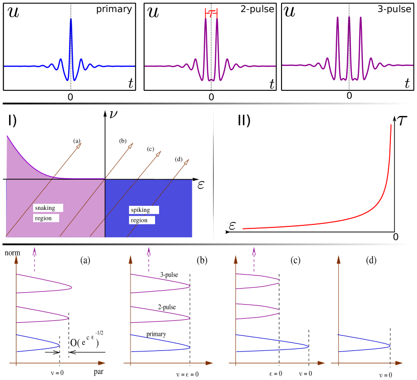
Figure 8: Qualitative summary of the results on bifurcation analysis of primary (blue) and multi-pulse (pink) homoclinic orbits. Top panel close to the codimension-two point $\varepsilon=\nu=0$. The middle panel shows the two main results: (I) the time of flight (distance peak to peak) in the 2-pulse solutions; (II) The region of existence of multi-pulse solution (snaking region), the sub-figures indicate the results of one-parameter continuation along each of the depicted paths (a)–(c).

Notice that curve (44) emanates from the codimension-two point $(\varepsilon,\nu)=(0,0)$. Thus two-pulse orbits are destroyed in a fold for positive $\nu$-values which, as $\varepsilon\to 0$, tends exponentially quickly to the same parameter value $\nu=0$ as the primary fold. It is in principle a straightforward argument to show that all $n$-pulse for $n>2$ should also be destroyed in this manner as $\nu$-increases (see path (a) in Figure. 8 panel I) and the respective one-parameter continuation sketch in the bottom panel).

We can now ask the question what happens to the same orbits as we move from path (a) to path (c) in Fig. 8 via path (b) which passes through the codimension-two point. On path (c) the multi-pulse orbits first cross $\varepsilon=0$ before reaching $\nu=0$ and therefore each multi-pulse orbit is destroyed via a bifurcation at which $\tau\to\infty$. This is a bifurcation in which the large pulse-like maxima become infinitely far seperated.

We should stress that there is no guarantee from this analysis that the two-pulse orbit that are connected globally to the primary via the homoclinic snake should be destroyed via this mechanism, it is just that all multi-pulse orbits that pass in the vicinity of the primary homoclinic orbit $\gamma$ inside the box B must be destroyed in this manner. Nevertheless, we note from the numerical results in the Sec.2 indicate that in both of the examples, the multi-pulse orbits within the homoclinic snake do indeed get destroyed at the Belyakov-Devaney transition via the mechanism we have just outlined. In particular, the bottom panel of Fig. 4 (see inset (c)), shows the one-parameter continuation of the two-pulse orbit. In that case, the bifurcation diagram exhibits the same behavior predicted by this analysis (cf. Fig. 8(c)), where the two-pulse homoclinic orbit terminates precisely at the Belyakov-Devaney transition.

4.2 Comparison with numerical results

In order to conclude the analysis, we shall compare the above quantitative predictions with numerical results obtained from the two example systems studied in Sec. 2. More precisely, we shall seek evidence for the scaling predictions (42) for the pulse-to-pulse seperation $\tau$, and (44)) for the the $\nu$-value of the fold as a function of $\varepsilon$.

We should stress at the outset that there extreme numerical difficulties with attempting such verification. As has been documented elsewhere, e.g [47, 57], it is a difficult numerical task to accurately compute a multi-pulse homoclinic in the limit (equivalent to $\varepsilon\to 0^{-}$ here) that the pulses become infinitely far seperated. The inherent problem is that two graphs of the primary orbit placed side by side with arbitrary seperation $\tau$ approximately solve the system up to an error that is exponentially small as $\tau\to\infty$. Hence any initial-value or boundary-value solver with finite precision is unable to distinguish true two-pulse orbits. For this reason, we have been unable to trace two-pulse orbits particularly far into the limit $\varepsilon\to 0^{-}$.

In each of the two examples, our numerical procedure was as follows. Using two-parameter continuation in Auto [29], we find accurately locate the codimension-two point at which there is a fold of the primary homoclinic orbit with respect to a parameter and simultaneous the imaginary part of the eigenvalues of the equilibrium vanish. We then compute the two-pulse orbit that is globally part of the homoclinic snake and follow the fold of this orbit in the same two parameters. Along this curve we monitor the eigenvalues of the equilibrium and define a parameter $\varepsilon$ as in the analysis such that the imaginary part of the eigenvalues are $\pm\sqrt{-\varepsilon}$. We then define a parameter that is equivalent to $\nu$ by projecting the displacement in the parameter plane to the curve on which the primary orbit has its fold, onto the the direction to curves $\varepsilon=$const. to be equivalent to $\nu$ from the analysis. The origin of $\nu$ In this manner we probe the region of the that is distinguished with a maroon star in the top panel of Figures 4 and 5, measuring as we do the distance between the two large peaks (equivalent to $\tau$ up to a constant).

The results for both models are summarized in Fig. 9. In both cases, for the numerical reasons outlined above, we find that the curve of folds of the two-pulse orbit fails to converge at some significant distance from the codimension-two point, equivalent to $\varepsilon=\mathcal{O}(1)$.

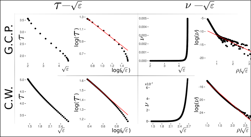
Figure 9: Comparing between the asymptotic predictions for $\tau$ (42) (Left side) and $\nu$ (44) (Right side) as a function of the eigenvalues and results of the numerical continuation. The Top (Bottom) half illustrates these results in the (G)eneralized (C)ell (P)olarity Model ((C)rime (W)ave model). Black points correspond to the results of the numerical continuation and the red lines represents the linear fit. See text for details.

The results for the pulse-to-pulse distance as a function of $\sqrt{|\varepsilon|}$ are presented in the left-hand panels of the Fig. 9. Not how, in both models, the time of flight $\tau$ increases algebraically as $\varepsilon$ tends to zero. Furthermore, considering the logarithm of (42), we obtain

(45) $$\log\tau=-c_{1}\log\sqrt{\varepsilon}+c_{2},\quad\text{ with }c_{1}=1\quad\mbox{and }c_{2}=\log\left[\pi\left(n+\frac{1}{4}\right)\right],$$

suggesting that, under this transformation, a linear model could be fit to the numerical results. Such a linear fit is indicated in the next right-most panels of the figure.

The third column of pabels in Fig. 9 shows numerical results for location of the $\nu$-value distance between the fold of the two-pulse and primary orbit. The exponential-like behavior exhibited by both models is apparent. By considering the logarithm of expression (44) one can obtain a straight line prediction on a log-log plot:

(46) $$\log\nu_{\rm fold}=-c_{3}\frac{\rho}{\sqrt{\varepsilon}}+c_{4},\quad\mbox{ with }c_{3}=2\pi\left(n+\frac{1}{4}\right),\quad c_{4}=\log(h\varphi\sin(\theta^{*})).$$

The final column shows that such a linear prediction can be observed in the limit of small $\sqrt{\varepsilon}$.

While these results are encouraging, there is little evidence that the constants $c_{1}$–$c_{4}$ match those of the theory. The constants found in the least-squares linear regression fits in Fig. 9 are given in Table 1. Note that As $\varepsilon\to 0$, in addition to observing the expected behaviors (i.e. $\tau\to\infty$ and $\nu\to 0$), we also can also see the transition between non-linear (large $\varepsilon$) to linear (smaller $\varepsilon$) regimes. These changes are more pronounced in the log and semi-log scales (cf. Figure 9). Since we are testing (45) and (46), we therefore used a sub-interval of $\varepsilon$ and $\rho/\varepsilon$, respectively. The rightmost column in Tables 1 (a) and (b) specifies the range used in each case.

(a) Prediction $\tau(\sqrt{\varepsilon})$	(b) Prediction $\nu(\sqrt{\varepsilon},\rho)$
Model $c_{1}$ $c_{2}$ $R^{2}$ Range G.C.P. 0.62 1.71 0.997 $\log\sqrt{|\varepsilon|}<1.4$ C.W. 0.62 1.84 0.999 $\log\sqrt{|\varepsilon|}<0.65$	Model $c_{3}$ $c_{4}$ $R^{2}$ Range G.C.P. 2.89 8.53 0.826 $\frac{\rho}{\sqrt{\varepsilon}}>$1 C.W. 6.89 7.73 0.990 $\frac{\rho}{\sqrt{\varepsilon}}>0.1$

Table 1: Linear regression of the numerical continuation results using the linear models for $\tau$ (45) (a) and $\nu$ (46) (b) respectively. The result of these linear regression have been illustrated in Figure 9.

The linear regression confirms that in each case we observe a linear behavior (see the $R^{2}$ values in Table 1). Additionally, the approximation for $c_{1}$ and $c_{2}$ in Table 1(a) are remarkably similar between models. However, the match to the theoretical value $c_{1}=1$ is poor, presumably because $\sqrt{\varepsilon}$ is still a long way from the limit $\varepsilon=0$ where the approximation is valid. In contrast, the $\nu-\varepsilon$ linear fit presents differences between $c_{3}$ and $c_{4}$.

5 Discussion

In this paper we have reported progress in the description of the transition between spike-like and localized patterned states in systems of reaction diffusion equations. That the scenario have been observed in two separate examples, suggest that this is a generic situation.

The key we have found to understanding the transition in both examples is that, in a two-parameter space, the localized-structure region is bisected by a line corresponding to the codimension-one Belyakov-Devaney transition. To that end we provided a partial unfolding of the codimension-two degeneracy where a fold of a primary homoclinic orbit coincides with the Belyakov-Devaney transition. By introducing two parameters, $\varepsilon$ controlling the linearization and $\nu$ controlling the primary homoclinic fold, we find the asymptotic scalings of how all subsidiary multi-pulse orbits are destroyed in a neighborhood in parameter space.

Our main contribution has been to find approximate expressions for the local and global Poincaré maps in a neigborhood of the degenerate homoclinic orbit we study. This is particularly challenging because of the lack of a closed form analytical expression for the local map, and because of the need to unfold the quadratic tangency in the global map in a generic way. We are unaware of any previous work that has attempted to unfold such a codimension-two singularity.

The main results of the analysis are summarized qualitatively in Fig. 8. In particular, according to (44), we find that the $\nu$-values of the folds of all the subsidiary orbits become exponentially close to that of the primary orbit as $\varepsilon\to 0$. This prediction from the analysis, and the prediction (42) on the rate of separation multi-pulses as $\varepsilon\to 0$ for $\nu<0$, were tested against two example systems and found to be consistent. Precise quantitative verification is problematic though due to inherent numerical difficulties in computing multi-pulse orbits close to the codimension-two point, as has been report elsewhere in this contex (see e.g. [47, 57]). Perhaps computation using arbitrary precision arithmetic might resolve this problem, but that is beyond the scope of the present work.

We should also point out that what we have found is not the only way that a homoclinic snake can become more complex than the simple picture in Figure. 2. A number of generic possibilities of the structure of homoclinic curves within the pinning region are analyzed in [43]. In essence what we have analyzed is a situation in which the left-hand fold of the snake in Figure. 2 crashes into another bifurcation. Another possibility is that the right-hand fold of the snake should approach the parameter value of the Turing bifurcation, which has been seen in a number of systems and also leads to $C$-shaped isolas. In contrast though all homoclinic orbits grow algebraic rather than exponential tails in this limit, rather than multi-pulses disappearing to infinity. Another possibility is that the left-hand folds of the snake coincide with a fold of the primary pattern forming periodic orbit. This situation was analyzed in [21] and leads to $S$-shaped isolas in which compound small and large pulses form defect mediated snaking [42].

It should also be stressed that all we have shown is the mechanism by which infinitely many multi-pulse homoclinic orbits are destroyed as a fold of a primary homoclinic orbit reaches a Belyakov-Devaney transition. However, there is no a priori reason that these orbits should be part of what was the homoclinic snake born at the codimension-two degenerate Turing bifurcation (the red circle in Figs. 4 and 5). In fact, the analysis of homoclinic snaking [56, 8, 43] occurs due to an unfolding of a heteroclinic orbit between a hyperbolic equilibrium and a generic saddle-like periodic orbit. In principle, as the equilibrium passes through a double-real-eigenvalue transition it remains hyperbolic and the dimensions of the stable and unstable manifolds in question do not change. It just seems that for the particular examples we have studied, the periodic orbit that is involved in the heteroclinic connection becomes the smaller-amplitude homoclinic orbit passing through the Belyakov-Devaney point. (See for example the bottom Figure. 4(c) in which the multi-pulse orbit being destroyed in the upper panel is actually a hybrid of the large-amplitude and the small-amplitude homoclinic orbit). Why this periodic orbit should become homoclinic is not clear. The question would seem to be tied up with an unfolding of the singular point in which there is a quadruple zero eigenvalue equilibrium in which the diffusion ratio is also zero (equivalent to $\gamma=\delta=0$ in our first example).

As further evidence of the ubiquity of what we have found here, forthcoming work will show that the same transition between spikes and localized patterns as analyzed here also occurs in a wide variety of Schnakenberg-type models in the presence of symmetry-breaking terms [3]. We also mention the related work [48] on the Lugiato-Lefever equation which has a related transition to the one here, but for which the fundamental codimension-two bifurcation has a different structure.

There remain many aspects of this problem that we have not fully analyzed, in addition to an unfolding of this singular codimension-two point. For example, there is more that can be said about the ordering of two-, three-, etc.- pulse orbits and prediction that the disappearance of multi-pulse orbits is via hybrids between the large and small-amplitude homoclinic orbits. The fact that the $W^{u}(0)$ is two-dimensional means that homoclinic orbits have a specific ordering and disappearance of certain orbits through a fold has implications on non-existence of certain other orbits at that parameter value. Extensive arguments of this nature were previously used in [13] in a related context.

References

- [1] T. Ackemenn and W. Firth, Chapter 6: Fundamentals and applications of spatial dissipative solitons in photonic devices, in Advances in Atomic Molecular and Optical Physics, vol. 57, Academic Press, 2009, pp. 323– 421.
- [2] N. Akhmediev and A. Ankiewicz, Dissipative Solitons, Springer-Verlag, Berlin, 2005. Lecture Notes in Physics.
- [3] F. Al Saadi, A. Champneys, and N. Verschueren, Universal structure of localized patterns in Schnackenberg-like models, 2020. In preparation.
- [4] J. Alexander, M. Grillakis, C. Jones, and B. Sandstede, Stability of pulses on optical fibers with phase-sensitive amplifiers, Z. Angew. Math. Phys., 48 (1997), pp. 175–192.
- [5] D. Avitabile, D. Lloyd, J. Burke, E. Knobloch, and B. Sandstede, To snake or not to snake in the planar Swift-Hohenberg equation, SIAM J. App. Dynamical Sys., 9 (2010), pp. 704–733.
- [6] I. V. Barashenkov, M. M. Bogdan, and V. I. Korobov, Stability diagram of the phase-locked solitons in the parametrically driven, damped nonlinear schrödinger equation, EPL, 15 (1991), p. 113.
- [7] I. V. Barashenkov, E. V. Zemlyanaya, and T. C. van Heerden, Time-periodic solitons in a damped-driven nonlinear schrödinger equation, Phys. Rev. E, 83 (2011), p. 056609.
- [8] M. Beck, J. Knobloch, D. Lloyd, B. Sandstede, and T. Wagenknecht, Snakes, ladders, and isolas of localized patterns, SIAM Journal on Mathematical Analysis, 41 (2009), pp. 936–972.
- [9] L. Belyakov, A case of the generation of a periodic orbit motion with homoclinic curves, Math. Notes, 15 (1980), pp. 336–341.
- [10] L. Belyakov, L. Glebsky, and L. Lerman, Abundance of stable stationary localized solutions to the generalized 1d Swift-Hohenberg equation, Comp. & Math. App., 34 (1997), pp. 253–266.
- [11] I. Bordeu, M. Clerc, R. Lefever, and M. Tlidi, From localized spots to the formation of invaginated labyrinthine structures in a Swift-Hohenberg model, Commun. Nonlin. Sci. Num. Sim., 29 (2015), pp. 482–487.
- [12] V. Breña–Medina and A. Champneys, Subcritical Turing bifurcation and the morphogenesis of localized patterns, Phys. Rev. E, 90 (2014), p. 032923.
- [13] B. Buffoni, A. Champneys, and J. Toland, Bifurcation and coalescence of a plethora of homoclinic orbits for a hamiltonian system, Journal of Dynamics and Differential Equations, 8 (1996), pp. 221–279.
- [14] J. Burke and J. Dawes, Localized states in an extended Swift-Hohenberg equation, SIAM J. Appl. Dyn. Sys., 11 (2012), pp. 261–284.
- [15] J. Burke and E. Houghton, S.M. amd Knobloch, Swift-Hohenberg equation with broken reflection symmetry, Phys Rev E, 80 (2009), p. Art. No:036202.
- [16] J. Burke and E. Knobloch, Snakes and ladders: Localized states in the Swift–Hohenberg equation, Physics Letters A, 360 (2006), pp. 681–688.
- [17] J. Burke and E. Knobloch, Homoclinic snaking: Structure and stability, Chaos, 17 (2007), p. art. no. 037102.
- [18] A. Champneys, Subsidiary homoclinic orbits to a saddle-focus for reversible systems, International Journal of Bifurcation and Chaos, 04 (1994), pp. 1447–1482.
- [19] A. Champneys, Homoclinic orbits in reversible systems and their applications in mechanics, fluids and optics, Physica D: Nonlinear Phenomena, 112 (1998), pp. 158 – 186.
- [20] A. Champneys, Homoclinic orbits in reversible systems II: Multi-bumps and saddle-centres., CWI Quarterly, 12 (1999), pp. 185–212.
- [21] A. Champneys, E. Knobloch, Y.-P. Ma, and T. Wagenknecht, Homoclinic snakes bounded by a saddle-center periodic orbit, SIAM J. Appl. Dyn. Sys., 11 (2012), pp. 1583–1613.
- [22] S. Chapman and G. Kozyreff, Exponential asymptotics of localised patterns and snaking bifurcation diagrams, Physica D, 238 (2009), pp. 319–354.
- [23] M. Clerc and C. Falcon, Localized patterns and hole solutions in one-dimensional extended systems, Physica A: Statistical Mechanics and its Applications, 356 (2005), pp. 48 – 53.
- [24] J. Dawes, Localized pattern formation with a large-scale mode: Slanted snaking, SIAM J. App. Dyn. Sys., 7 (2008), pp. 186–206.
- [25] J. Dawes, Modulated and localised states in a finite domain, SIAM J. Appl. Dyn. Syst., 8 (2009), pp. 909–930.
- [26] A. Dean, P. Matthews, S. Cox, and J. King, Exponential asymptotics of homoclinic snaking, Nonlinearity, 24 (2011), pp. 3323–3351.
- [27] R. Devaney, Homoclinic orbits in Hamiltonian systems, J. Diff. Eqns., 21 (1976), pp. 431–438.
- [28] R. Devaney, Blue sky catastrophes in reversible and Hamiltonian systems, Indiana Univ. Math. J., 26 (1977), pp. 247–263.
- [29] E. Doedel, A. Champneys, T. Fairgrieve, Y. Kuznetsov, B. Sandstede, and X. Wang, Auto 97: Continuation and bifurcation software for ordinary differential equations (with homcont), 2002. Technical report, Concordia University.
- [30] A. Doelman, T. J. Kaper, and P. A. Zegeling, Pattern formation in the one-dimensional gray - scott model, Nonlinearity, 10 (1997), p. 523.
- [31] A. Doelman and F. Veerman, An explicit theory for pulses in two component, singularly perturbed, reaction–diffusion equations, Journal of Dynamics and Differential Equations, 27 (2015), pp. 555–595, https://doi.org/10.1007/s10884-013-9325-2, https://doi.org/10.1007/s10884-013-9325-2.
- [32] M. Haragus and G. Iooss, Local Bifurcations, Center Manifolds, and Normal Forms in Infinite-Dimensional Dynamical Systems, Springer, 2011.
- [33] J. Harterich, Cascades of homoclinic orbits to a saddle focus equilibrium, Physica D, 112 (1998), pp. 187–200.
- [34] S. Houghton and E. Knobloch, Swift-Hohenberg equation with broken cubic-quintic nonlinearity, Phys Rev E, 84 (2011), p. Art. No:016204.
- [35] D. Iron, M. J. Ward, and J. Wei, The stability of spike solutions to the one-dimensional gierer–meinhardt model, Physica D: Nonlinear Phenomena, 150 (2001), pp. 25 – 62.
- [36] E. Knobloch, Spatial localization in dissipative systems, Annual Review of Condensed Matter Physics, 6 (2015), pp. 325–359.
- [37] J. Knobloch, T. Rieß, and M. Vielitz, Nonreversible homoclinic snaking, Dynamical Systems, 26 (2011), pp. 335–365.
- [38] G. Kozyreff and S. Chapman, Asymptotics of large bound state of localised structures, Physical Review Letters, 97 (2006), p. art.no.044502.
- [39] G. Kozyreff and S. Chapman, Analytical results for front pinning between an hexagonal pattern and a uniform state in pattern-formation systems, Phys. Rev. Lett., 111 (2013), p. art. no. 054501.
- [40] D. Lloyd, B. Sandstede, D. Avitabile, and A. Champneys, Localized hexagon patterns of the planar Swift-Hohenberg equation, SIAM J. Appl. Dyn. Syst., 7 (2008), pp. 1049–1100.
- [41] D. J. Lloyd and H. O’Farrell, On localised hotspots of an urban crime model, Physica D: Nonlinear Phenomena, 253 (2013), pp. 23 – 39.
- [42] Y.-P. Ma, J. Burke, and E. Knobloch, Defect-mediated snaking: A new growth mechanism for localized structures, Physica D., 239 (2010), pp. 1867–1883.
- [43] E. Makrides and B. Sandstede, Predicting the bifurcation structure of localized snaking patterns, Physica D, 26 (2014), pp. 59–78.
- [44] S. McCalla and B. Sandstede, Spots in the Swift-Hohenberg equation, SIAM J. Appl. Dyn. Syst., 12 (2013), pp. 831–877.
- [45] R. Moore and K. Promislow, Renormalization group reduction of pulse dynamics in thermally loaded optical parametric oscillators, Physica D, 206 (2005), pp. 62–81.
- [46] Y. Mori, A. Jilkine, and L. Edelstein-Keshet, Wave-pinning and cell polarity from a bistable reaction-diffusion system, Biophysical Journal, 94 (2008), pp. 3684 – 3697.
- [47] B. Oldeman, B. Krauskopf, and A. Champneys, Numerical unfoldings of codimension-three resonant homoclinic flip bifurcations, Nonlinearity, 14 (2001), pp. 597–621.
- [48] P. Parra-Rivas, D. Gomila, L. Gelens, and E. Knobloch, Bifurcation structure of localized states in the Lugiato-Lefever equation with anomalous dispersion, Physical Review E, 97 (2018), p. art. no. 042204.
- [49] H. Purwins, H. Bödeker, and S. Amiranashvili, Dissipative solitons, Advances in Physics, 59 (2010), pp. 485–701.
- [50] I. Rozada, S. J. Ruuth, and M. J. Ward, The stability of localized spot patterns for the brusselator on the sphere, SIAM Journal on Applied Dynamical Systems, 13 (2014), pp. 564–627.
- [51] M. Sevryuk, Reversible Systems, Springer, New York, 2009. Lecture Notes in Mathematics.
- [52] L. P. Shil’nikov, L. Shil’nokov Andrey, D. V. Turaev, and O. Chua, Leon, Methods of Qualitative Theory in Nonlinear Dynamics: Part I and II, World Scientific, 1998.
- [53] M. B. Short, M. R. D’Orsonga, V. B. Pasour, G. E. Tita, P. J. Brantingham, A. L. Bertozzi, and L. B. Chayes, A statistical model of criminal behavior, Mathematical Models and Methods in Applied Sciences, 18 (2008), pp. 1249–1267.
- [54] N. Verschueren, U. Bortolozzo, M. Clerc, and S. Residori, Chaoticon: localized pattern with permanent dynamics, Philosophical Transactions of the Royal Society of London A: Mathematical, Physical and Engineering Sciences, 372 (2014).
- [55] N. Verschueren and A. Champneys, A model for cell polarization without mass conservation, SIAM Journal on Applied Dynamical Systems, 16 (2017), pp. 1797–1830.
- [56] P. Woods and A. Champneys, Heteroclinic tangles and homoclinic snaking in the unfolding of a degenerate reversible Hamiltonian–Hopf bifurcation, Physica D: Nonlinear Phenomena, 129 (1999), pp. 147–170.
- [57] Y. R. Zelnik, H. Uecker, U. Feudel, and E. Meron, Desertification by front propagation?, Journal of Theoretical Biology, 418 (2017), pp. 27 – 35.