Understanding Behavior of Clinical Models under Domain Shifts

Abstract.

The hypothesis that computational models can be reliable enough to be adopted in prognosis and patient care is revolutionizing healthcare. Deep learning, in particular, has been a game changer in building predictive models, thus leading to community-wide data curation efforts. However, due to inherent variabilities in population characteristics and biological systems, these models are often biased to the training datasets. This can be limiting when models are deployed in new environments, when there are systematic domain shifts not known a priori. In this paper, we propose to emulate a large class of domain shifts, that can occur in clinical settings, with a given dataset, and argue that evaluating the behavior of predictive models in light of those shifts is an effective way to quantify their reliability. More specifically, we develop an approach for building realistic scenarios, based on analysis of disease landscapes in multi-label classification. Using the openly available MIMIC-III EHR dataset for phenotyping, for the first time, our work sheds light into data regimes where deep clinical models can fail to generalize. This work emphasizes the need for novel validation mechanisms driven by real-world domain shifts in AI for healthcare.

1. Introduction

The role of automation in healthcare and medicine is steered by both the ever-growing need to leverage knowledge from large-scale, heterogeneous information systems, and the hypothesis that computational models can actually be reliable enough to be adopted in diagnostics. Deep learning, in particular, has been a game changer in this context, given recent successes with both electronic health records (EHR) and raw measurements (e.g. ECG, EEG)  (Rajkomar et al., 2018),  (Rajan and Thiagarajan, 2018). While designing computational models that can account for complex biological phenomena and all interactions during disease evolution is not possible yet, building predictive models is a significant step towards improving patient care. There is a fundamental trade-off in predictive modeling with healthcare data. While the complexity of disease conditions naturally demands expanding the number of predictor variables, this often makes it extremely challenging to identify reliable patterns in data, thus rendering the models heavily biased. In other words, despite the availability of large-sized datasets, we are still operating in the small data regime, wherein the curated data is not fully representative of what the model might encounter when deployed.

In this paper, we consider a variety of population biases, label distribution shifts and measurement discrepancies that can occur in clinical settings, and argue that evaluating the behavior of predictive models in light of those shifts is crucial to understanding strengths and weaknesses of predictive models. To this end, we consider the problem of phenotyping using EHR data, characterize different forms of discrepancies that can occur between train and test environments, and study how the prediction capability varies across these discrepancies. Our study is carried out using the openly available MIMIC-III EHR dataset (Johnson et al., 2016) and the state-of-the-art deep ResNet model (Bai et al., 2018). The proposed analysis provides interesting insights about which discrepancies are challenging to handle, which in turn can provide guidelines while deploying data-driven models.

2. Dataset Description

All experiments are carried out using the MIMIC-III dataset (Johnson et al., 2016), the largest publicly available database of de-identified EHR from ICU patients. It includes a variety of data types such as diagnostic codes, survival rates, length of stay etc., yielding a total of $76$ measurements. For our study, we focus on the task of acute care phenotyping that involves retrospectively predicting the likely disease conditions for each patient given their ICU measurements. Preparation of such large heterogeneous records involve organizing each patient’s data into episodes containing both time-series events as well as episode-level outcomes like diagnosis, mortality etc. Phenotyping is typically a multi-label classification problem, where each patient can be associated with several disease conditions. The dataset contains $25$ disease categories, $12$ of which are critical such as respiratory/renal failure, $8$ are chronic conditions such as diabetes, atherosclerosis, with the remaining $5$ being ’mixed’ conditions such as liver infections. Note that, in our study, we reformulate the phenotyping problem as a binary classification task of detecting the presence or absence of a selected subset of diseases.

Figure 1. Constructing disease landscapes: Using information decomposition on the MIMIC-III EHR dataset reveals the grouping of disease outcomes.

3. Analysis of Deep Clinical Models

Clinical time-series modeling broadly focuses on problems such as anomaly detection, tracking progression of specific diseases or detecting groups of diseases. Deep learning provides a data-driven approach to exploiting relationships between a large number of input measurements while producing robust diagnostic predictions. In particular, Recurrent Neural Networks (RNN) was one of the earlier solutions for dealing with sequential data in tasks such as discovering phenotypes and detecting cardiac diseases (Rajan and Thiagarajan, 2018), etc. The work by (Rajkomar et al., 2018) extensively benchmarked the effectiveness of deep learning techniques in analyzing EHR data. More recently, convolutional networks (Bai et al., 2018), and attention models (Song et al., 2018) have become highly effective alternatives to sequential models. In particular, deep Residual Networks with $1D$ convolutions (ResNet-$1D$), have produced state-of-the-art performance in many clinical tasks (Bai et al., 2018). Hence, in this work, all studies are carried out using this architecture.

Architecture: We use a ResNet-$1D$ model with $7$ residual blocks which transform the raw time-series input into feature representations. Each residual block is made up of two 1-D convolution and batch normalization layers with a kernel size of $3$ and $64$ or $256$ filters, a dropout and a leaky-ReLU activation layer. Further, a $1-D$ max pooling layer is used after the third and seventh residual blocks to aggregate the features. Additional parameters include: an Adam optimizer with a learning rate of $0.001$, and a batch size of $128$ with an equal balance of positive and negative samples.

Proposed Work: An important challenge with the design of deep clinical models is the lack of a holistic understanding of their behavior under the wide-range of discrepancies that can occur between train and test environments. In particular, we consider the following domain shifts – (i) population biases such as age, gender, race etc.; (ii) label distribution shifts such as novel disease conditions at test time, presence of combinations of observed diseases etc.; and (iii) measurement discrepancies such as noisy labels, missing measurements, variations in sampling rate etc. Understanding how much these discrepancies impact a model’s generalization performance is critical to qualitatively understanding its strengths and expected regimes of failure, and thus provide guidelines for effective deployment. Conceptually, this amounts to quantifying the prediction uncertainties arising due to the lack of representative data and inherent randomness from clinical data.

4. Characterizing Domain Shifts

In this section, we describe our approach for emulating a variety of domain shifts that commonly occur in a clinical setting, which will be then used for evaluating the deep 1D-ResNet model in the next section. For each of the cases, we construct a source and a target dataset, where the data samples are chosen based on a discrepancy-specific constraint (e.g. gender distribution, males used in source and females in target). The positive class corresponds to the presence of a selected subset of diseases (e.g. organ specific conditions), while the negative class indicates their absence in the patients. Note, we ensured that the resulting datasets are balanced, and had positive-negative split of $\sim 60\%-40\%$. Before we describe the different discrepancies considered in our study, we will briefly discuss the information decomposition technique (Steeg and Galstyan, 2016) that will be used to explore the landscape of diseases in order to pick a subset of related conditions for defining the positive class.

Exploring Disease Landscapes: We utilize information sieve (Steeg and Galstyan, 2016), a recent information-theoretic technique for identifying latent factors in data that maximally describe the total correlation between variables. Denoting a set of multivariate random variables by $\tilde{X}=\{\tilde{X}_{i}\}_{i=1}^{d}$, dependencies between the variables can be quantified using the multivariate mutual information, also known as total correlation (TC), which is defined as

(1) $$TC(\tilde{X})=\sum_{i=1}^{d}H(\tilde{X}_{i})-H(\tilde{X}),$$

where $H(\tilde{X}_{i})$ denotes the marginal entropy. This quantity is non-negative and zero only when all the $\tilde{X}_{i}$’s are independent. Further, denoting the latent source of dependence in $\tilde{X}$ by $\tilde{Z}$, we can define the conditional $TC(\tilde{X}|\tilde{Z})$, i.e., the residual total correlation after observing $\tilde{Z}$. Hence, we solve the problem of searching for $\tilde{Z}$ that minimizes $TC(\tilde{X}|\tilde{Z})$. Equivalently, we can define the reduction in $TC$ after conditioning on $\tilde{Z}$ as $TC(\tilde{X};\tilde{Z})=TC(\tilde{X})-TC(\tilde{X}|\tilde{Z})$. The optimization begins with $\tilde{X}$, constructs $\tilde{Z}_{0}$ to maximize $TC(\tilde{X};\tilde{Z}_{0})$. Subsequently, it computes the remainder information not explained by $\tilde{Z}_{0}$, and learns another factor, $\tilde{Z}_{1}$, that infers additional dependence structure. This procedure is repeated $k$ times until the entirety of multivariate mutual information in $\tilde{X}$ is explained.

Denoting a labeled dataset using the tuple $(\mathbf{X},\mathbf{Y})$, where $\mathbf{X}\in\mathbb{R}^{N\times D}$ is the input data with $D$ variables, and $\mathbf{Y}\in\mathbb{R}^{N\times d}$ is the label matrix with $d$ different categories, we use information sieve to analyze the outcome variables. In other words, we identify latent factors to describe the total correlation in $\mathbf{Y}$ and the resulting hierarchical decomposition is referred as the disease landscape. The force-based layout in Figure 1 provides a holistic view of the landscape for the entire MIMIC-III dataset. Here, each circle corresponds to a latent factor and their sizes indicate the amount of total correlation explained by that factor, and the thickness of edges reveal contributions of each outcome variable to that factor.

4.1. Population Biases

Clinical datasets can be imbalanced as to population characteristics.

(i) Age: (a) Older-to-Younger: Source comprises of patients who are $60$ years and above, and the target includes patients who are below $60$ years of age; (b) Younger-to-Older: This represents the scenario with source containing patients younger than $60$. Once the population is divided based on the chosen age criteria, we pick a cluster of diseases in the source’s disease landscape as the positive class. However, due to the domain shift, the landscape can change significantly in the target. Hence, in the target, we recompute the landscape and consider the source conditions as well as diseases strongly correlated to any of those conditions as positive.

(ii) Gender: Similar to the previous case, we emulate two cases, Male-to-Female, i.e. source data consists only of patients who identify as male and target has only patients who are female. While, the second scenario Female-to-Male is comprised of female-only source data and male-only target data.

(iii) Race: We emulate White-to-Minority, that contains prevalent racial groups such as white American, Russian, and European in the source, while constructing the target domain comprising of patients belonging to minority racial groups like Hispanic, South America, African, Asian, Portuguese, and others marked as unknown.

4.2. Label Distribution Shifts

When models are trained to detect the presence of certain diseases, they can be ineffective when novel disease conditions or variants of existing conditions, previously unseen by the model, appear.

(i) Novel Diseases at Test Time: (a) Resp-to-CardiacRenal: In the source, we detect the presence or absence of diseases from cluster $1$ (Figure 1), while the target requires detection of the presence of at least one of the conditions from cluster $1$ or unobserved conditions in cluster $0$; (b) Cerebro-to-CardiacRenal: This is formulated as detecting diseases from cluster $2$ in the source dataset, while expanding the disease set in the target by including cluster $0$.

(ii) Dual-to-Single: As a common practice, lab tests for two diseases could be conducted together based on the likelihood of them co-occurring, giving rise to a dataset containing patients with both diseases. However, one would expect to detect the presence of even one of those diseases. Here, source includes patients associated with two disease conditions simultaneously, while target includes patients who present only one of the two. Note, we do not construct the landscapes for this case, instead, we divide patients into four groups, namely: those that have only cardiac diseases, only renal diseases, neither cardiac or renal diseases, and, both cardiac and renal diseases, and build the source-target pair.

(iii) Single-to-Dual: Similar to the previous case, an alternate situation could occur with models having to adapt to predicting patients that have two diseases, while having been trained on patients who were diagnosed with only one of them. Such a scenario is explored using a source dataset comprising of patients diagnosed as having either cardiac only or respiratory only disease, and a target dataset with patients that have both diseases.

4.3. Measurement Discrepancies

(i) Noisy Labels: Variabilities in diagnoses between different experts is common in clinical settings (Valizadegan et al., 2013). Consequently, it is important to understand the impact of those variabilities on behavior of the model, when adopted to a new environment. We extend the Resp-to-CardiacRenal case by adding uncertainties to the diagnostic labels in the source data and study its impact on the target. In particular, we emulate two such scenarios by randomly flipping $10$% and $20$% of the labels respectively.

(ii) Sampling Rate Change: Another typical issue with time-series data is the variability in sampling rates. We create a source-target pair based on the Resp-to-CardiacRenal scenario with measurements collected at different sampling rates. The source uses samples at every $96$ hours while the target is sampled at $48$ hours.

(iii) Missing Measurements: Clinical time-series is plagued by missing measurements during deployment, often due to resource or time limitations. We emulate this discrepancy based on the Dual-to-Single scenario, wherein we assume that the set of measurements, pH, Temperature, Height, Weight, and all Verbal Response GCS parameters, were not available in the target dataset. We impute the missing measurements with zero and this essentially reduces the dimensionality of valid measurements from $76$ to $41$ in the target.

5. Empirical Results

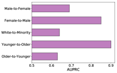
(a) Population Biases

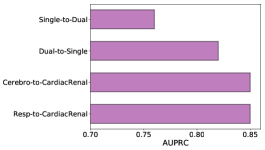
(b) Label Distribution Shifts

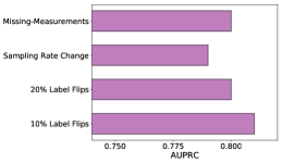
(c) Measurement Discrepancies

Figure 2. Results from our empirical study on generalizability of the ResNet-$1D$ model with complex domain-shifts.

Table 1. Disease conditions considered in source-target pairs for scenarios where the model demonstrated poor generalization.

Shift	Source Diseases	Target Diseases
Older-to-Younger	Coronary atherosclerosis, Disorders of lipid metabolism, Essential hypertension	Coronary atherosclerosis, Disorders of lipid metabolism, Essential hypertension, Chronic kidney disease, Secondary hypertension
Male-to-Female	Dysrhythmia, Congestive heart failure	Dysrhythmia, Congestive Heart Failure, Coronary atherosclerosis
White-to-Minority	Dysrhythmia, Conduction disorder, Congestive heart failure	Dysrhythmia, Conduction disorder, Congestive heart failure, Chronic kidney disease, Secondary hypertension, Diabetes
Single-to-Dual	Cardiac-only or Renal-only	Both Cardiac and Renal Diseases

In this section, we present empirical results from our study – performances of the ResNet-$1D$ model trained on the source data when subjected to perform under a variety of discrepancies. Following common practice, we considered the weighted average AUPRC metric. Figure 2 illustrates the performance of the ResNet-$1D$ model for the three categories of discrepancies. We report the weighted AUPRC score for each of the cases by training the model on source and testing on the target. Broadly, these results characterize the amount of uncertainty for even a sophisticated ML model, when commonly occurring discrepancies are present.

The first striking observation is that population bias leads to significant performance variability, wherein the AUPRC score varies in a wide range between $0.65$ and $0.9$. Note that, by identifying disparate sets of disease conditions, the reported results correspond to the worst-case performance for each scenario. In particular, we observe that the racial bias White-to-Minority, the gender bias Male-to-Female, and the age bias Older-to-Younger demonstrate challenges in generalization. This sheds light on the fact that manifestation of different disease conditions in the younger population shows higher variability compared to older patient groups, and hence a model overfit to the older case does not generalize to the former. Table 1 lists the set of source and target diseases for the cases with poor generalization. In the Older-to-Younger scenario, it is observed that the disease landscape of older patients reveals strong co-occurrence between Coronary atherosclerosis, Disorders of lipid metabolism, and Essential hypertension. In contrast, when one of these diseases occur in younger patients, it is often accompanied by other conditions such as Secondary hypertension and Chronic kidney disease. This systematic shift challenges pre-trained models to generalize well to the target. Similarly, in the case of White-to-Minority, while Congestive Heart Failure commonly manifests with Dysrhythmia in a predominantly white population, additional conditions such as Secondary Hypertension and Diabetes co-occur among minorities.

In the case of label distribution shifts, when there is no population bias, surprisingly the model is able to generalize well even when unseen disease conditions are present in the target. This is evident from the high AUPRC scores for both Resp-to-CardiacRenal and Cerebro-to-CardiacRenal. However, the EHR signatures for patients that present subsets or supersets of diseases observed in source are challenging to handle. In particular, detecting the presence of both cardiac and renal conditions using source data with patients who had only either of the diseases as in Single-to-Dual. This clearly shows the inherent uncertainties in biological systems (often referred to as aleatoric uncertainties) that cannot be arbitrarily reduced by building sophisticated ML models.

Finally, with respect to measurement discrepancies, it is widely believed that quality of labels in the source data is highly critical. However, surprisingly, we observe that with limited noise in the labels (10% Label Flips), the performance degradation is minimal. However, as the amount of noise increases (20% Label Flips), there is further degradation. Another important observation is that sampling rate change has a negative effect on the generalization performance and simple imputation does not suffice (we adopt a strategy where value from the last time-step is repeated). In comparison, the model is fairly robust to missing measurements.

References

- (1)
- Bai et al. (2018) Shaojie Bai, J. Zico Kolter, and Vladlen Koltun. 2018. An Empirical Evaluation of Generic Convolutional and Recurrent Networks for Sequence Modeling. arXiv:1803.01271 (2018).
- Johnson et al. (2016) Alistair EW Johnson, Tom J Pollard, Lu Shen, Li-wei H Lehman, Mengling Feng, Mohammad Ghassemi, Benjamin Moody, Peter Szolovits, Leo Anthony Celi, and Roger G Mark. 2016. MIMIC-III, a freely accessible critical care database. Scientific data 3 (2016).
- Rajan and Thiagarajan (2018) Deepta Rajan and Jayaraman J Thiagarajan. 2018. A Generative Modeling Approach to Limited Channel ECG Classification. arXiv preprint arXiv:1802.06458 (2018).
- Rajkomar et al. (2018) Alvin Rajkomar, Eyal Oren, Kai Chen, Andrew M Dai, Nissan Hajaj, Michaela Hardt, Peter J Liu, Xiaobing Liu, Jake Marcus, Mimi Sun, et al. 2018. Scalable and accurate deep learning with electronic health records. npj Digital Medicine 1, 1 (2018), 18.
- Song et al. (2018) Huan Song, Deepta Rajan, Jayaraman J Thiagarajan, and Andreas Spanias. 2018. Attend and Diagnose: Clinical Time Series Analysis using Attention Models. Proceedings of AAAI 2018 (2018).
- Steeg and Galstyan (2016) Greg Ver Steeg and Aram Galstyan. 2016. The information sieve. In Proceedings of the 33rd International Conference on International Conference on Machine Learning-Volume 48. JMLR. org, 164–172.
- Valizadegan et al. (2013) Hamed Valizadegan, Quang Nguyen, and Milos Hauskrecht. 2013. Learning classification models from multiple experts. Journal of biomedical informatics 46, 6 (2013), 1125–1135.