Extended $\Lambda$CDM model

Abstract

In this work we discuss a general approach for the dissipative dark matter considering a nonextensive bulk viscosity and taking into account the role of generalized Friedmann equations. This generalized $\Lambda$CDM model encompasses a flat universe with a dissipative nonextensive viscous dark matter component, following the Eckart theory of bulk viscosity. In order to compare models and constrain cosmological parameters, we perform Bayesian analysis using one of the most recent observations of Type Ia Supernova, baryon acoustic oscillations, and cosmic microwave background data.

I Introduction

The observable Universe is undergoing a current process of accelerated expansion being well explained through the standard $\Lambda$CDM model. Although this model provides a good fit to the data, there are some drawback issues which need to be investigated, e.g., the discrepancy between the theoretical expectation value and the observational one of the cosmological constant weinberg89 . From the observational standpoint, there is a tension associated with the measurement of the current value of the Hubble parameter when is used the power spectrum amplitude or considered the measurements of the matter density parameter (see, h0tension and the references therein for details). These issues also have motivated alternative models in order to study the Universe. In this concern, cosmological models have been addressed, either using extended general relativity extendedGR , or providing dark energy models DE . Some thermodynamical aspects, based on the scalar-tensor extension of the $\Lambda$CDM model has also been presented as an argument for an extended model Algoner16 .

On the other hand, an extension of the usual Boltzmann-Gibbs Theory has been proposed in order to address the so-called complex systems tsallis-review . In short, the formalism considers the entropy formula as a nonextensive quantity where there is a parameter $q$ that measures the degree of nonextensivity. The Tsallis nonextensive statistics has been successfully applied in many physical problems tsallis-review . This formalism was applied in cosmology scenarios, for example, entropic cosmology for a generalized black hole entropy komatsu , black holes formation 25 ; 27 and the modified Friedmann equations using the Verlinde theory 28 . Another direct application is the connection between dissipative processes and nonextensive statistics 29 ; 30 . The mechanism behind this connection is based on so-called nonextensive/dissipative correspondence (NexDC). The idea of the NexDC is associated with the microscopic description of the fluid through the Tsallis distribution function which captures strong statistical correlation among the 4-momenta of the particles 31 ; 32 . The NexDC mechanism has been implemented in cosmology to describe a viscous dark matter 30 . By assuming the cosmological principle, dissipative processes such as shear and heat conduction are excluded, thus, in a homogeneous and isotropic background, only bulk viscosity is allowed for cosmic fluids. In Ref. 2 , the author derived the standard theory for relativistic bulk viscosity, and some years later, connection with cosmology was derived by Weinberg, Ellis and others 3 ; 4 ; 5 ; 6 ; 7 . The introduction of bulk viscosity into cosmology has been investigated from different standpoints. For instance, cosmological models with bulk viscosity can be interpreted as an effect of creation of particles 7-1 ; 7a (see, e.g., 8 ; 9 ; 10 ; 11 ; 12 ; 13 ; 14 ; 15 ; 16 ; 17 ; 18 ; bulk and the references therein for many connections between bulk viscosity and cosmology).

An issue which can be addressed, in the alternative viewpoint of the $\Lambda$CDM model, is related to a general framework which captures the role of the microscopic statistical correlations (nonextensive effects) introduced through the extension from the Maxwell-–Boltzmann–-Juttner statistics 31 ; 32 . Here, we propose a nonextensive $\Lambda$CDM model, we are taking into account an extension of standard model based on the nonextensive effects under the equipartition law of energy, as well as an interpretation of viscous dark matter through the NexDC 30 . By assuming the Universe composed of nonextensive dissipative process (bulk viscosity), the core of the model follows of implementation of the nonextensive effect through the Verlinde theory 19 ; 20 ; 21 . From a dynamical standpoint, these effects will provide a new gravitational dynamics linked to generalized Friedmann equations. The physical motivation for the formulation of this extended model is associated with microscopic statistical correlations captured by the nonextensive framework tsallis-review . We test the observational viability of this model performing Bayesian model selection analysis using the most recent observations of Type Ia Supernova, baryon acoustic oscillations, and cosmic microwave background data.

This paper is organized as follows. In section II we deduce modified Friedmann equations introducing the nonextensive effect through Verlinde theory. In section III we present the extended $\Lambda$CDM model. In section IV, using Type Ia Supernova (SN Ia), baryon acoustic oscillations (BAO) and first acoustic peak in cosmic microwave background (CMB) data, we implement Bayesian analysis and compare our model with $\Lambda$CDM to test the viability of the model. Finally, in section V, we summarize the main results.

II Friedmann Equations for dissipative processes

Let us derive the extended equations governing the dynamical evolution of the Friedmann-Lemaitre-Robertson-Walker (FLRW) universe, from the entropic force standpoint, and taking into account the nonextensive equipartition law of energy, the Unruh temperature, and a new interpretation for the viscous fluid. Following similar arguments of Ref. 21 , the FRLW metric is given by

$$ds^{2}=-dt^{2}+a^{2}(t)(dr^{2}+r^{2}d\Omega^{2}),$$ (1)

where $a(t)$ is the scale factor of the Universe. By using the results of Ref. 19 , let us consider a compact spatial region $\mathcal{W}$ with a compact boundary $\mathcal{\partial W}$, which is a sphere with physical radius $\tilde{r}=ar$. Here, the compact boundary $\mathcal{\partial W}$ acts as the holographic screen. By holographic principle, the number of bits on the screen is assumed as

$$N=\frac{A}{G},$$ (2)

where $A$ is the area of the screen. Assuming that the temperature $T$ on the holographic screen is related to the total energy through the nonextensive equipartition law of energy 33

$$E_{q}=\frac{N}{5-3q}T,$$ (3)

where $N$ is the number of bits on the screen.

Furthermore, we consider as a source of the FLRW universe, a fluid with nonextensive bulk viscosity. In this regards, the momentum-energy tensor reads 30

$$T_{q}^{\mu\nu}=T_{q=1}^{\mu\nu}+(q-1)\Delta T^{\mu\nu},$$ (4)

where $T_{q=1}^{\mu\nu}$ is momentum-energy tensor of perfect fluid and $\Delta T^{\mu\nu}$ is derived of the Eckart theory, being given by

$$\Delta T^{\mu\nu}=\Pi h^{\mu\nu}.$$ (5)

Here, $h^{\mu\nu}=g^{\mu\nu}+u^{\mu}u^{\nu}$ is the usual projector onto the local rest space of $u^{\mu}$ (four-velocity) and $g^{\mu\nu}$ is the metric. $\Pi$ is the bulk viscous pressure, which depends on the bulk viscosity coefficient and the Hubble parameter, i.e. $\Pi=-3\xi_{q}H$ 30 . By choosing a reference frame in which the hydrodynamics four-velocity $u^{\mu}$ is unitary, $u^{\mu}u_{\mu}=-1$, and replacing the Eq.(5) into Eq.(4), we obtain

$$T_{q}^{\mu\nu}=(\rho+P_{\text{eff}})u^{\mu}u^{\nu}+P_{\text{eff}}g^{\mu\nu},$$ (6)

where $\rho$ is the energy density, $P_{\text{eff}}=p_{k}+\Pi$, where $p_{k}$ is the kinetic pressure (equilibrium pressure) and $\Pi=-3(q-1)\xi H$. By applying the covariant derivative in Eq.(6) provides

$$\dot{\rho}+3H(\rho+p_{k})-9H^{2}\xi_{q}=0,$$ (7)

where $\xi_{q}=(q-1)\xi$.

The acceleration for a comoving observer at $r$ (at the place of screen) is given by 21 ,

$$a_{r}=-\frac{d^{2}\tilde{r}}{dt^{2}}=-\ddot{a}r.$$ (8)

This acceleration is caused by the matter in the spatial region enclosed by holographic screen. The Unruh formula relates the temperature on the screen to an acceleration. The relation should be understood as a formula for the temperature which is related to the acceleration. In this matter, the Unruh temperature is

$$T=\frac{a_{r}}{2\pi}.$$ (9)

From the special relativity standpoint, we use $E=\mathcal{M}$ with $\mathcal{M}$ being the active gravitational mass, which is related to the production of the acceleration. As is well known, this is called Tolman-Komar mass, defined by

$$\mathcal{M}=2\int_{\mathcal{W}}dV\Big{(}T^{\mu\nu}-\frac{1}{2}Tg^{\mu\nu}\Big{)}u_{\mu}u_{\nu}.$$ (10)

Here, by using momentum-energy tensor, given by Eq.(6), its trace and the normalization condition $u^{\mu}u_{\mu}=-1$ as well as considering that the active gravitational mass is measured by a comoving observer, we obtain

$$\mathcal{M}=\frac{4\pi}{3}\tilde{r}^{3}(\rho+3p_{k}+\Pi),$$ (11)

where $\tilde{r}=a(t)r$ and $\Pi$ is the bulk viscous pressure (bulk viscosity). Thus, from Eqs. (2), (3), (9), (11) and the energy-mass relation, it is possible to show that

$$\frac{\ddot{a}}{a}=-\frac{4\pi}{3}\left(\frac{5-3q}{2}\right)G(\rho+3p_{k}+\Pi),$$ (12)

This is the acceleration equation for the dynamical evolution of the FRLW universe. Multiplying $\dot{a}a$ on both sides of Eq.(12) and using the continuity Eq.(7), we obtain the extended Friedmann equations

$$H^{2}=\frac{8\pi G}{3}\rho\left(\frac{5-3q}{2}\right)-\frac{k}{a^{2}},$$ (13)

where $k$ is an integration constant which is identified as the spatial curvature in the region $\mathcal{W}$ in the theory of general relativity. The values for curvature are the well known, $k=-1,0,1$, open, closed, flat FRLW universe, respectively. Universe without nonextensivity ($q=1$), we recovered the standard Friedmann equations.

III Dynamics of Nonextensive Viscous Dark Matter

Following the modified Friedmann equations deduced in the previous section, let us address the main contributions to the total momentum-energy tensor of the cosmic fluid, i.e., the baryonic matter, the cosmological constant and the nonextensive viscous dark matter 30 . As the energy conservation for each component of the cosmic fluid is individually conserved, we obtain

$$\dot{\rho}_{i}+3H(\rho_{i}+p_{i})=0,$$ (14)

where $i$ corresponds baryonic matter (b), radiation (r) or cosmological constant ($\Lambda$). The conservation of nonextensive viscous dark matter component is given by

$$\dot{\rho}_{dm}+3H(\rho_{dm}+p_{dm}^{eff})=0,$$ (15)

in which $\rho_{dm}$ is the energy density and the effective pressure is

$$p_{dm}^{eff}=p_{k}+\Pi,$$ (16)

where $p_{k}$ is equilibrium pressure (for cold dark matter $p_{k}=0$) and $\Pi=-3\xi_{q}H$ is the pressure from the nonextensive bulk viscosity. The equation of state, Eq.(16) is a consequence of the nonextensive effect, where in the limit $q\rightarrow 1$, the viscous pressure becomes null 30 . The choice of bulk viscosity coefficient $\xi_{q}$ seems to be an important aspect for any viscous model. As is well known, the bulk viscosity coefficient $\xi_{q}$ depends on the ratio between the density of viscous dark matter fluid at any redshift and the one today 16 ; 17 ; 18

$$\xi_{q}=\xi_{q0}\Big{(}\frac{\rho_{dm}}{\rho_{dm0}}\Big{)}^{\alpha},$$ (17)

where $\xi_{q0}$ and $\alpha$ are constants and $\rho_{dm0}$ is the density of viscous dark matter fluid today. Note that the present viscosity is given by the parameter $\xi_{q0}$ 30 . For fixing values, $\alpha=0$ and $\alpha=-1/2$, the Integrated Sachs-Wolfe effect (ISW) problem of these viscous cosmologies models is alleviated 16 ; 18 . The values for $\alpha$ above have a physical interpretation: the lower value means a constant bulk viscosity coefficient and the upper means, the bulk viscous fluid corresponds to the total energy. We will investigate both situations, $\alpha=0$ and $\alpha=-1/2$, where it will be denoted by models I and II, respectively.

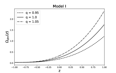
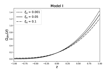
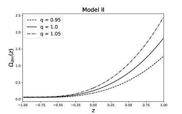
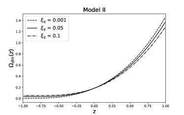
Figure 1: Evolution of nonextensive viscous dark matter parameter for selected values of $q$ and $\xi_{q}$. Here we have assumed $\Omega_{\Lambda 0}=0.70,\Omega_{b0}=0.046,\Omega_{r0}=8.5\times 10^{-5}.$

The Hubble expansion rate $H$ is given in terms of the fractional energy densities $\Omega_{i}$, where the subscript $i$ corresponds to each fluid,

$$\frac{H^{2}(z)}{H^{2}_{0}}=\left(\frac{5-3q}{2}\right)\Big{[}\Omega_{b0}(1+z)^{3}+\Omega_{r0}(1+z)^{4}$$ (18)

$$+\Omega_{dm}(z)+\Omega_{\Lambda}\Big{]},$$

In order to determine the function $\Omega_{dm}$, let us provide the nonextensive bulk viscosity coefficient and solve its conservation equation. For both models, the conservation equations for the nonextensive viscous dark matter fluid are given by

$$\frac{d\Omega_{dm}}{dz}= \frac{3\Omega_{dm}}{1+z}-\frac{\xi_{q}}{1+z}\Big{[}\frac{5-3q}{2}\Big{(}\Omega_{b0}(1+z)^{3}$$ (19)

$$+\Omega_{r0}(1+z)^{4}+\Omega_{dm}+\Omega_{\Lambda}\Big{)}\Big{]}^{1/2},$$

$$\frac{d\Omega_{dm}}{dz}= \frac{3\Omega_{dm}}{1+z}-\frac{\xi_{q}}{1+z}\Omega_{dm}^{-1/2}\Omega_{dm0}^{1/2}\Big{[}\frac{5-3q}{2}\Big{(}\Omega_{b0}(1+z)^{3}$$ (20)

$$+\Omega_{r0}(1+z)^{4}+\Omega_{dm}+\Omega_{\Lambda}\Big{)}\Big{]}^{1/2},$$

respectively. The bulk viscosity constant reads

$$\xi_{q}=\frac{24\pi G\xi_{q0}}{H_{0}},$$ (21)

being valid for both models. The initial condition for Eqs. (19) and (20) is $\Omega_{dm}(0)=\frac{2}{5-3q}-\Omega_{b0}-\Omega_{r0}-\Omega_{\Lambda}$. The Fig. 1 shows the evolution from the nonextensive dark matter density parameter for both models considering some selected values of $q$ and $\xi_{q}$. For different values of $q$ (with fixed viscosity, $\xi_{q}=0.1$), both models have a similar evolution. The models converge for a similar behavior in the future. And for different values of $\xi_{q}$ (with the parameter of nonextensivity fixed, $q=0.95$), there is a small difference in the evolution at high redshifts. It is worth noting that the nonextensivity is associated with the dynamics of the universe through the extended Friedmann equations and with the microscopic approach for the thermodynamics of the viscous dark matter. In particular, when $q\longrightarrow 1$, $\Lambda$CDM model is recovered. In the next section, we will use cosmological observations in order to obtain constraints on the parameters $\xi_{q}$, $q$ and $\Omega_{\Lambda}$.

IV Bayesian Analysis

Here, we will obtain the constraints of the parameters space and compare our model with $\Lambda$CDM by performing a Bayesian statistical analysis based on the presented data. In recent years, Bayesian analysis has been widely used to study and compare cosmological models bethoven ; simony ; maria ; uendert ; antonella . The posterior distribution $P(\Theta|D,M)$ is written in terms of the likelihood, $\mathcal{L}(D|\Theta,M)$, the prior, $\pi(\Theta|M)$, and Bayesian evidence or marginal likelihood $\mathcal{E}(D|M)$ as

$$P(\Theta|D,M)=\frac{\mathcal{L}(D|\Theta,M)\pi(\Theta|M)}{\mathcal{E}(D|M)},$$ (22)

where $\Theta$ denotes the parameters set, $D$ the cosmological data and $M$ the model. The Bayesian evidence, $\mathcal{E}$, should be irrelevant in the context of the parameter estimation, however one is essential in order to compare models based on the data. The evidence can be written in the continuous parameter space $M$ as

$$\mathcal{E}=\int_{M}\mathcal{L}(D|\Theta,M)\pi(\Theta|M)d\Theta.$$ (23)

In order to compare two models, $M_{i}$ and $M_{j}$, both describing the same phenomenon, we compute the ratio of the posterior probabilities, or posterior odds, given by trotta

$$\frac{P(M_{i}|D)}{P(M_{j}|D)}=B_{ij}\frac{P(M_{i})}{P(M_{j})},$$ (24)

where $B_{ij}$ is known as the Bayes factor, defined as

$$B_{ij}=\frac{\mathcal{E}_{i}}{\mathcal{E}_{j}}.$$ (25)

The Bayes factor evaluates two models since a set of data, regardless of whether these models are correct. Models with the same prior, the Bayes factor provides the posterior odds of the two models.

Table 1: The Jeffrey’s Scale for evaluating evidence when comparing two models. The First column shows the limits values of the logarithm of Bayes Factor and the second column exhibits the interpretation for the strength of the evidence above the corresponding threshold.

$|\ln{B_{ij}}|$	Interpretation
$<1$	Inconclusive
$1$	Weak
$2.5$	Moderate
$5$	Strong

The Bayes factor is commonly interpreted using Jeffrey’s Scale jeffreys . In this work we use a conservative version of Jeffrey’s scale suggested in Ref. trotta and given in Table 1. This table represents empirically calibrated scale, with thresholds at values of $|\ln{B_{ij}}|$: $|\ln{B_{ij}}|<1$, the evidence in favor/against of the model $M_{i}$ relative to model $M_{j}$ is usually interpreted as inconclusive trotta . Usually the $\ln{B_{ij}}<-1$ would support model $M_{j}$. We adopt $\Lambda$CDM model as the reference model $M_{j}$.

Moreover, we consider the 1048 SNe Ia distance measurements of the Pan-STARRS (Pantheon) dataset scolnic , the nine estimates of the BAO parameter wigglez ; bao1 ; bao2 ; bao3 ; bao4 and the angular scale of the sound horizon in CMB planck following a multivariate Gaussian likelihood given by

$$\mathcal{L}(D|\Theta)\propto\exp\Bigg{[}-\frac{\chi^{2}(D|\Theta)}{2}\Bigg{]},$$ (26)

where $\chi^{2}(D|\Theta)$ is chi-squared function for each data set.

To make this analysis, we use PyMultiNest johannes , a Python interface for MultiNest feroz1 ; feroz2 ; feroz3 , a generic Bayesian tool that uses nested sampling skilling to calculate the evidence, but which still allows for posterior inference as a consequence and we plot the results using GetDist 42 . Furthermore, we assume following priors on the set of cosmological parameters show in Table 2. For dimensionless Hubble parameter $h$ we consider a range ten times wider than the value obtained in Ref. riess and cold dark matter parameter $\Omega_{dm}$ we use a uniform prior. For $\Omega_{\Lambda}$ we consider $68\%$ limits results of Planck 2015 planck , we assume following prior for bulk viscosity $\xi_{q}$ results published in the literature 16 ; 30 . Moreover, for nonextensive parameter $q$ we use the limits in Ref. 28 .

Table 2: The table shows the priors distribution used is this work.

Parameter	Model	Prior	Ref.
$h$	All	$\mathcal{U}(0.5584,0.9064)$	riess
$\Omega_{dm}$	$\Lambda$CDM	$\mathcal{U}(0.0005,0.1)$	-
$\Omega_{\Lambda}$	All	$\mathcal{N}(0.6879,0.0091)$	planck
$\xi_{q}$	Model 1, Model 2	$\mathcal{N}(0.0,0.1)$	16 ; 30
$q$	Model 1, Model 2	$\mathcal{U}(0.8,1.10)$	28

IV.1 Pantheon Supernova Type Ia Sample

The Pantheon sample is a confirmed set of Type Ia Supernova (SN Ia) that combine $279$ PS1 SN Ia ($0.03<z<0.68$) with distance estimate of SN Ia from SDSS, SNLS, various low-z and HST samples to form the biggest combined sample of Supernova consisting of 1048 measures ranging from $0.01<z<2.3$ scolnic . By considering the instructions given in Ref. scolnic , we use Pantheon data as if running with JLA sample 37 , but the stretch-luminosity parameter $\alpha$ and the color-luminosity parameter $\beta$ should be set to zero. So, the fundamental quantity in SN Ia analysis is the theoretical distance modulus defined by

$$\mu_{\text{th}}=5\log_{10}\frac{d_{L}}{\text{Mpc}}+25,$$ (27)

where the luminosity distance $d_{L}$ = $(c/H_{0})D_{L}$, with $c$ is the speed of light, $H_{0}$ is the Hubble constant,

$$D_{L}=(1+z_{\text{hel}})\int_{0}^{z_{\text{cmb}}}\frac{dz}{E(z)},$$ (28)

where $E(z)=H(z)/H_{0}$ is the dimensionless Hubble parameter, $z_{cmb}$ is the CMB frame redshift and $z_{hel}$ heliocentric redshift. In the Pantheon sample with $\alpha$ and $\beta$ equals zero, the observed distance modulus reads scolnic ; 37

$$\mu_{\text{obs}}=m_{\text{B}}-\mathcal{M},$$ (29)

with $m_{B}$ is the observed peak magnitude in rest frame B band, and $\mathcal{M}$ is a nuisance parameter that combine absolute magnitude of a fiducial SN Ia (namely $M$) and the Hubble constant $H_{0}$. The $\chi^{2}$ function from Pantheon data is given by

$$\chi^{2}_{\text{SN}}=\textbf{X}^{T}_{\text{SN}}\cdot\textbf{C}^{-1}_{\text{SN}}\cdot\textbf{X}_{\text{SN}},$$ (30)

where $\textbf{X}_{\text{SN}}=\mu_{\text{obs}}-\mu_{\text{th}}$, and C is the covariance matrix of $\mu_{\text{obs}}$. It is equivalent to obtained in Ref. conley

$$\chi^{2}_{\text{Pan}}=\textbf{m}^{T}\cdot\textbf{C}^{-1}\cdot\textbf{m},$$ (31)

where $\textbf{m}=m_{B}-m_{\text{mod}}$, and

$$m_{\text{mod}}=5\log_{10}D_{L}+\mathcal{M},$$ (32)

in which $H_{0}$ in $d_{L}$ can be absorbed into $\mathcal{M}$. The total covariance matrix C is given by scolnic

$$\textbf{C}=\textbf{D}_{\text{stat}}+\textbf{C}_{\text{sys}},$$ (33)

where $\textbf{C}_{\text{sys}}$ and $\textbf{D}_{\text{stat}}$ are the systematic covariance matrix and diagonal covariance matrix of the statistical uncertainty given by

$$\textbf{D}_{\text{stat},ii}=\sigma^{2}_{m_{B,i}}.$$ (34)

For i-th SN Ia, its $m_{B,i}$, $\sigma^{2}_{m_{B,i}}$, $z_{\text{cmb}}$, $z_{\text{hel}}$ together with the systematic covariance matrix are given by data file available in Ref.scolnic . The nuisance parameter $\mathcal{M}$ could be marginalized following steps in Ref.conley . We use some useful information for likelihood, therefore, $\textbf{D}_{stat}$ and $\textbf{C}_{sys}$ are considered in this analysis.

IV.2 Baryon Acoustic Oscillations Data

In this work, we consider an important observation to probe the expansion rate and the large-scale properties of the universe, named baryon acoustic oscillation (BAO). The measurements of BAO provide a useful standard ruler to study the angular-diameter distance as redshift function and the Hubble parameter evolution. The relationship between distance and redshift can be achieved from the matter power spectrum and calibrated by CMB anisotropy data.

Commonly, the BAO measurements are shown in terms of angular scale and the redshift separation. This relation is obtained by calculating the spherical average of the BAO scale measurement and it is given by

$$d_{z}=\frac{r_{s}(z_{drag})}{D_{V}(z)},$$ (35)

where $D_{V}(z)$ is volume-averaged distance given by eisenstein ; eisenstein2

$$D_{V}(z)=\Bigg{[}(1+z)^{2}D_{A}(z)^{2}\frac{cz}{H(z)}\Bigg{]}^{1/3},$$ (36)

where $c$ is the speed of light, $D_{A}(z)=\frac{c}{1+z}\int_{0}^{z}\frac{dz}{H(z)}$ is the angular diameter distance, $r_{s}(z_{drag})$ is the comoving size of the sound horizon calculated in redshift at the drag epoch defined by

$$r_{s}(z_{drag})=\int_{z_{drag}}^{\infty}\frac{c_{s}dz}{H(z)},$$ (37)

in which $c_{s}(z)=\frac{c}{\sqrt{3(1+\mathcal{R})}}$ is the sound speed of the photon-baryon fluid and $\mathcal{R}=\frac{3}{4}\frac{\Omega_{b}}{\Omega_{r}}\frac{1}{1+z}$. We use $z_{\text{drag}}=1059.6$, in accordance with Planck’s 2015 planck .

We use the BAO measurements from different surveys (see Table 3). Additionally, we also consider three measurements from the Wigglez survey wigglez : $d_{z}(z=0.44)=0.073$, $d_{z}(z=0.6)=0.0726$, and $d_{z}(z=0.73)=0.0592$. This data is correlated by following inverse covariance matrix

$$C^{-1}=\begin{pmatrix}1040.3&-807.5&336.8\\ -807.5&3720.3&-1551.9\\ 336.8&-1551.9&2914.9\end{pmatrix}\,.$$ (38)

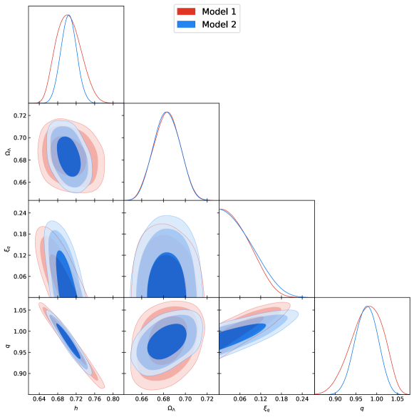
Figure 2: Confidence regions and PDFs for the parameters $h$, $\Omega_{\Lambda}$, $\xi_{q}$ and $q$, for the Model 1(blue) and Model 2(red) using tests with SN Ia + BAO + CMB.

Table 3: BAO distance measurements for each survey considered.

Survey	$z$	$d_{z}(z)$	Ref.
6dFGS	$0.106$	$0.3360\pm 0.0150$	bao1
MGS	$0.15$	$0.2239\pm 0.0084$	bao2
BOSS LOWZ	$0.32$	$0.1181\pm 0.0024$	bao4
SDSS(R)	$0.35$	$0.1126\pm 0.0022$	bao3
BOSS CMASS	$0.57$	$0.0726\pm 0.0007$	bao4

For each survey considered in the Table 3, the chi-squared function is given by

$$\chi_{\text{Survey}}^{2}=\left[\frac{d_{z}^{\,\text{obs}}(z)-d_{z}^{\,\text{mod}}(z)}{\sigma_{\text{Survey}}}\right]^{2},$$ (39)

where $d_{z}^{\,\text{obs}}$ is the observed ratio value, $d_{z}^{\,\text{mod}}$ is theoretical ratio value and $\sigma$ is the uncertainties in the measurements for each data point. And, for the WiggleZ data, the chi-squared function is

$$\chi_{\text{WiggleZ}}^{2}=\textbf{D}^{T}\textbf{C}^{-1}\textbf{D},$$ (40)

where $\textbf{D}=\mathbf{d}_{z}^{\,\text{obs}}-\mathbf{d}_{z}^{\,\text{mod}}$ and $\textbf{C}^{-1}$ is the covariance matrix given by Eq. (38).

Then, the BAO $\chi^{2}$ function contribution is defined as

$$\chi_{\text{BAO}}^{2}=\chi_{\text{Survey}}^{2}+\chi_{\text{WiggleZ}}^{2}$$ (41)

IV.3 CMB Data

In order to reduce the volume of the parameter space, we use the angular scale of the sound horizon at the last scattering, defined by

$$\ell_{a}=\pi\frac{r(z_{*})}{r_{s}(z_{*})},$$ (42)

where $r(z_{*})$ is the comoving distance of last scattering calculated in the redshift of the photon-decoupling surface, $z_{*}=1089.9$ planck

$$r(z_{*})=\frac{c}{H_{0}}\int_{0}^{z_{*}}\frac{dz}{E(z)},$$ (43)

and $r_{s}(z_{*})$ is the comoving sound horizon at last scattering. We use to constraint angular scale of the sound horizon at the last scattering data from Planck’s 2015, $\ell_{a}=301.63\pm 0.15$ planck . The angular scale of the sound horizon at the last scattering contribution to the total $\chi^{2}$ is

$$\chi^{2}_{CMB}=\frac{(\ell_{a}^{\text{obs}}-\ell_{a}^{\text{mod}})^{2}}{\sigma_{\ell_{a}}^{2}}.$$ (44)

Therefore, the function

$$\chi^{2}=\chi^{2}_{\text{Pan}}+\chi^{2}_{\text{BAO}}+\chi^{2}_{\text{CMB}},$$ (45)

which takes into account all the data sets mentioned above, should be minimized.

V Results and Conclusions

Table 4: Confidence limits for the cosmological parameters using the SN Ia, BAO, CMB data. The first column shows the constrains on the reference ${\Lambda}$CDM model whereas the second and third columns show the results for the Model 1 and for the Model 2.

Parameter	${\Lambda}$CDM	Model 1	Model 2
$h$	$0.693^{+0.012+0.024+0.031}_{-0.012-0.024-0.032}$	$0.704^{+0.024+0.051+0.066}_{-0.029-0.047-0.057}$	$0.704^{+0.017+0.034+0.043}_{-0.017-0.033-0.042}$
$\Omega_{dm}$	$0.249^{+0.012+0.024+0.032}_{-0.012-0.022-0.028}$	$-$	$-$
$\Omega_{\Lambda}$	$0.683^{+0.013+0.025+0.031}_{-0.013-0.025-0.031}$	$0.683^{+0.012+0.023+0.027}_{-0.012-0.023-0.028}$	$0.683^{+0.012+0.022+0.028}_{-0.012-0.022-0.027}$
$\xi_{q}$	$-$	$0.004^{+0.074+0.14+0.16}_{-0.074-0.15-0.16}$	$-0.003^{+0.085+0.16+0.19}_{-0.085-0.16-0.19}$
$q$	$-$	$0.977^{+0.043+0.069+0.082}_{-0.034-0.075-0.098}$	$0.975^{+0.027+0.052+0.062}_{-0.027-0.054-0.068}$
$\ln\mathcal{E}$	$-529.177\pm 0.010$	$-529.997\pm 0.042$	$-529.745\pm 0.017$
$\ln B$	$-$	$-0.820\pm 0.042$	$-0.568\pm 0.017$
Interpretation	$-$	Inconclusive	Inconclusive
$\xi_{q0}$	$-$	$6.0\times 10^{6}(2\sigma)$	$6.8\times 10^{6}(2\sigma)$

We perform a Bayesian analysis of the nonextensive viscous models considering the evidence according to Jeffreys’s scale Table 1. In this study we consider the priors shown in Table 2 and background data such as, type Ia supernova, baryon acoustic oscillations and angular scale of the sound horizon at the last scattering. We consider the physical constraint $\xi_{q}>0$ upon both models in order to guarantee that second law of thermodynamics should not be violated 3 ; 4 .

The main results of the analysis are shown in Table 4, where we present the joint analysis SN Ia + BAO + CMB with 68%, 95% and 99% confidence levels (CL). In the Fig. 2 show the confidence regions in $1\sigma$, $2\sigma$ and $3\sigma$ and the posterior distributions. Note that the results for both models are compatible with the $\Lambda$CDM predictions ($q=1.00$ and $\xi_{q}=0.0$) at $1\sigma$ and with the results published by Refs. 30 ; 16 ; 28 . We remark that values of models parameters are slightly similar for the two models. For model 2 we have at $1\sigma$ limit $\xi_{q}<0$, which violates the second law of thermodynamics. The extended $\Lambda$CDM model was able to fit the cosmological data at both $2\sigma$ and $3\sigma$ scenarios as well as recovered the standard $\Lambda$CDM model at $1\sigma$. The results obtained by our analysis constraint the value of Hubble constant, therefore we can calculate the discrepancy (or tension) between these values and Hubble constant local value riess2 . For Model 1, the tension is $1.078\sigma$ and for the Model 2, $1.329\sigma$, therefore the extended $\Lambda$CDM model alleviates the $H_{0}$ tension.

For the sake of comparison, we calculate Bayes’ factor considering $\Lambda$CDM as the reference model. In Table 4, we show the values obtained for the logarithm of the Bayesian evidence ($\ln\mathcal{E}$), logarithm of the Bayes factor ($\ln\mathcal{B}$) and interpretation of evidence for each model considering the data. We note that extended models are disfavored with inconclusive evidence with respect to the $\Lambda$CDM model.

For the models, the calculation of the nonextensive bulk viscosity parameter considering the $2\sigma$ value provides $\xi_{q}\sim 0.14$ (Model 1) and $\xi_{q}\sim 0.16$ (Model 2) or $\xi_{q0}\sim 10^{6}Pa.s$ in SI unity. This results are in agreement from the one calculated in the Refs. 44 ; 45 in which have used the standard interpretation for bulk viscosity.

To summarize, the cosmological observations are compatible with the extended model proposed through the constraints over $h$, $\Omega_{\Lambda}$, $\xi_{q}$ and $q$. In particular, the extensive limit $q=1$, the standard $\Lambda$CDM model is recovered.

It is worth emphasizing that the microscopic nonextensive approach can be used to describe the dark energy in the context of the bulk viscosity VDE . Furthermore, this description can be tested through the cosmography 61 and the quintessence scenarios 62 . These issues will appear in a forthcoming communication.

- (1) S. Weinberg, Rev. Mod. Phys. 61, 1 (1989); V. Sahni and A. A. Starobinsky, Int. J. Mod. Phys. D 9, 373 (2000), astro-ph/9904398; T. Padmanabhan, Phys. Rept. 380, 235 (2003), hepth/0212290.
- (2) E. Macaulay, I. K. Wehus, and H. K. Eriksen, Phys. Rev. Lett. 111, 161301 (2013), 1303.6583; W. L. Freedman, Nat. Astron. 1, 0169 (2017), 1706.02739; A. Amon et al. (2017), 1711.10999.
- (3) S. Capozziello, Int. J. Mod. Phys. D 11, 483 (2002), grqc/0201033.
- (4) E. J. Copeland, M. Sami, and S. Tsujikawa, Int. J. Mod. Phys. D 15, 1753 (2006), hep-th/0603057.
- (5) W. C. Algoner, H. E. S. Velten, and W. Zimdahl, JCAP 11, 034 (2016), grqc/1607.03952
- (6) M. Gell-Mann, C. Tsallis (Eds.), Nonextensive Entropy: Interdisciplinary Applications, Oxford University Press, New York, (2004).
- (7) N. Komatsu, S. Kimura, Phys. Rev. D 88, 083534 (2013); N. Komatsu, S. Kimura, Phys. Rev. D 89, 123501 (2014).
- (8) H. P. Oliveira, I.D. Soares, Phys. Rev. D 71, 124034 (2005).
- (9) T. S. Biro, V. G. Czinner, Phys. Lett. B 726, 861 (2013).
- (10) R. C. Nunes, et al. JCAP 08, 051 (2016); E. M. Barboza Jr., R. C. Nunes, E. M. C. Abreu, J. Ananias Neto, Physica A 436, 301 (2015); E. M. C. Abreu, J. Ananias Neto, A. C .R. Mendes, W. Oliveira, Physica A 392, 5154 (2013).
- (11) T. Osada, and G. Wilk, Phys. Rev. C 77, 044903 (2008); Phys. Rev. C 78, 069903 (2008); Erratum Phys. Rev. C 78, 069903 (2008).
- (12) T. Osada, G. Wilk, Indian J. Phys 85, 941 (2011).
- (13) H. S. Gimenes, G. M. Viswanathan, R. Silva, Physica A 494, 331 (2018).
- (14) R. Silva and J. A. S. Lima, Phys. Rev. E 72, 057101 (2005).
- (15) Z. B .B. de Oliveira and R. Silva, Ann. of Physics 375, 227 (2016); A. P. Santos, R. Silva, J. S. Alcaniz, J. A. S. Lima, Ann. Physics 386, 158 (2017).
- (16) C. Eckart, Phys. Rev. D 58, 919 (1940).
- (17) S. Weinberg, Gravitation and Cosmology (Wiley, New York, 1972).
- (18) S. Weinberg, Mod. Astrophys. J. 168, 175 (1971).
- (19) R. Treciokas and G. F. R. Ellis, Commun. Math. Phys. 23, 1 (1971).
- (20) M. Heller, Z. Klimek, and L. Suszycki, Astrophys. Space Sci. 20, 205 (1973).
- (21) G. L. Murphy Phys. Rev. D, 8, 4231 (1973).
- (22) Ya. B. Zeldovich, Sov. Phys. JETP Lett. 12, 307 (1970); G. L. Murphy, Phys. Rev. D 8, 4231 (1973); B. L. Hu, Phys. Lett. A 90, 375 (1982); J. A. S. Lima and A. S. M. Germano, Phys. Lett. A 170, 373 (1992); T. Harko, Phys. Rev. D 90, 044067 (2014).
- (23) J. A. S. Lima, J. F. Jesus, F. A. Oliveira, J. Cosmol. Astropart. Phys. 1011, 027 (2010); S. Basilakos, J. A. S. Lima, Phys. Rev. D 82, 023504 (2010); J. F. Jesus, F. A. Oliveira, S. Basilakos, J. A. S. Lima, Phys. Rev. D 84, 063511 (2011).
- (24) W. Zimdahl, D.J. Schwarz, A.B. Balakin, and D. Pavon, Phys. Rev. D 64, 063501 (2001).
- (25) A.B. Balakin, D. Pavon, D.J. Schwarz, and W. Zimdahl, New J. Phys. 5, 85 (2003).
- (26) R. Colistete Jr., J.C. Fabris, J. Tossa, and W. Zimdahl Phys. Rev. D 76, 103516 (2007).
- (27) A. Avelino and U. Nucamendi, JCAP 4, 006 (2009).
- (28) W.S. Hipolito-Ricaldi, H.E.S. Velten, and W. Zimdahl, JCAP 6, 016 (2009).
- (29) W.S. Hipolito-Ricaldi, H.E.S. Velten, and W. Zimdahl, Phys. Rev. D 82, 063507 (2010).
- (30) J.-S. Gagnon and J. Lesgourgues, JCAP 9, 026 (2011).
- (31) B. Li and J.D. Barrow, Phys. Rev. D 79, 103521 (2009).
- (32) H. Velten and D.J. Schwarz, JCAP 9, 016 (2011).
- (33) I. Brevik and O. Gron, in Recent Advances in Cosmology, (Eds). A. Travena and B. Soren, Nova Science Publishers (2013).
- (34) H. Velten, J. Wang, and X. Meng, Phys. Rev. D 88, 123504 (2013).
- (35) M. Cruz, S. Lepe, S. D. Odintsov arXiv:1808.03825[gr-qc](2018); F. Contreras, N. Cruz, E. Elizalde, E. González, S. Odintsov arXiv:1808.06546[gr-qc](2018); S. Nojiri, S. D. Odintsov, Phys.Rev. D 72 023003 (2005); S. Capozziello, V. F. Cardone, E. Elizalde, S. Nojiri, and S. D. Odintsov Phys. Rev. D 73, 043512 (2006); I. Brevik, et al. Int. J. Mod. Phys. D 26 (2017); I. Brevik, E. Elizalde, S. Nojiri, and S. D. Odintsov Phys. Rev. D 84, 103508 (2011); S. Anand, P. Chaubal, A. Mazumdar and S. Mohanty, JCAP 11, 005 (2017).
- (36) E. Verlinde, JHEP 1104 029 (2011); See also T. Padmanabhan, Mod. Phys. Lett. A, vol. 25, no. 14 1129 (2010).
- (37) W. G. Unruh, Phys. Rev. D 14, 870 (1976).
- (38) R.-G. Cai, L.-M. Cao, N. Ohta, Phys. Rev. D 81, 084012 (2010).
- (39) A. R. Plastino and J. A. S. Lima, Phys. Lett. A 260, 46 (1999).
- (40) R. Silva, A. R. Plastino and J. A. S. Lima, Phys. Lett. A 249, 401 (1998).
- (41) A. Lavagno, Phys. Lett. A 301, 13 (2002).
- (42) B. Santos, N. C. Devi, and J. S. Alcaniz, Phys. Rev. D 95, 123514 (2017).
- (43) M. A. Santos, M. Benetti, J. Alcaniz, F. A. Brito, and R. Silva, JCAP 1803, 023 (2018).
- (44) S. Santos da Costa, M. Benetti, and J. Alcaniz, JCAP 1803, 004 (2018).
- (45) U. Andrade, C. A. P. Bengaly, J. S. Alcaniz, B. Santos, Phys. Rev. D 97, 083518 (2018).
- (46) A. Cid, B. Santos, C. Pigozzo, T. Ferreira, J. Alcaniz, arXiv:1805.02107[astro-ph.CO].
- (47) R. Trotta, Contemp. Phys. 49, 71 (2008), arXiv:0803.4089[astro-ph].
- (48) H. Jeffreys, Theory of Probability, 3rd ed. (Oxford Univ. Press, Oxford, England, 1961).
- (49) J. Buchner et. al., Astronomy & Astrophysics, 564, A125 (2014). https://github.com/JohannesBuchner/PyMultiNest.
- (50) F. Feroz and M. P. Hobson, Mon. Not. Roy. Astron. Soc. 384, 449 (2008).
- (51) F. Feroz, M. P. Hobson, and M. Bridges, Mon. Not. Roy. Astron. Soc. 398, 1601 (2009).
- (52) F. Feroz, M. P. Hobson, E. Cameron, and A. N. Pettitt, ArXiv e-prints (2013), arXiv:1306.2144[astro-ph.IM].
- (53) J. Skilling, AIP Conf. Proc. 735, 395 (2004).
- (54) A. Lewis and S. Bridle, “GetDist.”. https://cosmologist.info/cosmomc/readme.html. Accessed July 2018.
- (55) A. G. Riess et al., Astrophys. J. 826, 56 (2016).
- (56) D. M. Scolnic et al, The Astrophysical Journal, 859, 2 (2018).
- (57) M. Betoule et al., Astronomy & Astrophysics 568, A22 (2014).
- (58) A. Conley et al. The Astrophysical Journal Supplement Series 192, 1 (2010).
- (59) D. J. Eisenstein et al. (SDSS Collaboration), The Astrophysical Journal, 633, 2 (2005).
- (60) D. J. Eisenstein and W. Hu, The Astrophysical Journal, 496, 605 (1998).
- (61) C. Blake et al., Mon. Not. R. Astron. Soc. 425, 405 (2012).
- (62) F. Beutler, C. Blake, M. Colless, D. H. Jones, L. Staveley-Smith, L. Campbell, Q. Parker, W. Saunders, and F. Watson, Mon. Not. R. Astron. Soc. 416, 3017 (2011).
- (63) A. J. Ross, L. Samushia, C. Howlett, W. J. Percival, A. Burden, and M. Manera, Mon. Not. R. Astron. Soc. 449, 835 (2015).
- (64) L. Anderson et al. (BOSS), Mon. Not. R. Astron. Soc. 441, 24 (2014).
- (65) N. Padmanabhan, X. Xu, D. J. Eisenstein, R. Scalzo, A. J. Cuesta, K. T. Mehta, and E. Kazin, Mon. Not. R. Astron. Soc. 427, 2132 (2012).
- (66) P. A. R. Ade et al. (Planck Collaboration), Astron. Astrophys. 594, A13 (2016); P. A. R. Ade et al. (Planck Collaboration) Astron. Astrophys. 594, A14 (2016).
- (67) M. Vargas dos Santos, R. R. R. Reis and I. Waga J. Cosmol. Astropart. Phys. 02, 66 (2016).
- (68) A. G. Riess et al., The Astrophysical Journal, 861, 2 (2018) arXiv:1804.10655.
- (69) H. Velten, D. J. Schwarz, Phys. Rev. D 86 083501 (2012).
- (70) I. Brevik, O. Gorbunova, Gen. Relativity Gravitation 37, 2039 (2005); I. Brevik, Entropy 17, 6318 (2015); J. Wang, X. Meng, Modern Phys. Lett. A 29 1450009 (2014); B. D. Normann, I. Brevik, Entropy 18, 215 (2016); B. D. Normann, I. Brevik, Modern Phys. Lett. A 32, 1750026 (2017).
- (71) Wang, D., Yan, YJ. and Meng, XH. Eur. Phys. J. C 77, 660 (2017); B. Mostaghel, H. Moshafi and S. M. S. Movahed, Eur. Phys. J. C 77, 541 (2017).
- (72) K. Bamba, S. Capozziello, S. Nojiri, S. D. Odintsov, Astrophys. Space Sci. 342, 155 (2012).
- (73) H. H. B. Silva, R. Silva, R. S. Gonçalves, Zong-Hong Zhu, and J. S. Alcaniz, Phys. Rev. D 88, 127302 (2013).