Weak decays of the axial-vector tetraquark $T_{bb;\bar{u}\bar{d}}^{-}$

Abstract

The weak decays of the axial-vector tetraquark $T_{bb;\bar{u}\bar{d}}^{-}$ to the scalar state $Z_{bc;\bar{u}\bar{d}}^{0}$ are investigated using the QCD three-point sum rule approach. In order to explore the process $T_{bb;\bar{u}\bar{d}}^{-}\to Z_{bc;\bar{u}\bar{d}}^{0}l\bar{\nu_{l}}$, we recalculate the spectroscopic parameters of the tetraquark $T_{bb;\bar{u}\bar{d}}^{-}$ and find the mass and coupling of the scalar four-quark system $Z_{bc;\bar{u}\bar{d}}^{0}$, which are important ingredients of calculations. The spectroscopic parameters of these tetraquarks are computed in the framework of the QCD two-point sum rule method by taking into account various condensates up to dimension ten. The mass of the $T_{bb;\bar{u}\bar{d}}^{-}$ state is found to be $m=(10035~{}\pm 260)~{}\mathrm{MeV}$, which demonstrates that it is stable against the strong and electromagnetic decays. The full width $\Gamma$ and mean lifetime $\tau$ of $T_{bb;\bar{u}\bar{d}}^{-}$ are evaluated using its semileptonic decay channels $T_{bb;\bar{u}\bar{d}}^{-}\to Z_{bc;\bar{u}\bar{d}}^{0}l\bar{\nu_{l}}$, $l=e,\mu$ and $\tau$. The obtained results, $\Gamma=(7.17\pm 1.23)\times 10^{-8\ \ }\mathrm{MeV}$ and $\tau=9.18_{-1.34}^{+1.90}~{}\mathrm{fs}$, can be useful for experimental investigations of the doubly-heavy tetraquarks.

I Introduction

Assumptions about the existence of four-quark bound states (tetraquarks) were made in an early stage of QCD and aimed to explain some of the unusual features of meson spectroscopy. Thus, the nonet of light scalar mesons was considered as bound states of four light quarks rather than being composed of a quark and an antiquark, as in the standard models of the mesons. The stability problems of heavy and heavy-light tetraquarks were also among the questions addressed in these studies Jaffe:1976ig ; Jaffe:1976ih ; Weinstein:1982gc ; Ader:1981db .

Due to the impressive experimental discoveries and theoretical progress of the past $15$ years the study of multiquark hadrons has become an integral part of high energy physics. During this period of development and growth various difficulties in experimental studies, and the classification and theoretical interpretation of numerous tetraquarks were successfully overcome Chen:2016qju ; Esposito:2016noz ; Ali:2017jda ; Olsen:2017bmm .

But there are still problems in the physics of exotic hadrons that are not fully solved; the identification of the tetraquark resonances and their stability are among these questions. It is known that the first charmonium-like resonances observed experimentally were interpreted not only as tetraquarks, but also as excited states of the conventional charmonium. Fortunately, there are different classes of tetraquarks that cannot be identified as charmonia or bottomonia states. Indeed, charged resonances carrying one or two units of electric charge and states containing two or more open quark flavors can easily be distinguished from charmonium- or bottomonium-like structures. All of the resonances observed in various experiments and classified as tetraquarks are unstable with respect to strong interactions. They lie either above the open charm (-bottom) thresholds or are very close to them. Such four-quark compounds can strongly decay to two conventional mesons. Because quarks required to create these mesons already exist in the master particles, the width of such states is rather large: the dissociation into two mesons is the main strong decay channel of the unstable tetraquarks.

It is natural that theoretical explorations of stable four-quark systems and their experimental discovery remain on the agenda of particle physics. The tetraquarks built of heavy $cc$ or $bb$ diquarks and light antidiquarks are real candidates for such states. Their studies have a long history; in fact, the class of exotic mesons $QQ\bar{Q}\bar{Q}$ and $QQ\bar{q}\bar{q}$ were studied in Refs. Ader:1981db ; Lipkin:1986dw ; Zouzou:1986qh , where a potential model with an additive pairwise interaction was used to search for stable tetraquarks. It was demonstrated that in the context of this approach the exotic mesons composed of only heavy quarks are unstable, but the tetraquarks $QQ\bar{q}\bar{q}$ may form stable compounds provided the ratio $m_{Q}/m_{q}$ is large. The same conclusions were made in Ref. Carlson:1987hh , in which the only constraint imposed on the confining potential was its finiteness when two particles come close together. There it was found that the isoscalar $J^{P}=1^{+}$ tetraquark $T_{bb;\bar{u}\bar{d}}^{-}$ resides below the two-B-meson threshold, and hence can decay only weakly. At the same time, the tetraquarks $T_{cc;\bar{q}\bar{q}^{\prime}}$ and $T_{bc;\bar{q}\bar{q}^{\prime}}$ may exist as unstable or stable bound states. The stability of the $QQ\overline{q}\overline{q}$ compounds in the limit $m_{Q}\rightarrow\infty$ was studied in Ref. Manohar:1992nd , as well.

Various theoretical models-starting from the chiral and dynamical quark models and ending with the relativistic quark model-were used to study the properties and compute the masses of the $T_{QQ}$ states Pepin:1996id ; Janc:2004qn ; Cui:2006mp ; Vijande:2006jf ; Ebert:2007rn . The masses of the axial-vector states $T_{QQ;\bar{u}\bar{d}}$ were also extracted from the two-point sum rules Navarra:2007yw . In accordance with the results of Ref. Navarra:2007yw , the mass of the tetraquark $T_{bb;\bar{u}\bar{d}}^{-}$ is $10.2\pm 0.3\ \mathrm{GeV}$, which is below the open-bottom threshold. Using the same method, the parameters of the $QQ\bar{q}\bar{q}$ states with the spin-parities $0^{-},\ 0^{+},\ 1^{-}$ and $1^{+}$ were evaluated in Ref. Du:2012wp . The production mechanisms of the $T_{cc}$ tetraquarks-such as the heavy ion and proton-proton collisions, electron-positron annihilations, $B_{c}$ meson and heavy $\Xi_{bc\text{ }}$ baryon decays-as well as possible decay channels of the $T_{cc}$ states were addressed in the literature SchaffnerBielich:1998ci ; DelFabbro:2004ta ; Lee:2007tn ; Hyodo:2012pm ; Esposito:2013fma .

The discovery of the doubly charmed baryon $\Xi_{cc}^{++}=ccu$ by the LHCb Collaboration Aaij:2017ueg inspired new investigations of double-charm, double-bottom and four-bottom tetraquarks Karliner:2017qjm ; Luo:2017eub ; Eichten:2017ffp ; Wang:2017dtg ; Ali:2018ifm ; Ali:2018xfq ; Eichten:2017ual ; Hughes:2017xie ; Esposito:2018cwh . Lattice simulations in the context of nonrelativistic QCD to search for the existence of the bound states $T_{bb;\overline{b}\overline{b}}^{0}$ below the lowest bottomonium-pair threshold were carried out in Ref. Hughes:2017xie , but no evidence was found for such stable states with quantum numbers $0^{++},\ 1^{+-}$ and $2^{++}$, which can be considered a present-day confirmation of the conclusions originally made in Refs. Ader:1981db ; Lipkin:1986dw ; Zouzou:1986qh ; Carlson:1987hh . A situation with double-bottom tetraquarks is more promising. Thus, the mass of the state $T_{bb;\overline{u}\overline{d}}^{-}$ was estimated once more in the framework of a phenomenological model in Ref. Karliner:2017qjm . There, the mass of the isoscalar axial-vector state $T_{bb;\overline{u}\overline{d}}^{-}$ was found to be $m=10389\pm 12\ \mathrm{MeV}$ which is $215\ \mathrm{MeV}$ below the $B^{-}\overline{B}^{\ast 0}$ threshold and $170\ \mathrm{MeV}$ below the threshold for $B^{-}\overline{B}^{0}\gamma$ decay. This means that the tetraquark $T_{bb;\overline{u}\overline{d}}^{-}$ is stable against the strong and electromagnetic decays and only decays weakly. At the same time, the mass of the double-charm $T_{cc;\overline{u}\overline{d}}^{+}$ state is $3882\pm 12\ \mathrm{MeV}$, which is above the thresholds of both $D^{0}D^{\ast+}$ and $D^{0}D^{+}\gamma$ decays (see Ref.  Karliner:2017qjm ). The double-charm states $T_{cc;\overline{s}\overline{s}}^{++}$ and $T_{cc;\overline{d}\overline{s}}^{++}$ that belong to the class of doubly charged tetraquarks were investigated recently in our work Agaev:2018vag . These particles carry two units of electric charge, which makes them particularly interesting. They are above the $D_{s}^{+}D_{s0}^{\ast+}(2317)$ and $D^{+}D_{s0}^{\ast+}(2317)$ thresholds, and the width of the strong decays $T_{cc;\overline{s}\overline{s}}^{++}\rightarrow D_{s}^{+}D_{s0}^{\ast+}(2317)$ and $T_{cc;\overline{d}\overline{s}}^{++}\rightarrow D^{+}D_{s0}^{\ast+}(2317)$ allowed us to classify them as relatively broad resonances.

In light of recent progress made in the physics of double-heavy tetraquarks and the expected stability of the $T_{bb;\overline{u}\overline{d}}^{-}$ state, its weak decays are a very interesting subject for a detailed analysis. The semileptonic decays of four-quark systems- when an initial tetraquark transforms into a final tetraquark and $l\overline{\nu}_{l}$ or $\overline{l}\nu_{l}$ leptons- are a relatively new topic in the physics of exotic mesons Sundu:2018uyi ; Xing:2018bqt . In Ref. Sundu:2018uyi the decay of the axial-vector tetraquark $Z_{s}=[cs][\overline{b}\overline{s}]$ to a final state $X(4274)\overline{l}\nu_{l}$ was studied using the QCD sum rule method. The widths of these decays, (where $l=e,\mu$ and $\tau$) are very small, and therefore the transitions $Z_{s}\rightarrow X(4274)\overline{l}\nu_{l}\$ were classified as rare processes. The semileptonic decays of the stable double heavy tetraquarks were considered in Ref. Xing:2018bqt .

In the present work we are going to explore the semileptonic decays of the tetraquark $T_{bb;\overline{u}\overline{d}}^{-}$ and evaluate its full width and mean lifetime. The tetraquark $T_{bb;\overline{u}\overline{d}}^{-}$ undergoes weak decay through the transition $b\rightarrow W^{-}c$. In the final state, its decay products consist of $l\overline{\nu}_{l}$ and a diquark-antidiquark $Z_{bc;\bar{u}\bar{d}}^{0}=[bc][\overline{u}\overline{d}]$ state (for simplicity, hereafter $Z_{bc}^{0}$). The tetraquark $Z_{bc}^{0}$ may decay to $B$ and $D$ mesons with appropriate masses and spin-parities provided its mass is larger than corresponding thresholds. In this scenario $Z_{bc}^{0}$ dissociates strongly to the final conventional mesons. Otherwise, at the next stage $Z_{bc}^{0}$ should decay due to weak or electromagnetic interactions. In the present work we restrict ourselves by considering the semileptonic decay of $T_{bb;\overline{u}\overline{d}}^{-}$ only to the scalar state $Z_{bc}^{0}$.

The open charm-bottom four-quark systems $QQ^{\prime}\bar{q}\bar{q}$ were already analyzed in Refs. Zouzou:1986qh ; SilvestreBrac:1993ry . In recent investigations these compounds were treated either as $B_{c}$-like molecular or $Z_{bc}=[bc][\overline{q}\overline{q}]$-type diquark-antidiquark states. The masses of the $B_{c}$-like scalar and axial-vector molecules with different light-quark contents and spin-parities were calculated in Refs.Sun:2012sy ; Albuquerque:2012rq . The open charm-bottom states were analyzed in Ref. Chen:2013aba in the framework of the diquark-antidiquark model. In order to extract the masses of these states, the authors utilized the QCD sum rule method and interpolating currents of different color structure. The class of open charm-bottom tetraquarks also includes states with $(b,\overline{c})$ or $(c,\overline{b})$ quarks which were the subject of rather intensive studies as well Sun:2012sy ; Albuquerque:2012rq ; Chen:2013aba ; Zhang:2009vs ; Zhang:2009em ; Agaev:2016dsg ; Agaev:2017uky . In fact, the molecule-type tetraquarks with the contents $\{Q\overline{q}\}\{\overline{Q}^{(\prime)}q\}$ and $\{Q\overline{s}\}\{\overline{Q}^{(\prime)}s\}$ were studied in Refs. Zhang:2009vs and Zhang:2009em , respectively. In these papers the masses of these hypothetical particles were computed in the context of the QCD two-point sum rule approach using vacuum condensates up to dimension six. The spectroscopic parameters and strong decays of the scalar and axial-vector tetraquarks $Z_{q}=[cq][\overline{b}\overline{q}]$ and $Z_{s}=[cs][\overline{b}\overline{s}]$ were calculated in Refs. Agaev:2016dsg and Agaev:2017uky , respectively.

It is remarkable that $Z_{bc}^{0}=[bc][\overline{u}\overline{d}]$ is the open charm-bottom tetraquark, and that it contains four quarks of different flavors. Two years ago, data on the state known as $X(5568)$ from the D0 Collaboration D0:2016mwd led to an interest in compound systems of four distinct quarks. However, both the experimental and theoretical studies of $X(5568)$ led to controversial conclusions, leaving the status of this tetraquark unclear. Therefore investigating the process $T_{bb;\overline{u}\overline{d}}^{-}\rightarrow Z_{bc}^{0}l\overline{\nu}_{l}$ could not only help to answer questions about features of the tetraquark $T_{bb;\overline{u}\overline{d}}^{-}$ itself, but also to clarify the structure and properties of its decay products.

The spectroscopic parameters of $T_{bb;\overline{u}\overline{d}}^{-}$ and $Z_{bc}^{0}$ are important input for studying the semileptonic decay under consideration. In the present work, we calculate the masses and couplings of these tetraquarks by employing QCD sum rules obtained from an analysis of the relevant two-point correlation functions. When computing the correlation functions, we take into account the vacuum expectation values of the quark, gluon, and mixed local operators up to dimension ten. We evaluate the width of the semileptonic decay $T_{bb;\overline{u}\overline{d}}^{-}\rightarrow Z_{bc}^{0}l\overline{\nu}_{l}$ by applying the standard prescriptions of the QCD three-point sum rule method. Our aim here is to extract the sum rules for the weak form factors $G_{i}(q^{2}),\,i=0,1,2,3$ and to compute their numerical values. This allows us to determine the so-called fit functions $F_{i}(q^{2})$, which coincide with $G_{i}(q^{2})$, but can be extended to a region of momentum transfers that is not accessible to the QCD sum rules. The functions $F_{i}(q^{2})$ are used to integrate the differential decay rate $d\Gamma/dq^{2}$ and find the partial width of the decay processes $\Gamma\left(T_{bb;\overline{u}\overline{d}}^{-}\rightarrow Z_{bc}^{0}l\overline{\nu}_{l}\right)$, $l=e,\ \mu$ and $\tau$.

This article is organized in the following manner: In Sec. II we derive the QCD two-point sum rules for the masses and couplings of the tetraquarks $T_{bb;\overline{u}\overline{d}}^{-}$ and $Z_{bc}^{0}$, and numerically compute their values. In Sec.III we use the QCD three-point correlation function to derive sum rules for the weak form factors $G_{i}(q^{2})$. In this section we also perform a numerical analysis of the obtained sum rules and determine the fit functions, which allow us to evaluate the width of the semileptonic decay $T_{bb;\overline{u}\overline{d}}^{-}\rightarrow Z_{bc}^{0}l\overline{\nu}_{l}$ and mean lifetime of the state $T_{bb;\overline{u}\overline{d}}^{-}$. Section IV contains a discussion of the obtained results and our brief conclusions. The explicit expression for the decay rate $d\Gamma/dq^{2}$ can be found in the Appendix.

II Spectroscopic parameters of the tetraquarks $T_{bb;\overline{u}\overline{d}}^{-}$ and $Z_{bc}^{0}$

In this section we calculate the spectroscopic parameters of the tetraquarks $T_{bb;\overline{u}\overline{d}}^{-}$ and $Z_{bc}^{0}$ by employing the QCD two-point sum rules extracted from analysis of the relevant correlation functions $\Pi_{\mu\nu}(p)$ and $\Pi(p)$. The masses of $T_{bb;\overline{u}\overline{d}}^{-}$ and $Z_{bc}$ in the framework of QCD sum rules were found in Refs. Navarra:2007yw ; Du:2012wp and Chen:2013aba , respectively. We are going to evaluate the masses and tetraquark-current couplings of these states by taking into account the vacuum condensates up to dimension ten which exceeds the accuracy of the previous studies: updated information on the spectroscopic parameters of the tetraquarks $T_{bb;\overline{u}\overline{d}}^{-}$ and $Z_{bc}^{0}$ is necessary to explore the semileptonic decay $T_{bb;\overline{u}\overline{d}}^{-}\rightarrow Z_{bc}^{0}l\overline{\nu}_{l}$ in the next section.

The function $\Pi_{\mu\nu}(p)$ is defined as

$$\Pi_{\mu\nu}(p)=i\int d^{4}xe^{ip\cdot x}\langle 0|\mathcal{T}\{J_{\mu}(x)J_{\nu}^{{\dagger}}(0)\}|0\rangle,$$ (1)

where $J_{\mu}(x)$ is the interpolating current to the axial-vector tetraquark $T_{bb;\overline{u}\overline{d}}^{-}$ composed of an axial-vector diquark and a scalar antidiquark. This current is given by Navarra:2007yw

$$J_{\mu}(x)=b_{a}^{T}(x)C\gamma_{\mu}b_{b}(x)\overline{u}_{a}(x)\gamma_{5}C\overline{d}_{b}^{T}(x).$$ (2)

Here, $a$ and $b$ are the color indices and $C$ is the charge-conjugation operator.

The correlation function $\Pi(p)$ for the scalar tetraquark $Z_{bc}^{0}$ has the form

$$\Pi(p)=i\int d^{4}xe^{ip\cdot x}\langle 0|\mathcal{T}\{J^{Z}(x)J^{Z{\dagger}}(0)\}|0\rangle,$$ (3)

where the current $J^{Z}(x)$ is defined as

$$J^{Z}(x) = b_{a}^{T}(x)C\gamma_{5}c_{b}(x)\left[\overline{u}_{a}(x)\gamma_{5}C\overline{d}_{b}^{T}(x)\right.$$ (4)

$$\left.-\overline{u}_{b}(x)\gamma_{5}C\overline{d}_{a}^{T}(x)\right],$$

and is obtained using currents for the diquark-antidiquarks $Z_{bc}$ from Ref. Chen:2013aba . The current $J^{Z}(x)$ is composed of a scalar diquark and an antidiquark in the antitriplet and triplet representations of the color group, respectively.

Here we concentrate on calculating the parameters of the tetraquark $T_{bb;\overline{u}\overline{d}}^{-}$ and only provide necessary expressions and final results for $Z_{bc}^{0}$. In accordance with QCD sum rule method one first has to express the correlation function $\Pi_{\mu\nu}(p)$ in terms of the tetraquarks’ mass $m$ and coupling $f$, which form the phenomenological or physical side of the sum rules. We treat the tetraquark $T_{bb;\overline{u}\overline{d}}^{-}$ as a ground-state particle in its class, and therefore we isolate only the first term in $\Pi_{\mu\nu}^{\mathrm{Phys}}(p)$ which is given by

$$\Pi_{\mu\nu}^{\mathrm{Phys}}(p)=\frac{\langle 0|J_{\mu}|T(p)\rangle\langle T(p)|J_{\nu}^{\dagger}|0\rangle}{m^{2}-p^{2}}+\dots.$$ (5)

This expression is derived by saturating the correlation function (1) with a complete set of states with $J^{P}=1^{+}$ and performing the integration over $x$. The dots here indicate contributions to $\Pi_{\mu\nu}^{\mathrm{Phys}}(p)$ from higher resonances and continuum states.

The function $\Pi_{\mu\nu}^{\mathrm{Phys}}(p)$ can be further simplified by introducing the matrix element

$$\langle 0|J_{\mu}|T(p,\epsilon)\rangle=fm\epsilon_{\mu},$$ (6)

where $\epsilon_{\mu}$ is the polarization vector of the $T_{bb;\overline{u}\overline{d}}^{-}$ state. It is not difficult to demonstrate that in terms of $m$ and $f$ the function takes the following form

$$\Pi_{\mu\nu}^{\mathrm{Phys}}(p)=\frac{m^{2}f^{2}}{m^{2}-p^{2}}\left(-g_{\mu\nu}+\frac{p_{\mu}p_{\nu}}{m^{2}}\right)+\ldots$$ (7)

To suppress the contribution arising from the higher resonances and continuum, we carry out the Borel transformation of the correlation function, which reads

$$\mathcal{B}\Pi_{\mu\nu}^{\mathrm{Phys}}(p)=m^{2}f^{2}e^{-m^{2}/M^{2}}\left(-g_{\mu\nu}+\frac{p_{\mu}p_{\nu}}{m^{2}}\right)+\ldots,$$ (8)

where $M^{2}$ is the Borel parameter.

The second part of the sum rules is given by the same correlation function $\Pi_{\mu\nu}(p)$, but expressed in terms of the quark propagators

$$\Pi_{\mu\nu}^{\mathrm{OPE}}(p)=i\int d^{4}xe^{ip\cdot x}\left\{\mathrm{Tr}\left[\gamma_{5}\widetilde{S}_{d}^{b^{\prime}b}(-x)\gamma_{5}S_{u}^{a^{\prime}a}(-x)\right]\right.$$

$$\times\mathrm{Tr}\left[\gamma_{\nu}\widetilde{S}_{b}^{aa^{\prime}}(x)\gamma_{\mu}S_{b}^{bb^{\prime}}(x)\right]-\mathrm{Tr}\left[\gamma_{5}\widetilde{S}_{d}^{b^{\prime}b}(-x)\right.$$

$$\left.\left.\times\gamma_{5}S_{u}^{a^{\prime}a}(-x)\right]\mathrm{Tr}\left[\gamma_{\nu}\widetilde{S}_{b}^{ba^{\prime}}(x)\gamma_{\mu}S_{b}^{ab^{\prime}}(x)\right]\right\}.$$ (9)

In Eq. (9) $S_{b}^{ab}(x)$ and $S_{q}^{ab}(x)$ are the $b$ and $q(u,d)$-quark propagators, explicit expression for which can be found, for example, in Ref. Sundu:2018uyi . Here we also introduce the notation

$$\widetilde{S}_{b(q)}(x)=CS_{b(q)}^{T}(x)C.$$ (10)

The QCD sum rules can be extracted by using the same Lorentz structures in both $\Pi_{\mu\nu}^{\mathrm{Phys}}(p)$ and $\Pi_{\mu\nu}^{\mathrm{OPE}}(p)$. The structures $\sim g_{\mu\nu}$ are appropriate for our purposes, because they receive contributions only from spin-$1$ particles. The invariant amplitude $\Pi^{\mathrm{OPE}}(p^{2})$ corresponding to this structure can be represented by the dispersion integral

$$\Pi^{\mathrm{OPE}}(p^{2})=\int_{4m_{b}^{2}}^{\infty}\frac{\rho^{\mathrm{OPE}}(s)}{s-p^{2}}ds+\ldots,$$ (11)

where $\rho^{\mathrm{OPE}}(s)$ is the two-point spectral density. It is proportional to the imaginary part of the structure $\sim g_{\mu\nu}$ in the function $\Pi_{\mu\nu}^{\mathrm{OPE}}(p).$ In the present work, $\rho^{\mathrm{OPE}}(s)$ is calculated by taking into account the quark, gluon, and mixed vacuum condensates up to dimension ten.

By applying the Borel transformation to $\Pi^{\mathrm{OPE}}(p^{2})$, equating the obtained expression with the relevant part of the function $\mathcal{B}\Pi_{\mu\nu}^{\mathrm{Phys}}(p)$, and performing the continuum subtraction we find the final sum rules. Then, the mass of the $T_{bb\overline{u}\overline{d}}^{-}$ state can be evaluated from the sum rule

$$m^{2}=\frac{\int_{4m_{b}^{2}}^{s_{0}}dss\rho^{\mathrm{OPE}}(s)e^{-s/M^{2}}}{\int_{4m_{b}^{2}}^{s_{0}}ds\rho^{\mathrm{OPE}}(s)e^{-s/M^{2}}},$$ (12)

whereas to find the coupling $f$ we employ the expression

$$f^{2}=\frac{1}{m^{2}}\int_{4m_{b}^{2}}^{s_{0}}ds\rho^{\mathrm{OPE}}(s)e^{(m^{2}-s)/M^{2}}.$$ (13)

Here $s_{0}$ is the continuum threshold parameter that separates the ground-state and continuum contributions from one another.

In the case of the scalar tetraquark $Z_{bc}^{0}$, there are some differences stemming from its spin-parity and the structure of the interpolating current. Thus, the matrix element $\langle 0|J^{Z}|Z(p)\rangle$ has the form

$$\langle 0|J^{Z}|Z(p)\rangle=f_{Z}m_{Z},$$ (14)

which is analogous to the matrix element of a conventional scalar meson. The correlation function $\Pi^{\mathrm{OPE}}(p)$ is given by

$$\Pi^{\mathrm{OPE}}(p)=i\int d^{4}xe^{ip\cdot x}\mathrm{Tr}\left[S_{c}^{bb^{\prime}}(x)\gamma_{5}\widetilde{S}_{b}^{aa^{\prime}}(x)\gamma_{5}\right]$$

$$\times\left\{\mathrm{Tr}\left[\gamma_{5}\widetilde{S}_{d}^{b^{\prime}b}(-x)\gamma_{5}S_{u}^{a^{\prime}a}(-x)\right]-\mathrm{Tr}\left[\gamma_{5}\widetilde{S}_{d}^{a^{\prime}b}(-x)\right.\right.$$

$$\left.\times\gamma_{5}S_{u}^{b^{\prime}a}(-x)\right]-\mathrm{Tr}\left[\gamma_{5}\widetilde{S}_{d}^{b^{\prime}a}(-x)\gamma_{5}S_{u}^{a^{\prime}b}(-x)\right]$$

$$\left.+\mathrm{Tr}\left[\gamma_{5}\widetilde{S}_{d}^{a^{\prime}a}(-x)\gamma_{5}S_{u}^{b^{\prime}b}(-x)\right]\right\}.$$ (15)

The remaining manipulations and final sum rules for $m_{Z}$ and $f_{Z}$ are similar to those for the tetraquark $T_{bb;\overline{u}\overline{d}}^{-}$.

Parameters	Values
$m_{b}$	$4.18^{+0.04}_{-0.03}~{}\mathrm{GeV}$
$m_{c}$	$(1.27\pm 0.03)~{}\mathrm{GeV}$
$\langle\bar{q}q\rangle$	$-(0.24\pm 0.01)^{3}$ $\mathrm{GeV}^{3}$
$\langle\bar{s}s\rangle$	$0.8\ \langle\bar{q}q\rangle$
$m_{0}^{2}$	$(0.8\pm 0.1)$ $\mathrm{GeV}^{2}$
$\langle\overline{q}g_{s}\sigma Gq\rangle$	$m_{0}^{2}\langle\bar{q}q\rangle$
$\langle\overline{s}g_{s}\sigma Gs\rangle$	$m_{0}^{2}\langle\bar{s}s\rangle$
$\langle\frac{\alpha_{s}G^{2}}{\pi}\rangle$	$(0.012\pm 0.004)$ $~{}\mathrm{GeV}^{4}$
$\langle g_{s}^{3}G^{3}\rangle$	$(0.57\pm 0.29)$ $~{}\mathrm{GeV}^{6}$

Table 1: The parameters utilized in numerical computations.

The obtained sum rules depend on the quark, gluon, and mixed condensates, the numerical values of which are collected in Table 1. This table also contains the masses of the $b$ and $c$ quarks, which appear in the sum rules as input parameters.

Besides, Eqs. (12) and (13) depend on the auxiliary parameters $M^{2}$ and $s_{0}$, which should satisfy the standard constraints of the sum rule computations. Our analysis proves that the working windows

$$M^{2}\in[9,~{}13]\ \mathrm{GeV}^{2},\ s_{0}\in[115,~{}120]\ \mathrm{GeV}^{2}$$ (16)

meet all of the restrictions imposed on $M^{2}$ and $s_{0}$. Thus, the maximum of the Borel parameter is determined from the minimum allowed value of the pole contribution ($\mathrm{PC}$), which at $M^{2}=13~{}\mathrm{GeV}^{2}$ is $16\%$ of the full correlation function. Within the region $M^{2}\in[9,~{}13]~{}\mathrm{GeV}^{2}$ the pole contribution varies from $59$ to $16\%$. The lower limit of the Borel parameter is fixed by the convergence of the operator product expansion (OPE) for the correlation function. In the present work, we use the criterion

$$R(M^{2})=\frac{\Pi^{\mathrm{Dim(8+9+10)}}(M^{2},\ s_{0})}{\Pi(M^{2},\ s_{0})}<0.05,$$ (17)

where $\Pi(M^{2},\ s_{0})$ is the Borel-transformed and subtracted function $\Pi^{\mathrm{OPE}}(p^{2})$, and $\Pi^{\mathrm{Dim(8+9+10)}}(M^{2},\ s_{0})$ is the contribution from the last three terms in its expansion. At $M^{2}=9~{}\mathrm{GeV}^{2}$ the ratio $R$ is equal to $R(9~{}\mathrm{GeV}^{2})=0.01$, which ensures the excellent convergence of the sum rules. Moreover, at $M^{2}=9~{}\mathrm{GeV}^{2}$ the perturbative contribution amounts to $74\%$ of the full result, considerably exceeding the nonperturbative terms.

The quantities evaluated by means of the sum rules, in general, should not depend on the auxiliary parameters $M^{2}$ and $s_{0}$. But in calculations of the mass $m$ and coupling $f$ we observe a residual dependence on $M^{2}$ and $s_{0}$. Therefore, the stability of the extracted parameters (i.e., $m$ and $f$) is a necessary condition to fix the working windows for $M^{2}$ and $s_{0}$. In Figs. 1 and 2 we plot the dependence of the mass and coupling of the tetraquark $T_{bb;\overline{u}\overline{d}}^{-}$ on the parameters $M^{2}$ and $s_{0}$. It is seen that $m$ and $f$ depend on $M^{2}$ and $s_{0}$, which generates the main part of the theoretical errors inherent to the sum rule computations. For the mass $m$ these ambiguities are small, whereas for the coupling $f$ they may be sizable. This behavior has a simple explanation: the sum rule for the mass of the tetraquark (12) is given as the ratio of integrals over the functions $s\rho^{\mathrm{OPE}}(s)$ and $\rho^{\mathrm{OPE}}(s)$, which considerably reduces effects due to the variation of $M^{2}$ and $s_{0}$. The coupling $f$ depends on the integral over the spectral density $\rho^{\mathrm{OPE}}(s)$ itself, and therefore undergoes relatively sizable changes. In the case under discussion, theoretical errors for $m$ and $f$ stemming from the uncertainties of $M^{2}$ and $s_{0}$ and other input parameters are $\pm 2.6$ and $\pm 20\%$ of the corresponding central values, respectively.

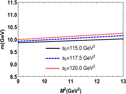
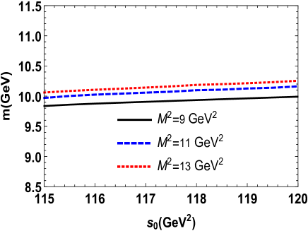
Figure 1: The mass of the tetraquark $T_{bb;\overline{u}\overline{d}}^{-}$ as a function of the Borel parameter (left) and continuum threshold parameter (right).

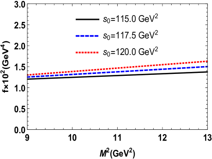
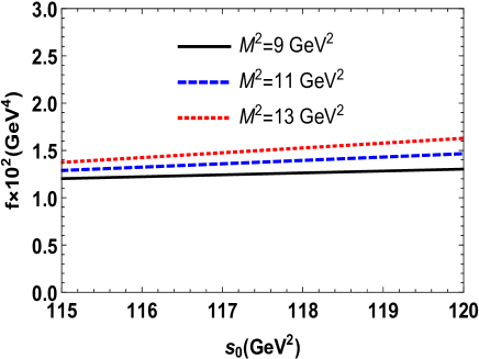
Figure 2: The coupling $f$ vs $M^{2}$ (left) and $s_{0}$ (right).

Our analysis for the mass and coupling of the tetraquark $T_{bb;\overline{d}\overline{u}}^{-}$ predicts

$$m = (10035~{}\pm 260)~{}\mathrm{MeV},$$

$$f = (1.38\pm 0.27)\cdot 10^{-2}\ \mathrm{GeV}^{4}.$$ (18)

Similar studies of $Z_{bc}^{0}$ lead to the following results:

$$m_{Z} = (6660\pm 150~{})\ \mathrm{MeV},$$

$$f_{Z} = (0.51\pm 0.16)\cdot 10^{-2}\ \mathrm{GeV}^{4},$$ (19)

which have been obtained using the working regions

$$M^{2}\in[5.5,\ 6.5]\ \mathrm{GeV}^{2},\ s_{0}\in[53,\ 55]\ \mathrm{GeV}^{2}.$$ (20)

It is worth noting that in the calculations of $m_{Z}$ and $f_{Z}$ the $\mathrm{PC}$ by $55$ to $-21\%$. The contribution of the last three terms to the corresponding correlation function at the point $M^{2}=5.5\ \mathrm{GeV}^{2}$ amounts to $1.9\%$ of the total result, which guarantees the convergence of the sum rules. In Figs. 3 and  4 we depict the mass and coupling of the tetraquark $Z_{bc}^{0}$ as a function of $M^{2}$ and $s_{0}$ to demonstrate their residual dependence on these parameters. It is evident that, as in the case of the $T_{bb;\overline{d}\overline{u}}^{-}$ state, the mass $m_{Z}$ is less sensitive to variations of $M^{2}$ and $s_{0}$ than the coupling $f_{Z}$. But, the relevant theoretical errors stay within the allowed limits inherent to sum rule computations, which may equal up to $\pm 30\%$ of the predictions.

As it has been noted above, the mass of the state $T_{bb;\overline{u}\overline{d}}^{-}$ was evaluated using different approaches in Refs. Navarra:2007yw ; Du:2012wp and Karliner:2017qjm . The investigations in the first two papers were carried out in the framework of the sum rules method, therefore we first compare our result for $m$ with those predictions. Our result for $m$ is smaller than the prediction $m=10.2\pm 0.3\ \mathrm{GeV}$ made in Ref. Navarra:2007yw : there is an overlapping region between these two results, but the central values differ from each other. This discrepancy is presumably connected with the accuracy of the analysis performed there (up to dimension-eight condensates), and with the choice of the working intervals for the parameters $M^{2}$ and $s_{0}$. Thus, in Ref. Navarra:2007yw the explored range for the continuum threshold was $11.3\leq\sqrt{s_{0}}\leq 11.7$ $\mathrm{GeV}$, whereas the Borel parameter varied within the limits $M^{2}\in[7.5,\ 9.6]\ \mathrm{GeV}^{2}$ or $M^{2}\in[7.5,\ 11.2]\ \mathrm{GeV}^{2}$. Because $\sqrt{s_{0}}$ determines the mass of the first excited tetraquark $T_{bb;\overline{u}\overline{d}}^{-}$ the corresponding mass gap amounts to $\Delta m=1.30\pm 0.36\ \mathrm{GeV}$ which is larger than the typical tetraquark value $\Delta m_{T}\sim 0.5-0.7$ $\mathrm{GeV}$. In our case, this mass gap is $\Delta m=0.79\pm 0.17\ \mathrm{GeV}$ and overshoots $\Delta m_{T}$ as well. But one should take into account that the estimate $\Delta m_{T}\sim 0.6$ $\mathrm{GeV}$ was made for tetraquarks lying near or above the corresponding two-meson thresholds, and therefore this fact may be connected with the stable nature of $T_{bb;\overline{u}\overline{d}}^{-}$.

The sum rules analysis of the state $T_{bb;\overline{u}\overline{d}}^{-}$ was performed in Ref. Du:2012wp by employing various interpolating currents $\eta_{i}$. In computations the continuum threshold $s_{0}=115\ \mathrm{GeV}^{2}$ and different regions for the Borel parameter were used with $M^{2}=[6.5,\ 8.6]\ \mathrm{GeV}^{2}$ and $M^{2}=[7.0,\ 9.2]\ \mathrm{GeV}^{2}$ being two extreme choices for $M^{2}$. The mass of the axial-vector tetraquark $T_{bb;\overline{u}\overline{d}}^{-}$ in Ref. Du:2012wp was found to be $m=10.2\pm 0.3\ \mathrm{GeV}$. Here we also underline a difference between the Borel windows in Ref. Du:2012wp and those in the present work as a possible source of this deviation.

The recent model analysis of Ref. Karliner:2017qjm predicted $m=10389\pm 12\ \mathrm{MeV}$ which is considerably larger than the present result. Nevertheless, all calculations confirm that the tetraquark $T_{bb;\overline{u}\overline{d}}^{-}$ is stable against the strong and electromagnetic decays and can only dissociate weakly.

The tetraquarks $Z_{bc}=[bc][\overline{q}\overline{q}]$ ($q=u,d$) were investigated in Ref. Chen:2013aba by employing the QCD sum rule method and various interpolating currents. The masses of the charged scalar tetraquarks $Z_{bc;\overline{u}\overline{u}}^{-}=[bc][\overline{u}\overline{u}]$ and $Z_{bc;\overline{d}\overline{d}}^{+}=[bc][\overline{d}\overline{d}]$ found there were $m=7.14\pm 0.10$ $\mathrm{GeV}$. This prediction is considerably higher than our present result for $m_{Z}$. But one should take into account that the scalar tetraquark $Z_{bc;\bar{u}\bar{d}}^{0}=[bc][\overline{u}\overline{d}]$ has different quark content: it is a neutral particle and contains [like the resonance $X(5568)$] four quarks of different flavors. Therefore, a discrepancy between the predictions for $Z_{bc}$ and $Z_{bc}^{0}$ may be explained not only by the accuracy of the corresponding sum rule analysis and different working regions for the parameters $M^{2}$ and $s_{0}$, but also by the aforementioned reasons.  In Ref.Feng:2013kea the masses of the ground-state tetraquarks $QQ^{\prime}\overline{u}\overline{d}$ in the context of the Bethe-Salpeter method. In the case of the state $Z_{bc}^{0}$ using one of parameters sets the authors found that its mass is $m=6.93$ $\mathrm{GeV}$: this estimate is closer to our prediction.

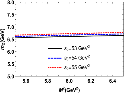
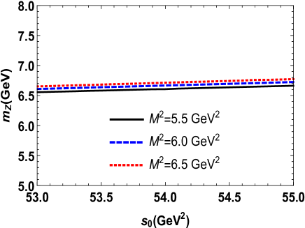
Figure 3: The same as in Fig. 1, but for the mass of the tetraquark $Z_{bc}^{0}$.

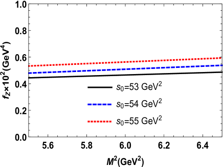
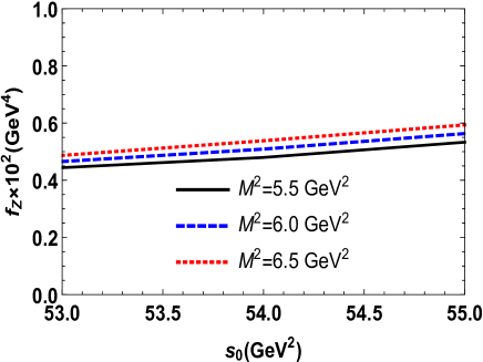
Figure 4: The coupling $f_{Z}$ of the tetraquark $Z_{bc}^{0}$ vs $M^{2}$ (left) and $s_{0}$ (right).

III Semileptonic decay $T_{bb;\overline{u}\overline{d}}^{-}\rightarrow Z_{bc}^{0}l\overline{\nu}_{l}$

The semileptonic decay of the tetraquark $T_{bb;\overline{u}\overline{d}}^{-}$ to the final state $Z_{bc}^{0}l\overline{\nu}_{l}$ runs through the chain of transitions $b\rightarrow W^{-}c$ and $W^{-}\rightarrow l\overline{\nu}$. As is seen from results obtained in the previous section, the difference between the initial and final tetraquarks masses is large enough to make all of the decays $l=e,\ \mu$ and $\tau$ kinematically allowed processes.

At the tree level the transition $b\rightarrow c$ can be described using the effective Hamiltonian

$$\mathcal{H}^{\mathrm{eff}}=\frac{G_{F}}{\sqrt{2}}V_{bc}\overline{c}\gamma_{\mu}(1-\gamma_{5})b\overline{l}\gamma^{\mu}(1-\gamma_{5})\nu_{l},$$ (21)

where $G_{F}$ is the Fermi coupling constant and $V_{bc}$ is the corresponding element of the Cabibbo-Kobayashi-Maskawa (CKM) matrix. After sandwiching the $\mathcal{H}^{\mathrm{eff}}$ between the initial and final tetraquarks and factoring out the lepton fields we get the matrix element of the current

$$J_{\mu}^{\mathrm{tr}}=\overline{c}\gamma_{\mu}(1-\gamma_{5})b$$ (22)

in terms of the form factors $G_{i}(q^{2})$ that parametrize the long-distance dynamics of the weak transition Ball:1991bs

$$\langle Z(p^{\prime})|J_{\mu}^{\mathrm{tr}}|T(p,\epsilon)\rangle=\widetilde{G}_{0}(q^{2})\epsilon_{\mu}+\widetilde{G}_{1}(q^{2})(\epsilon p^{\prime})P_{\mu}$$

$$+\widetilde{G}_{2}(q^{2})(\epsilon p^{\prime})q_{\mu}+i\widetilde{G}_{3}(q^{2})\varepsilon_{\mu\nu\alpha\beta}\epsilon^{\nu}p^{\alpha}p^{\prime}{}^{\beta}.$$ (23)

The scaled functions $\widetilde{G}_{i}(q^{2})$ above are connected with the dimensionless form factors $G_{i}(q^{2})$ by the following equalities

$$\widetilde{G}_{0}(q^{2})=\widetilde{m}G_{0}(q^{2}),\ \widetilde{G}_{j}(q^{2})=\frac{G_{j}(q^{2})}{\widetilde{m}},\ j=1,2,3.$$ (24)

In Eqs. (23) and  (24) $\widetilde{m}=m+m_{Z},\ p$ and $\epsilon$ are the momentum and polarization vector of the tetraquark $T_{bb;\overline{u}\overline{d}}^{-}$, $p^{\prime}$ is the momentum of the state $Z_{bc}^{0}$, $P_{\mu}=p_{\mu}^{\prime}+p_{\mu}$, and $q_{\mu}=p_{\mu}-p_{\mu}^{\prime}$ is the momentum transferred to the leptons. It is clear that $q^{2}$ changes within the limits $m_{l}^{2}\leq q^{2}\leq(m-m_{Z})^{2},$ where $m_{l}$ is the mass of the lepton $l$.

The form factors $G_{i}(q^{2})$ are quantities that should be extracted from the sum rules which, in turn, are obtainable from an analysis of the three-point correlation function

$$\Pi_{\mu\nu}(p,p^{\prime}) = i^{2}\int d^{4}xd^{4}ye^{i(p^{\prime}y-px)}$$ (25)

$$\times\langle 0|\mathcal{T}\{J^{Z}(y)J_{\mu}^{\mathrm{tr}}(0)J_{\nu}^{{}^{\dagger}}(x)\}|0\rangle,$$

where $J_{\nu}(x)$ and $J^{Z}(y)$ are the interpolating currents to the $T_{bb;\overline{u}\overline{d}}^{-}$ and $Z_{bc}^{0}$   states, respectively.

To derive sum rules for the weak form factors we express the correlation function $\Pi_{\mu\nu}(p,p^{\prime})$ in terms of the masses and couplings of the involved particles, and thus determine the physical or phenomenological side of the sum rule $\Pi_{\mu\nu}^{\mathrm{Phys}}(p,p^{\prime})$. We also calculate $\Pi_{\mu\nu}(p,p^{\prime})$ using the interpolating currents and quark propagators, which leads to its expression in terms of the quark, gluon, and mixed vacuum condensates. By matching the obtained results and employing the assumption on the quark-hadron duality, it is possible to extract sum rules and evaluate the physical parameters of interest.

The function $\Pi_{\mu\nu}^{\mathrm{Phys}}(p,p^{\prime})$ can be easily written down in the form

$$\Pi_{\mu\nu}^{\mathrm{Phys}}(p,p^{\prime})=\frac{\langle 0|J^{Z}|Z(p^{\prime})\rangle\langle Z(p^{\prime})|J_{\mu}^{\mathrm{tr}}|T(p,\epsilon)\rangle}{(p^{2}-m^{2})(p^{\prime 2}-m_{Z}^{2})}$$

$$\times\langle T(p,\epsilon)|J_{\nu}^{{}^{\dagger}}|0\rangle+\ldots,$$ (26)

where we only take into account contribution arising from the ground-state particles, and effects of the excited and continuum states are denoted by dots.

The phenomenological side of the sum rules can be further simplified by rewriting the relevant matrix elements in terms of the tetraquarks parameters, and employing for $\langle Z(p^{\prime})|J_{\mu}^{\mathrm{tr}}|T(p,\epsilon)\rangle$ its expression through the weak transition form factors $G_{i}(q^{2})$. The matrix elements of the tetraquarks $T_{bb;\overline{u}\overline{d}}^{-}$ and $Z_{bc}^{0}$ are known and given by Eqs. (6) and (14), respectively. The matrix element $\langle Z(p^{\prime})|J_{\mu}^{\mathrm{tr}}|T(p,\epsilon)\rangle$ is modeled by means of the four transition form factors $G_{i}(q^{2})$ which can be used to calculate all three semileptonic decays.

Substituting the relevant matrix elements into Eq. (26), for $\Pi_{\mu\nu}^{\mathrm{Phys}}(p,p^{\prime},q^{2})$ we finally get

$$\Pi_{\mu\nu}^{\mathrm{Phys}}(p,p^{\prime},q^{2})=\frac{fmf_{Z}m_{Z}}{(p^{2}-m^{2})(p^{\prime 2}-m_{Z}^{2})}$$

$$\times\left\{\widetilde{G}_{0}(q^{2})\left(-g_{\mu\nu}+\frac{p_{\mu}p_{\nu}}{m^{2}}\right)+\left[\widetilde{G}_{1}(q^{2})P_{\mu}\right.\right.$$

$$\left.+\widetilde{G}_{2}(q^{2})q_{\mu}\right]\left(-p_{\nu}^{\prime}+\frac{m^{2}+m_{Z}^{2}-q^{2}}{2m^{2}}p_{\nu}\right)$$

$$\left.-i\widetilde{G}_{3}(q^{2})\varepsilon_{\mu\nu\alpha\beta}p^{\alpha}p^{\prime}{}^{\beta}\right\}+\ldots$$ (27)

The function $\Pi_{\mu\nu}^{\mathrm{OPE}}(p,p^{\prime})$ constitutes the second side of the sum rules and has the following form

$$\Pi_{\mu\nu}^{\mathrm{OPE}}(p,p^{\prime})=\int d^{4}xd^{4}ye^{i(p^{\prime}y-px)}\left\{\mathrm{Tr}\left[\gamma_{5}\widetilde{S}_{d}^{b^{\prime}b}(x-y)\right.\right.$$

$$\left.\times\gamma_{5}S_{u}^{a^{\prime}a}(x-y)\right]\left(\mathrm{Tr}\left[\gamma_{\mu}\widetilde{S}_{b}^{aa^{\prime}}(y-x)\gamma_{5}S_{c}^{bi}(y)\gamma_{\nu}(1-\gamma_{5})\right.\right.$$

$$\left.\times S_{b}^{ib^{\prime}}(-x)\right]+\mathrm{Tr}\left[\gamma_{\mu}\widetilde{S}_{b}^{ia^{\prime}}(-x)(1-\gamma_{5})\gamma_{\nu}\widetilde{S}_{c}^{bi}(y)\gamma_{5}\right.$$

$$\left.\left.\times S_{b}^{ab^{\prime}}(y-x)\right]\right)-\mathrm{Tr}\left[\gamma_{5}\widetilde{S}_{d}^{b^{\prime}a}(x-y)\gamma_{5}S_{u}^{a^{\prime}b}(x-y)\right]$$

$$\times\left(\mathrm{Tr}\left[\gamma_{\mu}\widetilde{S}_{b}^{aa^{\prime}}(y-x)\gamma_{5}S_{c}^{bi}(y)\gamma_{\nu}(1-\gamma_{5})S_{b}^{ib^{\prime}}(-x)\right]\right.$$

$$\left.\left.+\mathrm{Tr}\left[\gamma_{\mu}\widetilde{S}_{b}^{ia^{\prime}}(-x)(1-\gamma_{5})\gamma_{\nu}\widetilde{S}_{c}^{bi}(y)\gamma_{5}S_{b}^{ab^{\prime}}(y-x)\right]\right)\right\}.$$

To extract the sum rules for the form factors $G_{i}(q^{2})$ we equate invariant amplitudes corresponding to the same Lorentz structures in $\Pi_{\mu\nu}^{\mathrm{Phys}}(p,p^{\prime},q^{2})$ and $\Pi_{\mu\nu}^{\mathrm{OPE}}(p,p^{\prime})$, perform a double Borel transformation over the variables $p^{\prime 2}$ and $p^{2}$ to suppress contributions of the higher excited and continuum states, and perform continuum subtraction. For example, to extract the sum rule for $\widetilde{G}_{0}(q^{2})$ we use the structure $g_{\mu\nu}$, whereas for $\widetilde{G}_{3}(q^{2})$ we employ the term $\sim\varepsilon_{\mu\nu\alpha\beta}p^{\alpha}p^{\prime}{}^{\beta}$. It is convenient to present the obtained sum rules in a single formula through the functions $\widetilde{G}_{i}(q^{2})$,

$$\widetilde{G}_{i}(\mathbf{M}^{2},\ \mathbf{s}_{0},~{}q^{2})=\frac{1}{fmf_{Z}m_{Z}}\int_{4m_{b}^{2}}^{s_{0}}ds\int_{(m_{b}+m_{c})^{2}}^{s_{0}^{\prime}}ds^{\prime}$$

$$\times\rho_{i}(s,s^{\prime},q^{2})e^{(m^{2}-s)/M_{1}^{2}}e^{(m_{Z}^{2}-s^{\prime})/M_{2}^{2}},$$ (29)

bearing in mind that they are connected to the dimensionless form factors $G_{i}(q^{2})$ by Eq. (24). Here $\mathbf{M}^{2}=(M_{1}^{2},\ M_{2}^{2})$ are the Borel parameters, and $\mathbf{s}_{0}=(s_{0},\ s_{0}^{\prime})$ are the continuum threshold parameters that separate the main contribution to the sum rules from the continuum effects. The sum rules (29) are written down using the spectral densities $\rho_{i}(s,s^{\prime},q^{2})$ which are proportional to the imaginary parts of the corresponding invariant amplitudes in $\Pi_{\mu\nu}^{\mathrm{OPE}}(p,p^{\prime})$. They contain the perturbative and nonperturbative contributions, and are calculated with dimension-six accuracy.

For numerical computations of the weak form factors $G_{i}(\mathbf{M}^{2},\ \mathbf{s}_{0},~{}q^{2})$ one needs to fix various parameters. Values some of these parameters are collected in Table 1, while the masses and coupling constants of the tetraquarks $T_{bb;\overline{u}\overline{d}}^{-}$ and $Z_{bc}^{0}$ were evaluated in the previous section. In the present computations we impose the same constraints on the auxiliary parameters $\mathbf{M}^{2}$ and $\mathbf{s}_{0}$ as in the mass calculations.

To obtain the width of the decay $T_{bb;\overline{u}\overline{d}}^{-}\rightarrow Z_{bc}^{0}l\overline{\nu}_{l}$ one has to integrate the differential decay rate $d\Gamma/dq^{2}$ (for details, see the Appendix) within allowed kinematical limits $m_{l}^{2}\leq q^{2}\leq(m-m_{Z})^{2}$. It is clear that for light leptons $l=e,\ \mu$ the lower limit of the integral is considerably smaller than $1\ \mathrm{GeV}^{2}$, but the perturbative calculations lead to reliable predictions for momentum transfers $q^{2}>1\ \mathrm{GeV}^{2}$. Therefore, we use the usual prescription and replace the weak form factors in the whole integration region by fit functions $F_{i}(q^{2})$ which for perturbatively allowed values of $q^{2}$ coincide with $G_{i}(q^{2})$.

There are various analytical expressions for the fit functions. In the present paper we utilize

$$F_{i}(q^{2})=f_{0}^{i}\exp\left[c_{1i}\frac{q^{2}}{m_{\mathrm{fit}}^{2}}+c_{2i}\left(\frac{q^{2}}{m_{\mathrm{fit}}^{2}}\right)^{2}\right],$$ (30)

where $f_{0}^{i},~{}c_{1i},\ c_{2i}$ and $m_{\mathrm{fit}}^{2}$ are fitting parameters. The values of these parameters are presented in Table 2. Besides that, for the numerical calculations we need the Fermi coupling constant $G_{F}$ and CKM matrix element $|V_{bc}|$ for which we use

$$G_{F} = 1.16637\cdot 10^{-5}\ \mathrm{GeV}^{-2},\$$

$$|V_{bc}| = (41.2\pm 1.01)\cdot 10^{-3}.$$ (31)

$F_{i}(q^{2})$	$f_{0}^{i}$	$c_{1i}$	$c_{2i}$	$m^{2}_{\mathrm{fit}}\ (\mathrm{GeV}^{2})$
$F_{0}(q^{2})$	$-2.34$	$19.53$	$-36.87$	$100.70$
$F_{1}(q^{2})$	$-1.75$	$18.45$	$-14.29$	$100.70$
$F_{2}(q^{2})$	$8.80$	$20.21$	$-32.09$	$100.70$
$F_{3}(q^{2})$	$17.13$	$20.60$	$-32.49$	$100.70$

Table 2: The parameters of the fit functions $F_{i}(q^{2})$.

As a result, for the decay width of the processes $T_{bb;\overline{u}\overline{d}}^{-}\rightarrow Z_{bc}^{0}l\overline{\nu}_{l},\ (l=e,\ \mu$ and $\tau)$ we find

$$\Gamma\left(T_{bb;\overline{u}\overline{d}}^{-}\rightarrow Z_{bc}^{0}e\overline{\nu}_{e}\right)=\left(2.65\pm 0.78\right)\cdot 10^{-8\ \ }\mathrm{MeV},$$

$$\Gamma\left(T_{bb;\overline{u}\overline{d}}^{-}\rightarrow Z_{bc}^{0}\mu\overline{\nu}_{\mu}\right)=\left(2.64\pm 0.78\right)\cdot 10^{-8\ \ }\mathrm{MeV},$$

$$\Gamma\left(T_{bb;\overline{u}\overline{d}}^{-}\rightarrow Z_{bc}^{0}\tau\overline{\nu}_{\tau}\right)=\left(1.88\pm 0.55\right)\cdot 10^{-8\ }\mathrm{MeV},$$

(32)

which are the main results of the present work.

The partial decay widths from Eq. (32) can be used to estimate the full width and mean lifetime of the tetraquark $T_{bb;\overline{u}\overline{d}}^{-}$

$$\Gamma = (7.17\pm 1.23)\cdot 10^{-8\ \ }\mathrm{MeV},$$

$$\tau = 9.18_{-1.34}^{+1.90}\cdot 10^{-15}\ \mathrm{s.}$$ (33)

These predictions can be employed to explore the double-heavy tetraquarks.

IV Analysis and conclusions

The spectroscopic parameters of the tetraquarks $T_{bb;\overline{u}\overline{d}}^{-}$ and $Z_{bc}^{0}$ as well as the width of the semileptonic decay $T_{bb;\overline{u}\overline{d}}^{-}\rightarrow Z_{bc}^{0}l\overline{\nu}_{l}$ provide very interesting information on the properties of four-quark systems. Thus, the mass of the tetraquark $T_{bb;\overline{u}\overline{d}}^{-}$ obtained in the present work confirms once more that it is stable against strong and electromagnetic decays, and can transform only weakly to a tetraquark $Z_{bc}^{0}$ and a pair of leptons $l\overline{\nu}_{l}$. This conclusion is valid even when taking into account uncertainties inherent to the sum rule computations. Our result for $m$ is smaller than the predictions made in Refs. Navarra:2007yw and Karliner:2017qjm using the QCD sum rule method and phenomenological model estimations, respectively. The semileptonic decays $T_{bb;\overline{u}\overline{d}}^{-}\rightarrow Z_{bc}^{0}l\overline{\nu}_{l}$, where $l=e,\ \mu$ and $\tau$ have allowed us to evaluate the width of $T_{bb;\overline{u}\overline{d}}^{-}$ and its mean lifetime $\tau=9.18_{-1.34}^{+1.90}~{}\mathrm{fs}$ which is considerably shorter than the prediction of Ref. Karliner:2017qjm .

Another interesting result of this work is connected with the parameters of the scalar tetraquark $Z_{bc}^{0}$ composed of the heavy diquark $bc$ and light antidiquark $\overline{u}\overline{d}$. In fact, the mass of this state $m_{Z}=(6660\pm 150~{})\ \mathrm{MeV}$ is considerably below the threshold $\approx 7145\ \mathrm{MeV}$ for strong $S$-wave decays to conventional heavy $B^{-}D^{+}$ and $\overline{B^{0}}D^{0}$ mesons. Because of its quark content. $Z_{bc}^{0}$ cannot decay to a pair of heavy and light mesons as well. These features differ qualitatively from those of the open charm-bottom scalar tetraquarks $Z_{q}=[cq][\overline{b}\overline{q}]$ and $Z_{s}=[cs][\overline{b}\overline{s}]$, which decay strongly to $B_{c}\pi$ and $B_{c}\eta$ mesons Agaev:2016dsg , and, in turn, cannot decay to two heavy mesons. In other words, the four-quark system consisting of a heavy diquark and a light antidiquark is more stable than one consisting of a heavy-light diquark and antidiquark. This is seen from a comparison of the masses of the tetraquark $Z_{bc}^{0}$ and the state $Z_{q}$, for which $m_{Z_{q}}=(6.97\pm 0.19)~{}\mathrm{GeV}$.

Theoretical information on the decay properties of the state $T_{bb;\overline{u}\overline{d}}^{-}$ can be further improved by including its other weak decay channels in analyses. The investigation of the stable open charm-bottom tetraquarks $Z_{bc}^{0}$ with different quantum numbers is also an interesting topic of exotic hadron physics: by clarifying these problems we can deepen our understanding of multiquark systems.

Appendix A The decay rate $d\Gamma/dq^{2}$

This appendix contains the explicit expression for the decay rate $d\Gamma/dq^{2}$ necessary to calculate the width of the semileptonic decay $T_{bb;\overline{u}\overline{d}}^{-}\rightarrow Z_{bc}^{0}l\overline{\nu}_{l}$. Calculations lead to the following result:

$$\frac{d\Gamma}{dq^{2}}=\frac{G_{F}^{2}|V_{cb}|^{2}}{3\cdot 2^{8}\pi^{3}m^{3}}\left(\frac{q^{2}-m_{l}^{2}}{q^{2}}\right)\lambda\left(m^{2},m_{Z}^{2},q^{2}\right)\left[\sum_{i=0}^{i=3}\widetilde{G}_{i}^{2}(q^{2})\mathcal{A}_{i}(q^{2})+\widetilde{G}_{0}(q^{2})\widetilde{G}_{1}(q^{2})\mathcal{A}_{01}(q^{2})\right.$$

$$\left.+\widetilde{G}_{0}(q^{2})\widetilde{G}_{2}(q^{2})\mathcal{A}_{02}(q^{2})+\widetilde{G}_{1}(q^{2})\widetilde{G}_{2}(q^{2})\mathcal{A}_{12}(q^{2})\right.\bigg{]},$$ (A.34)

In Eq. (A.34) the functions $\mathcal{A}_{i}(q^{2})$ and $\mathcal{A}_{ij}(q^{2})$ are given by

$$\mathcal{A}_{0}(q^{2}) = \frac{1}{2m^{2}q^{4}}\left[q^{4}\left(m^{2}-m_{Z}^{2}\right)^{2}-4q^{4}m^{2}m_{l}^{2}-m_{l}^{4}\left(m^{2}-m_{Z}^{2}+q^{2}\right)^{2}+2q^{6}\left(3m^{2}-m_{Z}^{2}\right)+q^{8}\right],$$

$$\mathcal{A}_{1}(q^{2}) = \frac{1}{2m^{2}q^{4}}\left[m^{4}+\left(m_{Z}^{2}-q^{2}\right)^{2}-2m^{2}(m_{Z}^{2}+q^{2})\right]\left\{m_{l}^{4}(m^{2}-m_{Z}^{2})^{2}+q^{4}m_{l}^{4}(q^{2}-2m^{2}-2m_{Z}^{2})\right.$$

$$\left.-q^{4}\left[m^{4}+(m_{Z}^{2}-q^{2})^{2}-2m^{2}(m_{Z}^{2}+q^{2})\right]\right\},$$

$$\mathcal{A}_{2}(q^{2}) = \frac{m_{l}^{2}}{2m^{2}}\left(q^{2}-m_{l}^{2}\right)\left[m^{4}+(m_{Z}^{2}-q^{2})^{2}-2m^{2}(m_{Z}^{2}+q^{2})\right],$$

$$\mathcal{A}_{3}(q^{2}) = \frac{1}{2q^{2}}(m_{l}^{4}-q^{4})\left[m^{4}+(m_{Z}^{2}-q^{2})^{2}-2m^{2}(m_{Z}^{2}+q^{2})\right],$$

$$\mathcal{A}_{01}(q^{2}) = \frac{1}{m^{2}q^{4}}\left[q^{4}(m_{l}^{2}+m_{Z}^{2}-m^{2}-q^{2})+m_{l}^{4}(m^{2}-m_{Z}^{2})\right]\left[m^{4}+(m_{Z}^{2}-q^{2})^{2}-2m^{2}(m_{Z}^{2}+q^{2})\right],$$

$$\mathcal{A}_{02}(q^{2}) = \frac{m_{l}^{2}(m_{l}^{2}-q^{2})}{m^{2}q^{2}}\left[m^{4}+(m_{Z}^{2}-q^{2})^{2}-2m^{2}(m_{Z}^{2}+q^{2})\right],$$

$$\mathcal{A}_{12}(q^{2}) = \frac{m_{l}^{2}(q^{2}-m_{l}^{2})(m^{2}-m_{Z}^{2})}{m^{2}q^{2}}\left[m^{4}+(m_{Z}^{2}-q^{2})^{2}-2m^{2}(m_{Z}^{2}+q^{2})\right],$$ (A.35)

and

$$\lambda\left(m^{2},m_{Z}^{2},q^{2}\right)=\left[m^{4}+m_{Z}^{4}+q^{4}-2\left(m^{2}m_{Z}^{2}+m^{2}q^{2}+m_{Z}^{2}q^{2}\right)\right]^{1/2}.$$

References

• (1) R. L. Jaffe, Phys. Rev. D 15, 267 (1977).
• (2) R. L. Jaffe, Phys. Rev. D 15, 281 (1977).
• (3) J. D. Weinstein and N. Isgur, Phys. Rev. Lett. 48, 659 (1982).
• (4) J. P. Ader, J. M. Richard and P. Taxil, Phys. Rev. D 25, 2370 (1982).
• (5) H. X. Chen, W. Chen, X. Liu and S. L. Zhu, Phys. Rept. 639, 1 (2016).
• (6) A. Esposito, A. Pilloni and A. D. Polosa, Phys. Rept. 668, 1 (2017).
• (7) A. Ali, J. S. Lange and S. Stone, Prog. Part. Nucl. Phys. 97, 123 (2017).
• (8) S. L. Olsen, T. Skwarnicki and D. Zieminska, Rev. Mod. Phys. 90, 015003 (2018).
• (9) H. J. Lipkin, Phys. Lett. B 172, 242 (1986).
• (10) S. Zouzou, B. Silvestre-Brac, C. Gignoux and J. M. Richard, Z. Phys. C 30, 457 (1986).
• (11) J. Carlson, L. Heller and J. A. Tjon, Phys. Rev. D 37, 744 (1988).
• (12) A. V. Manohar and M. B. Wise, Nucl. Phys. B 399, 17 (1993).
• (13) S. Pepin, F. Stancu, M. Genovese and J. M. Richard, Phys. Lett. B 393, 119 (1997).
• (14) D. Janc and M. Rosina, Few Body Syst. 35, 175 (2004).
• (15) Y. Cui, X. L. Chen, W. Z. Deng and S. L. Zhu, HEPNP 31, 7 (2007).
• (16) J. Vijande, A. Valcarce and K. Tsushima, Phys. Rev. D 74, 054018 (2006).
• (17) D. Ebert, R. N. Faustov, V. O. Galkin and W. Lucha, Phys. Rev. D 76, 114015 (2007).
• (18) F. S. Navarra, M. Nielsen and S. H. Lee, Phys. Lett. B 649, 166 (2007).
• (19) M. L. Du, W. Chen, X. L. Chen and S. L. Zhu, Phys. Rev. D 87, 014003 (2013).
• (20) J. Schaffner-Bielich and A. P. Vischer, Phys. Rev. D 57, 4142 (1998).
• (21) A. Del Fabbro, D. Janc, M. Rosina and D. Treleani, Phys. Rev. D 71, 014008 (2005).
• (22) S. H. Lee, S. Yasui, W. Liu and C. M. Ko, Eur. Phys. J. C 54, 259 (2008).
• (23) T. Hyodo, Y. R. Liu, M. Oka, K. Sudoh and S. Yasui, Phys. Lett. B 721, 56 (2013).
• (24) A. Esposito, M. Papinutto, A. Pilloni, A. D. Polosa and N. Tantalo, Phys. Rev. D 88, 054029 (2013).
• (25) R. Aaij et al. [LHCb Collaboration], Phys. Rev. Lett. 119, 112001 (2017).
• (26) M. Karliner and J. L. Rosner, Phys. Rev. Lett. 119, 202001 (2017).
• (27) S. Q. Luo, K. Chen, X. Liu, Y. R. Liu and S. L. Zhu, Eur. Phys. J. C 77, 709 (2017).
• (28) E. J. Eichten and C. Quigg, Phys. Rev. Lett. 119, 202002 (2017).
• (29) Z. G. Wang and Z. H. Yan, Eur. Phys. J. C 78, 19 (2018).
• (30) A. Ali, A. Y. Parkhomenko, Q. Qin and W. Wang, Phys. Lett. B 782, 412 (2018).
• (31) A. Ali, Q. Qin and W. Wang, Phys. Lett. B 785, 605 (2018).
• (32) E. Eichten and Z. Liu, arXiv:1709.09605.
• (33) C. Hughes, E. Eichten and C. T. H. Davies, Phys. Rev. D 97, 054505 (2018).
• (34) A. Esposito and A. D. Polosa, Eur. Phys. J. C 78, 782 (2018).
• (35) S. S. Agaev, K. Azizi, B. Barsbay and H. Sundu, Nucl. Phys. B 939, 130 (2019).
• (36) H. Sundu, B. Barsbay, S. S. Agaev and K. Azizi, Eur. Phys. J. A 54, 124 (2018).
• (37) Y. Xing and R. Zhu, Phys. Rev. D 98, 053005 (2018).
• (38) B. Silvestre-Brac and C. Semay, Z. Phys. C 59, 457 (1993).
• (39) Z. F. Sun, X. Liu, M. Nielsen and S. L. Zhu, Phys. Rev. D 85, 094008 (2012).
• (40) R. M. Albuquerque, X. Liu and M. Nielsen, Phys. Lett. B 718, 492 (2012).
• (41) W. Chen, T. G. Steele and S. L. Zhu, Phys. Rev. D 89, 054037 (2014).
• (42) J. R. Zhang and M. Q. Huang, Phys. Rev. D 80, 056004 (2009).
• (43) J. R. Zhang and M. Q. Huang, Commun. Theor. Phys. 54, 1075 (2010).
• (44) S. S. Agaev, K. Azizi and H. Sundu, Phys. Rev. D 95, 034008 (2017).
• (45) S. S. Agaev, K. Azizi and H. Sundu, Eur. Phys. J. C 77, 321 (2017).
• (46) V. M. Abazov et al. [D0 Collaboration], Phys. Rev. Lett. 117, 022003 (2016).
• (47) G.-Q. Feng, X.-H. Guo and B.-S. Zou, arXiv:1309.7813 [hep-ph].
• (48) P. Ball, V. M. Braun and H. G. Dosch, Phys. Rev. D 44, 3567 (1991).