Exemplar-based synthesis of geology using kernel discrepancies and generative neural networks

Abstract

We propose a framework for synthesis of geological images based on an exemplar image (a.k.a. training image). We synthesize new realizations such that the discrepancy in the patch distribution between the realizations and the exemplar image is minimized. Such discrepancy is quantified using a kernel method for two-sample test called maximum mean discrepancy. To enable fast synthesis, we train a generative neural network in an offline phase to sample realizations efficiently during deployment, while also providing a parametrization of the synthesis process. We assess the framework on a classical binary image representing channelized subsurface reservoirs, finding that the method reproduces the visual patterns and spatial statistics (image histogram and two-point probability functions) of the exemplar image.

1 Introduction

A challenge in subsurface flow simulations is to obtain a complete and accurate image of subsurface properties, such as permeability and porosity, that are crucial for accurate flow predictions. Since it is virtually impossible to obtain direct measurements at every point of the domain under study, engineers can only rely on indirect estimations of the subsurface properties, e.g. from seismic images and sparse measurements obtained from wells. Traditionally, the properties are modeled based on their two-point statistics; however, this tends to produce images of the subsurface that are far from realistic. In many scenarios, such as in channelized systems where the properties follow an almost binary distribution and contain strong spatial correlations, two-point statistics are not enough to describe the distribution of the properties.

This shortcoming led to the development of alternative algorithmic approaches to synthesize subsuface images that can capture multipoint statistics. These methods start from an exemplar image (also called training image in the geology literature) that is deemed representative of the subsurface under study, meaning that the spatial statistics in this image is believed to be similar to that of the subsurface. From there, a new image is synthesized by querying the exemplar image or deriving statistics from it, and employing some form of randomness during the synthesis process to generate diverse outcomes. These methods, although less theoretically founded, tend to produce subsurface images that are more realistic than the traditional methods based on two-point statistics. In [45], empirical conditional probabilities are derived from the exemplar and used to synthesize the new image each pixel at a time. In [27], a pixel is synthesized by simply querying the exemplar and selecting pixels whose neighboring pixels match that of the current synthesized domain. In [46], the synthesis is based on carefully copying and pasting patches extracted from the exemplar. As seen from the mentioned works, these approaches share many similarities with texture synthesis techniques in image processing [7, 6, 26].

A further challenge in subsurface flow simulations is the need to account for inherent uncertainties of the simulations. For uncertainty quantification and history matching, not only is it necessary to explore multiple plausible solutions by performing simulations for a large number of realizations, but also it is desirable that such exploration be smooth in the sense that small changes in input parameters result in small changes in the output. By design, this is not the case in most current synthesis algorithms. For this reason, current approaches take a two-stage process: First, a dataset of realistic realizations is synthesized using one of the many synthesis algorithms available; thereafter, parametrization [39, 24, 15, 50] is performed using the dataset in a way that retains the realism of the realizations while achieving a well-behaved function with respect to new input parameters. It is then worth asking whether it is possible to achieve parametric synthesis directly from the exemplar.

Recent examples of parametric synthesis of geology from a single exemplar include [28, 19] where the authors train generative adversarial networks [10] to parametrize the geology using neural networks, obtaining very impressive results. Generative adversarial networks leverage the representational power of neural networks in two fronts: on one hand, the modeling power of neural networks is leveraged for the realistic parametrization of images; on the other hand, the discriminative power of neural networks is leveraged to learn the statistics of the images. Since training these neural networks still require a dataset of realizations, the approach in [28, 19] is to simply train the neural networks on patches of the exemplar image; once trained, because the neural networks used are convolutional, one can artificially increase the dimension of the input parameter vector to synthesize larger images. However, it remains unclear if this approach generalizes to arbitrary sizes.

Figure 1: Overview of methodology.

In this work, we propose a synthesis method to explicitly reproduce the patch distribution of the exemplar image. Given an exemplar image, we assume that the spatial statistics can be sufficiently described by the distribution of the patches extracted from the exemplar. Note that this assumption is implicit in most exemplar-based synthesis algorithms. Then, new realizations of arbitrary size are synthesized such that their patch distributions match that of the exemplar. The discrepancy in distributions is measured using a kernel method for two-sample test called maximum mean discrepancy (MMD) [13], then new realizations are formulated as solutions to the minimization of this discrepancy. To obtain a parametrization of the synthesis process, as well as improved synthesis speed during the online phase (e.g. for uncertainty quantification or history matching), we assume a Markov random field model where the energy function is (proportional to) the discrepancy, and train a generative neural network in the offline phase to efficiently generate new realizations online. The resulting generator is superficially similar to previous works [28, 19], except that we directly synthesize the desired domain size, the statistics of the synthesized image are explicitly compared to the exemplar, and the comparison is done using a kernel method. An overview of the framework is shown in Figure 1.

In this study, we limit ourselves to the synthesis of unconditional realizations and leave the conditioning case for future work (examples of conditioning to hard data can be found in [4, 29, 2]). We assess our method using the classical binary channelized image by Strebelle [45] of size $250\times 250$, and we synthesize images of size $256\times 256$ and $512\times 512$. We also study the influence of different kernels in the quality of the synthesis and discuss alternatives for improvement. Although not considered here, we note that the framework is dimension-agnostic and can be directly applied to 3D images.

The rest of this work is organized as follows: In Section 2, we describe the maximum mean discrepancy [13], and an approach to train a generative neural network [49]. Our main idea is presented in Section 3: new realizations are formulated as solutions to an optimization problem (minimize the discrepancy in patch distributions); thereafter, a generative neural network can be trained for fast parametric synthesis. In Section 4, we present results for the synthesis of binary channelized subsurface images based on the classical Strebelle exemplar image. In Section 5, we discuss how our framework relates to other works and potential ideas to improve this work. Finally, we state our conclusions and future directions in Section 6.

2 Background

2.1 Maximum mean discrepancy

Our main tool is a kernel method for two-sample test called maximum mean discrepancy [12, 13]. Given two samples $X=\{x_{1},\cdots,x_{m}\}$ and $Y=\{y_{1},\cdots,y_{n}\}$, the goal is to determine whether both samples come from the same distribution. The maximum mean discrepancy (MMD) addresses this problem by comparing the sample mean in a feature space,

$$\operatorname{MMD}^{2}[X,Y] =\left\lVert\frac{1}{m}\sum^{m}_{i=1}\phi(x_{i})-\frac{1}{n}\sum^{n}_{j=1}\phi(y_{j})\right\rVert^{2}_{\mathcal{H}}$$

$$=\frac{1}{m^{2}}\sum^{m}_{i=1}\sum^{m}_{i^{\prime}=1}k(x_{i},x_{i^{\prime}})+\frac{1}{n^{2}}\sum^{n}_{j=1}\sum^{m}_{j^{\prime}=1}k(y_{j},y_{j^{\prime}})-\frac{2}{mn}\sum^{m}_{i=1}\sum^{n}_{j=1}k(x_{i},y_{j})$$ (1)

where $\phi\colon\mathcal{X}\to\mathcal{H}$ is a mapping to the feature space $\mathcal{H}$, and $k(x,y)\coloneqq\langle\phi(x),\phi(y)\rangle_{\mathcal{H}}$. The useful aspect in this formulation is that we do not need to compute $\phi(\cdot)$ – which can be infinite dimensional – as long as we can compute the function $k(\cdot,\cdot)$, called the kernel. The kernel operator can be thought of as a similarity measure, and it must satisfy certain properties in which case it is guaranteed to be associated to some feature mapping/space. For an in-depth treatment, see [13].

Examples

Let $x,y\in\mathbb{R}^{2}$. For the linear kernel $k(x,y)=x^{T}y$, an associated feature map is $\phi(x)=x$, then the MMD is simply the difference in the sample mean. For the polynomial kernel of degree two $k(x,y)=(x^{T}y+1)^{2}$, an associated feature map is $\phi(x)=(x_{(2)}^{2},x_{(1)}^{2},\sqrt{2}x_{(2)}x_{(1)},\sqrt{2}x_{(2)},\sqrt{2}x_{(1)},1)$ where $x=(x_{(1)},x_{(2)})$, then the MMD captures differences in both mean and covariance. Finally, the Gaussian radial basis function $k(x,y)=\exp{\{-\gamma||x-y||^{2}\}}$ is associated with a mapping to infinitely many components (obtained by Taylor expansion) and the corresponding MMD captures all the moments of the distribution.

2.2 Generative neural network

We now describe a method to train a generative neural network as proposed in [49]. Let $g_{\theta}\colon\mathcal{Z}\to\mathcal{X}$ be a neural network parametrized by weights $\theta$ to be determined. The input to the neural network are realizations of a random latent vector $\mathbf{Z}\sim p_{Z}$ that provides the source of stochasticity so that $g_{\theta}(\mathbf{Z})$ is a stochastic simulator. The distribution $p_{Z}$ is a design choice and is usually an easy-to-sample distribution (e.g. standard normal distribution) so that the cost of sampling $g_{\theta}(\mathbf{Z})$ is mostly given by the evaluation cost of $g_{\theta}$. Given a target probability density function $p$, and a fixed $p_{Z}$, the goal is to determine $\theta$ such that $g_{\theta}(\mathbf{Z})\sim p$. Let us denote the density of $g_{\theta}(\mathbf{Z})$ under $\theta$ by $q_{\theta}$. The Kullback-Leibler (KL) divergence from $p$ to $q_{\theta}$ is

$$\operatorname{D_{KL}}(q_{\theta}\parallel p) =\mathop{\mathbb{E}}_{\mathbf{X}\sim q_{\theta}}\log\frac{q_{\theta}(\mathbf{X})}{p(\mathbf{X})}$$ (2)

$$=\mathop{\mathbb{E}}_{\mathbf{X}\sim q_{\theta}}-\log p(\mathbf{X})+\mathop{\mathbb{E}}_{\mathbf{X}\sim q_{\theta}}\log q_{\theta}(\mathbf{X})$$ (3)

We therefore wish to find $\theta$ that minimizes this divergence. The first term of the sum can be approximated as

$$\mathop{\mathbb{E}}_{\mathbf{X}\sim q_{\theta}}-\log p(\mathbf{X})\approx\frac{1}{N}\sum_{i=1}^{N}{-\log p(X_{i})}$$ (4)

where $X_{i}=g_{\theta}(Z_{i})$, by drawing $N$ realizations of $\mathbf{Z}\sim p_{Z}$. The second term of the sum, called the (negative) entropy, is problematic since we do not have the analytic form of the density $q_{\theta}$ ($g_{\theta}$ normally contains multiple non-linearities). We circumvent this issue by using a sample entropy estimator [18, 11] over a set of generated realizations $\{X_{1},\cdots,X_{N}\}$,

$$\mathop{\mathbb{E}}_{\mathbf{X}\sim q_{\theta}}\log q_{\theta}(\mathbf{X})\approx-\hat{H}(\{X_{i},\cdots,X_{N}\})\coloneqq-\frac{1}{N}\sum^{N}_{i=1}c\log\rho(X_{i})+\mathrm{const.}$$ (5)

where $c$ is the number of components of $\mathbf{X}$, and $\rho(X_{i})$ is the distance from $X_{i}$ to its $k^{\mathrm{th}}$-nearest neighbor (with $k\approx\sqrt{N}$ as a good rule of thumb [11]). Essentially, $\hat{H}$ quantifies how spread the realizations are. Putting all together, Equation 2 can be approximated as

$$\operatorname{D_{KL}}(q_{\theta}\parallel p)\approx\frac{1}{N}\sum_{i=1}^{N}{-\log p(X_{i})}-\frac{1}{N}\sum^{N}_{i=1}{c\log\rho(X_{i})}+\mathrm{const.}$$ (6)

Minimizing this expression can be done using gradient-based optimization, where the gradients with respect to $\theta$ can be obtained using automatic differentiation algorithms. Intuitively, the first term ensures that the generated samples are in the regions of high probability of $p$, whereas the second term ensures that the samples are diverse.

3 Methodology

We denote by $X$ an image realization and $\tilde{X}=\{x_{1},\cdots,x_{m}\}$ the corresponding set of patches extracted from $X$. Given an exemplar image $X_{0}$, we assume that the spatial statistics can be sufficiently described by the distribution estimated from the patches $\tilde{X}_{0}=\{x^{0}_{1},\cdots,x^{0}_{n}\}$ extracted from $X_{0}$. We therefore aim to synthesize a new realization $X$ such that the patch distribution estimated from $\tilde{X}=\{x_{1},\cdots,x_{m}\}$ match the patch distribution of the exemplar. For example, matching the distribution of “$1\times 1$ patches” reduces to matching the pixel histogram of the exemplar image. For patches of size $l_{1}\times l_{2}$, the distribution to be matched is given by the multidimensional joint histogram of $l_{1}l_{2}$ variables. The discrepancy in distributions is measured using the maximum mean discrepancy (MMD, Section 2.1), then new realizations are formulated as solutions of an optimization problem,

$$\operatorname*{arg\,min}_{X}{\operatorname{MMD^{2}}[\tilde{X},\tilde{X}_{0}]}$$ (7)

with $\operatorname{MMD^{2}}$ defined in Section 2.1. Note that a patch $x_{i}$ of an image $X$ is the result of a projection operator, therefore the minimization can be done using gradient-based methods. Multiple realizations can be obtained by using a local optimizer and different initial guesses for $X$.

Optimization-based synthesis, however, can be expensive if a large number of realizations is required in the online phase (e.g. for uncertainty quantification or history matching); moreover, it does not provide a smooth parametric way to explore the solution space. We therefore train a generator in an offline phase to synthesize realizations efficiently during deployment. We train the generator following the approach described in Section 2.2, which requires us to define a target density $p$. For this, we shall assume a Markov random field model $p(X)\propto\exp\{-\frac{1}{\lambda}\mathcal{L}(X)\}$ where $\mathcal{L}(X)\coloneqq\operatorname{MMD^{2}}[\tilde{X},\tilde{X}_{0}]$ and $\lambda$ is an unknown “temperature” constant (see [51] or Section 4.1 of [25] for a justification of this choice). This conveniently sets the KL divergence in Equation 2 to

$$\operatorname{D_{KL}}(q_{\theta}\parallel p)\propto\frac{1}{N}\sum_{i=1}^{N}{\mathcal{L}(X_{i})}-\frac{\lambda}{N}\sum^{N}_{i=1}{c\log\rho(X_{i})}$$ (8)

where we multiplied everything by $\lambda$ and omitted the irrelevant constants. The first term ensures that the samples minimize the MMD, while the second term ensures that the samples are diverse. Since we do not know the constant $\lambda$, in this work we treat it as a hyperparameter to be tuned in the offline training. In practice, $\lambda$ acts as the trade-off between sample quality and diversity. We summarize the steps to train the generator in Algorithm 1.

Algorithm 1 Generator training $g_{\theta}$

1: Exemplar image $X_{0}$, kernel $k(\cdot,\cdot)$ of MMD, “temperature” $\lambda$, source distribution $p_{Z}$, batch size $N$.

2:while $\theta$ has not converged do

3:    Sample $\{Z_{1},\cdots,Z_{N}\}\sim p_{Z}$

4:    Obtain $\{X_{1},\cdots,X_{N}\},\;X_{i}=g_{\theta}(Z_{i})$

5:    $\mathbb{E}\mathcal{L}\leftarrow\frac{1}{N}\sum^{N}_{i=1}\operatorname{MMD^{2}}[\tilde{X}_{i},\tilde{X}_{0}]$ $\triangleright$ Section 2.1

6:    $\lambda\hat{H}\leftarrow\frac{\lambda}{N}\sum^{N}_{i=1}c{\log\rho(X_{i})}$

7:    $\theta\leftarrow\operatorname{Update}(\theta;\nabla_{\theta}{(\mathbb{E}\mathcal{L}-\lambda\hat{H})})$

8:end while

3.1 Kernel choice

As in other kernel methods, the kernel choice is critical in the performance of the MMD; specifically, it defines its discriminative power. For characteristic kernels [43, 44], the MMD can distinguish two distributions in the infinite setting [13]. These include the Gaussian radial basis function, the Laplace kernel, and the rational quadratic kernel. In this work, we use the rational quadratic kernel $k_{\mathrm{rq}}(x,y)=(1+\frac{||x-y||^{2}}{2\alpha l^{2}})^{-\alpha}$ due to its better gradient behavior, where $\alpha$ and $l$ are hyperparameters to be tuned during the offline phase (see Section 4.2 of [36] for properties of this and other kernels).

Measuring similarities using kernels, however, can be challenging when the data is very high dimensional [35]. Moreover, distance-based kernels (as functions of $||x-y||$) are not well-suited when applied on the raw pixel representation of images, since differences in pixel values are of little meaning in conveying similarity (e.g. small shifts in pixels would imply large differences while remaining virtually the same). On the other hand, it is often the case that the intrinsic dimensionality of the data is low, albeit embedded in a high dimensional space. For example, geological structures of interest such as channels can be accurately described regardless of the grid resolution, once it is above certain threshold. This suggests us to first project the data to a low dimensional space, e.g. using principal component analysis or even random projections [1], before applying the distance-based kernel. In this work, we use the encoder of an autoencoder trained on patches of the exemplar. The autoencoder [14] is a generalization of principal component analysis using non-linear basis functions (represented by neural networks). The idea here is to measure distances between patches using their code representations instead of their raw pixel representations. The resulting kernel is $k(\cdot,\cdot)=k_{\mathrm{rq}}(h(\cdot),h(\cdot))$ where $h(\cdot)$ denotes the encoder (note that $k_{\mathrm{rq}}(h(\cdot),h(\cdot))$ is a kernel).

4 Numerical experiments

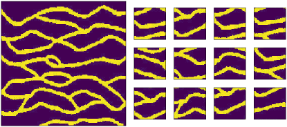
Figure 2: Exemplar image (by Strebelle [45]) of size $250\times 250$ depicting subsurface channels (left), and a few patches of size $64\times 64$ extracted from the image (right).

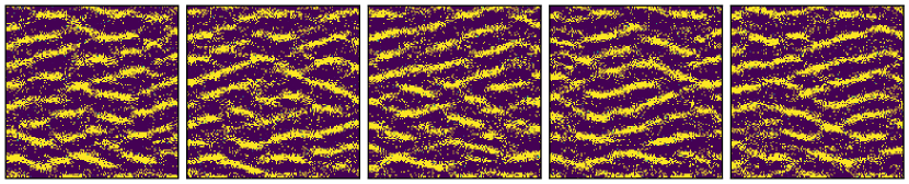
(a) $k_{\mathrm{rq,randproj}}$

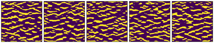
(b) $k_{\mathrm{rq,pca}}$

Figure 3: Optimization-based synthesis using different kernels.

We consider the synthesis of geological realizations containing subsurface channels using the classical exemplar image of Strebelle [45] shown in Figure 2. Note that our target distribution is discrete (the image is binary); nevertheless, we found good results using a continuous framework. For convenience, we pre-process the image and work in the $[-1,1]$ range, so that $-1$ represents the background material (blue) and $1$ represents the channel material (yellow). The size of the exemplar image is $250\times 250$, and we use patches of size $64\times 64$. Naturally, the patch size has to be large enough to capture the relevant patterns of interest in the exemplar image; however, it should not be too large since this determines the amount and variability of patches given that our exemplar is of finite size in practice. We synthesize images of size $256\times 256$ and $512\times 512$.

For the MMD, we use a kernel of the form $k(\cdot,\cdot)=k_{\mathrm{rq}}(h(\cdot),h(\cdot))$ where $h$ is a mapping to a lower dimensional space, and $k_{\mathrm{rq}}$ is the rational quadratic kernel $k_{\mathrm{rq}}(x,y)=1+\frac{||x-y||^{2}}{2\alpha l^{2}})^{-\alpha}$. We use $\alpha=0.5$, and for $l$ (length scale parameter) we use a median heuristic [13]: we use the median distance between the patches in the combined sample – note that this means that our kernel adapts during the training iterations. As for $h$, we experiment with three choices: a random projection matrix [1], principal component analysis (PCA) trained on patches of the exemplar, and the encoder of an autoencoder trained on patches of the exemplar.

Note that the MMD in Section 2.1 has a quadratic cost with respect to the sample size (although linear estimates exist [13]) making it expensive to evaluate in the whole set of patches. Since we compute the MMD iteratively, we instead evaluate on a random subset of patches drawn during the iterations. We draw a subset of $128$ patches. As a consequence, we found that this procedure tends to undersample patches at the boundary of the domain, so we perform reflection padding on the synthesis domain equal to half a patch width before sampling patches – this may introduce some biases at the synthesis boundaries.

Our implementation is done using Pytorch [32], a python package for automatic differentiation.

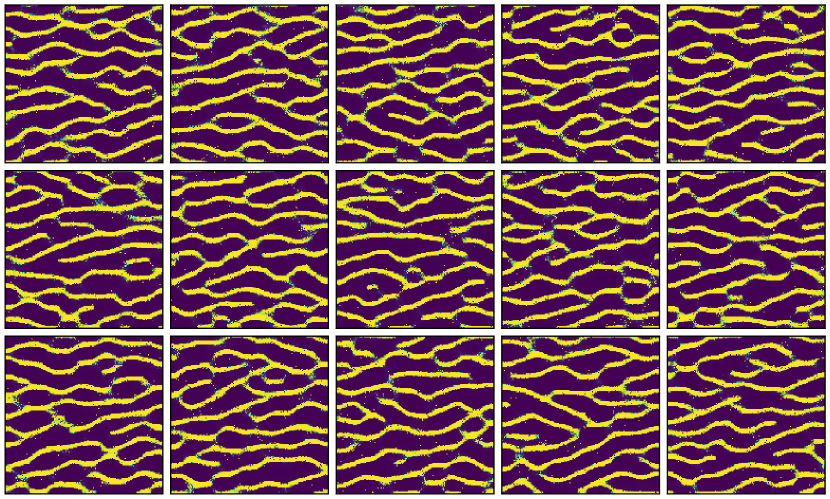
(a) Random realizations ($256\times 256$, optimization-based synthesis).

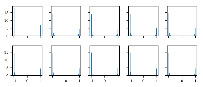
(b) Image histogram of 9 random realizations. The first histogram (top left) corresponds to the exemplar image.

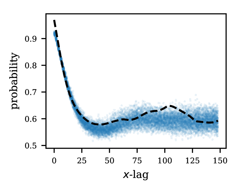
(c) Two-point probability in the $x$ direction of 100 realizations.

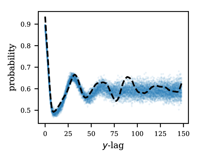
(d) Two-point probability in the $y$ direction of 100 realizations.

Figure 4: Results for optimization-based synthesis of realizations of size $256\times 256$ with $k_{\textrm{rq,encoder}}$ kernel.

4.1 Optimization-based synthesis

We start by synthesizing realizations using an optimization approach (Equation 7). Since the pixel values are bounded in $[-1,1]$, rather than using a constrained optimization method, here we simply reparametrize the pixels by $X=\tanh(X^{\prime})$ and solve for $X^{\prime}$ instead. We use the Adam optimizer [16, 37] (a variant of stochastic gradient descent). We test different kernels for the MMD: For $k_{\mathrm{rq}}$ + random projection ($k_{\textrm{rq,randproj}}$), we use a low-rank random matrix to project each $64\times 64$ patch to a vector of $512$ components. For $k_{\mathrm{rq}}$ + principal component analysis (PCA) ($k_{\textrm{rq,pca}}$), we project each patch to $64$ eigencomponents (retaining over 75% of the variance). Synthesis results for size $256\times 256$ are shown in Figures 3(a) and 3(b). We can see that both random projection and PCA kernels already capture key spatial statistics of the exemplar such as the horizontal correlations defining the channels and the correct pixel values; however, the visual quality of the realizations are still rather poor.

Next, we use the encoder of an autoencoder trained on the patches of the exemplar image ($k_{\textrm{rq,encoder}}$). The autoencoder is trained to encode each patch into a small code vector of size $8$, a number found via experimentation. We experimentally found that smaller codes tend to produce better results (as long as the autoencoder can be trained successfully), presumably by making the distance-based kernel more accurate. Details of the autoencoder implementation are described in Section A.1.

Synthesis results for size $256\times 256$ using the $k_{\mathrm{rq}}$ + encoder kernel are summarized in Figure 4. Compared to the previous kernels, we see that the visual quality of the realizations are significantly improved, highlighting the impact of the kernel choice. The synthesized images, however, still contain some spurious values such as isolated pixels that the optimization did not manage to remove within the iterations. If required, these could be removed using one of many available image post-processing methods [41]. We show in Figure 4(b) the normalized histogram of pixel values of nine random realizations without thresholding, finding good correspondence with the exemplar histogram. We show the two-point probability functions (PF) [47] in the horizontal and vertical directions in Figures 4(c) and 4(d), respectively. The dashed black lines indicate the PFs of the exemplar image, and the dotted blue lines are PFs for $100$ random realizations. We do perform thresholding in this evaluation to compute the PFs. To compute the PFs on the realizations, we randomly crop a region of size $250\times 250$ from each realization in order to match the exemplar size, and compute the PF in this region. Note that before cropping, we first perform a reflection padding as used in the optimization to reduce potential biases at the boundaries. Overall, we find good agreement between the synthesized images and the exemplar. We show additional results for synthesis of size $512\times 512$ in Appendix B.

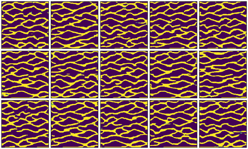
(a) Random realizations ($256\times 256$, generated by neural network).

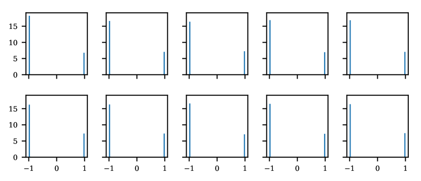
(b) Image histogram of 9 random realizations. The first histogram (top left) corresponds to the exemplar image.

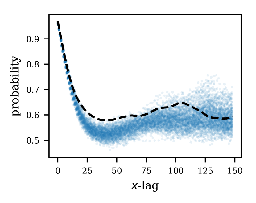
(c) Two-point probability in the $x$ direction of 100 realizations.

(d) Two-point probability in the $y$ direction of 100 realizations.

Figure 5: Results for neural synthesis of realizations of size $256\times 256$ with $k_{\textrm{rq,encoder}}$ kernel.

4.2 Neural synthesis

We next train a generative neural network to synthesize realizations efficiently. Here we only consider the kernel with the encoder of the autoencoder ($k_{\mathrm{rq,encoder}}$). The generator is a convolutional neural network designed following the template provided in [34], which works well for most computer vision tasks. Details of the architecture are given in Section A.2. To synthesize $256\times 256$ images, the generator $g_{\theta}\colon\mathbb{R}^{256}\to\mathbb{R}^{256\times 256}$ maps from realizations of a latent vector of size $256$ sampled from the standard normal distribution, to image realizations of size $256\times 256$. The size of the latent vector was chosen using a simple heuristic: proportional to the number of non-overlapping patches in the synthesis domain times the encoding size. We train $g_{\theta}$ to minimize the KL divergence in Equation 8, where we use a batch size of $N=4$ and temperature hyperparameter $\lambda={10^{-8}}$. We found that a good initial guess for $\lambda$ is a number such that the value of the first and second terms in the KL (expected loss and entropy, respectively) stay within the same order of magnitude in the latter iterations of the training, so that the KL is eventually allowed to go to zero. In fact, here we tuned $\lambda$ from $\{10^{-7},10^{-8},10^{-9}\}$, although finer tuning is encouraged.

Results of the neural synthesis are summarized in Figure 5. Notably, we find that the results using neural synthesis are visually better, e.g. we do not find isolated pixels as in the optimization approach. This can be explained by the locality prior imposed by the convolutional architecture [40, 48]: since the image is parametrized by a neural network, updates in the weights of the neural network affects a whole neighborhood of the output image, in contrast to optimization in the pixel space where pixels are updated individually; moreover, this influence is hierarchical due to the convolutional architecture, since layers closer to the output have a more local influence while layers closer to the input affect the output more globally. Regarding the normalized image histogram (again without thresholding) in Figure 5(b), we find that it more closely matches the true binary shape of the exemplar histogram. Finally, we show the two-point probability functions for the neural synthesis (computed as in the previous section) in Figures 5(c) and 5(d). We find a slight bias in the trend of the curves, which may suggest that further tuning of the neural network is necessary. Nonetheless, the results remain close in relative value.

We additionally train a generator $g_{\theta}\colon\mathbb{R}^{512}\to\mathbb{R}^{512\times 512}$ to synthesize realizations of size $512\times 512$. For this case, we use a latent vector of size $512$ (also with standard normal distribution) and $\lambda=10^{-9}$. The results are summarized in Appendix B.

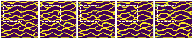
Figure 6: Linear interpolation of one coordinate of the latent vector.

Smooth transitions

Since $g_{\theta}$ is continuous by construction, small changes in the input results in small changes in the output. We verify this in Figure 6 where we show the outputs of the generator of size $256\times 256$. Starting from an initial random realization of the latent vector $\mathbf{Z}$, we linearly vary one of its coordinates while fixing the remaining coordinates. Note that unlike methods such as principal component analysis where the latent vector represents the coefficients of the eigenvectors, the latent vector of generative neural networks lack interpretability. Learning interpretable latent vectors is an ongoing area of research, see e.g. [3].

5 Related work

Neural kernels

The seminal work in [9] showed that it is possible to synthesize textures from an exemplar by matching statistics of feature responses of a pre-trained neural network evaluated on the exemplar. Briefly, the exemplar is fed into the VGG-net [42] – a very large neural network trained on natural images for classification – and a matrix is formed containing the correlations of feature responses at layers of the neural network. Then, new realizations are synthesized such that their corresponding matrices are close to that of the exemplar. It was later shown in [21] that this is equivalent to computing the maximum mean discrepancy on the feature responses using the polynomial kernel $k(x,y)=(x^{T}y)^{2}$. Finally, by noting that each feature response corresponds to a patch of the domain (defined by its receptive field), we conclude that this is an instance of our framework where the kernel is composed of a polynomial kernel and the VGG-net as “encoder”. Note that in this case, the encoder is trained on a different task (classification) using large sets of other images, making the approach an example of transfer learning [33, 31]. We show synthesis results using this kernel in Figures 7(a) and 7(b) for our geological image and for a natural texture (peppers; first image in the row), respectively. We see that the kernel performs very well for the image of peppers, but not so well for our binary geological image – presumably because the VGG-net is trained on natural color images.

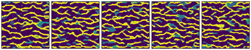
(a) $k_{\mathrm{poly,vgg}}$

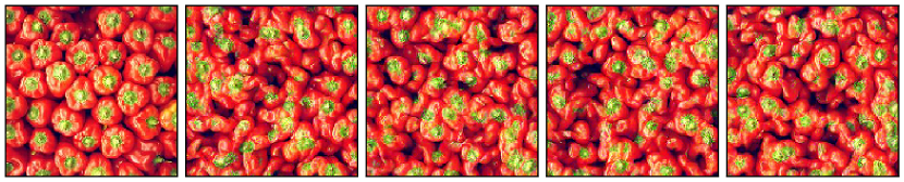
(b) $k_{\mathrm{poly,vgg}}$

Figure 7: Optimization-based synthesis using the kernel from [9], i.e. VGG encoder + polynomial kernel of second degree. Compare (a) with Figure 3(a), Figure 3(b), and Figure 4(a).

Neural generators

The present approach to train a generator is based on [49] where a sample entropy estimator based on the nearest neighbor is used. Here we use a $k^{\mathrm{th}}$ nearest neighbor [11] estimation which we found to be numerically more stable. These estimators, however, measure the distance between realizations in the raw representation, which for images may not be well suited. An ad-hoc alternative can be found in [22] where distances are instead computed on the feature responses of a neural network evaluated on the images. Other alternatives include normalizing flow [38], autoregressive flow [17], and Stein variational gradient descent [8]. The latter is an interesting alternative which involves yet another kernel to estimate the average diversity in the sample, making it useful for embedding prior knowledge about the geology.

Adaptive kernels

The kernel has a big influence on the quality of the synthesis since it defines the discriminative power of the MMD. In this work, we first reduce the data using a fixed encoder of an autoencoder previously trained on patches of the exemplar image. The same approach is employed in [23] in the context of generative modeling of natural images [5]. This is done following the intuition that distances in the code representation of an autoencoder are more suitable than in the raw pixel representation of images and spatial data. This manual kernel engineering can be circumvented by considering adaptive kernels [20]. The idea here is to iteratively update the kernel encoder during the training iterations, thus serving as an adversary maximizing the MMD whereas the generator is trained to minimize it. This idea can be taken further by considering other functions aside from kernels, e.g. parametrized by neural networks [10]. All these methods involve adversarial training of an additional neural network as well as dynamic target loss functions, involving numerical challenges in terms of stability as well as computational cost. On the upside, they tend to produce state-of-the-art results in computer vision.

6 Conclusion

We introduced a synthesis method for geological images consisting of minimizing the discrepancy in the patch distribution between an exemplar image and the synthesized image. To make the synthesis parametric and efficient, a neural network is trained in an offline phase to sample realizations quickly during deployment. We assessed the framework using the classical exemplar image by Strebelle of size $250\times 250$, and synthesize images of sizes $256\times 256$ and $512\times 512$. We find that with an adequate kernel, the visual patterns from the exemplar image are clearly reproduced, and the spatial statistics as measured by the image histogram and the two-point probability functions show good agreement with respect to the exemplar. Our framework depends on the discriminative power of the MMD, which is highly influenced by the kernel choice, as verified in our work when synthesizing using different kernels. To train the generative neural network, we currently use a sample entropy estimator based on distances in pixel space, which might not be ideal for spatial data. We discussed possible improvements to our framework such as adaptive kernels and kernel-based training of the generator. These are worth exploring in future work, as well as incorporating soft and hard conditioning.

Appendix A Implementation details

A.1 Autoencoder

The architecture of the autoencoder is designed based on the template provided in [34]: The encoder $h\colon\tilde{\mathcal{X}}\to\mathbb{R}^{8}$ is a chain of convolutions with leaky ReLU activations, with $\tanh$ activation in the last layer. The decoder $d\colon\mathbb{R}^{8}\to\tilde{\mathcal{X}}$ is a chain of transposed convolutions with ReLU activations, also with $\tanh$ in the final layer. The code size is $8$. The architecture is detailed in Table 1. We train to minimize $\operatorname*{arg\,min}_{d,h}{||x-d(h(x))||^{2}}$ on patches of the exemplar image. To reduce overfitting, we data-augment by performing horizontal and vertical flips on the patches, as well as smoothing by adding a small amount of Gaussian noise (with $0.05$ standard deviation). We use the Adam optimizer with default parameters and learning rate $10^{-3}$, and train for $2000$ iterations using a batch size of $32$. The model takes a few seconds to train using a GTX Titan X. The decoder is discarded after training and we keep the encoder for the MMD kernel.

A.2 Generator

The generator is also designed based on the template provided in [34], but we replace most of the transposed convolutions with upsampling + convolution (motivated by [30]), and add an additional convolving layer before the output. Specifically, the transposed convolutions are replaced by a $\times 2$ nearest neighbor upsampling followed by a convolution. The activation in the last layer is $\tanh$. The architecture is detailed in Table 2. We use the Adam optimizer with default parameters and learning rate $10^{-3}$, and train for $50000$ iterations for both the $256\times 256$ and $512\times 512$ generators. Using a GTX Titan X, training takes about $2.5$ and $5$ hours for sizes $256\times 256$ and $512\times 512$, respectively . In the online phase, the generators can synthesize images at the rate of approximately 150/s and 50/s for sizes $256\times 256$ and $512\times 512$, respectively.

State size	Layer
$1\times 64\times 64$	Conv(4,2,1), BN, lReLU
$32\times 32\times 32$	Conv(4,2,1), BN, lReLU
$64\times 16\times 16$	Conv(4,2,1), BN, lReLU
$128\times 8\times 8$	Conv(4,2,1), BN, lReLU
$256\times 4\times 4$	Conv(4,1,0), Tanh
$8\times 1\times 1$	–

(a) Encoder

State size	Layer
$8\times 1\times 1$	ConvT(4,1,0), BN, ReLU
$256\times 4\times 4$	ConvT(4,2,1), BN, ReLU
$128\times 8\times 8$	ConvT(4,2,1), BN, ReLU
$64\times 16\times 16$	ConvT(4,2,1), BN, ReLU
$32\times 32\times 32$	ConvT(4,2,1), Tanh
$1\times 64\times 64$	–

(b) Decoder

Table 1: Autoencoder architecture. Conv/ConvT=convolution/transposed convolution, the triplet indicates (filter size, stride, padding), BN=batch normalization.

State size	Layer
$256\times 1\times 1$	ConvT(4,1,0), BN, ReLU
$2048\times 4\times 4$	UpConv(3,1,1), BN, ReLU
$1024\times 8\times 8$	UpConv(3,1,1), BN, ReLU
$512\times 16\times 16$	UpConv(3,1,1), BN, ReLU
$256\times 32\times 32$	UpConv(3,1,1), BN, ReLU
$128\times 64\times 64$	UpConv(3,1,1), BN, ReLU
$64\times 128\times 128$	UpConv(3,1,1), BN, ReLU
$64\times 256\times 256$	Conv(3,1,1), Tanh
$1\times 256\times 256$	–

(a) $256\times 256$ generator.

State size	Layer
$512\times 1\times 1$	ConvT(4,1,0), BN, ReLU
$4096\times 4\times 4$	UpConv(3,1,1), BN, ReLU
$2048\times 8\times 8$	UpConv(3,1,1), BN, ReLU
$1024\times 16\times 16$	UpConv(3,1,1), BN, ReLU
$512\times 32\times 32$	UpConv(3,1,1), BN, ReLU
$256\times 64\times 64$	UpConv(3,1,1), BN, ReLU
$128\times 128\times 128$	UpConv(3,1,1), BN, ReLU
$64\times 256\times 256$	UpConv(3,1,1), BN, ReLU
$64\times 512\times 512$	Conv(3,1,1), Tanh
$1\times 512\times 512$	–

(b) $512\times 512$ generator.

Table 2: Generator architecture. UpConv=$\times 2$ upsample + convolution, ConvT=transposed convolution, the triplet indicates (filter size, stride, padding), BN=batch normalization.

Appendix B Additional results

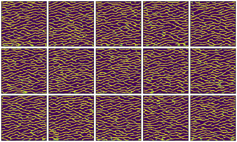
(a) Random realizations ($512\times 512$, optimization-based synthesis).

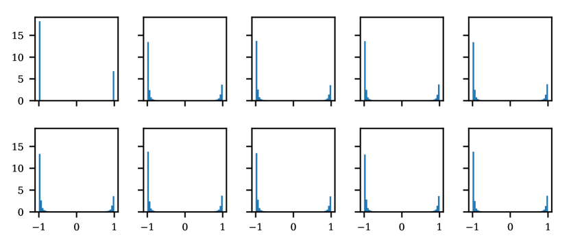
(b) Image histogram of 9 random realizations. The first histogram (top left) corresponds to the exemplar image.

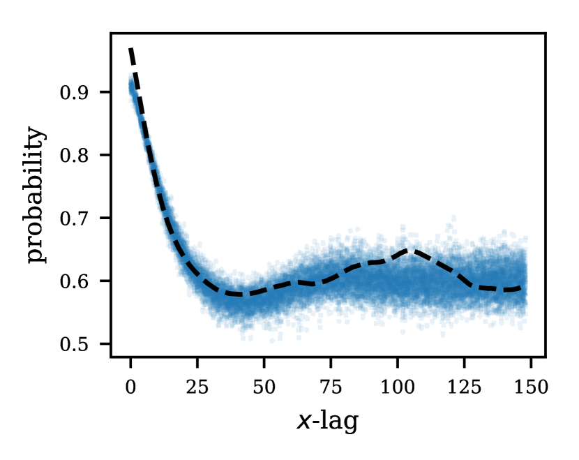
(c) Two-point probability in the $x$ direction of 100 realizations.

(d) Two-point probability in the $y$ direction of 100 realizations.

Figure 8: Results for optimization-based synthesis of realizations of size $512\times 512$ with $k_{\textrm{rq,encoder}}$ kernel.

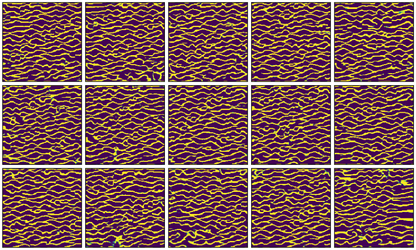
(a) Random realizations ($512\times 512$, generated by neural network).

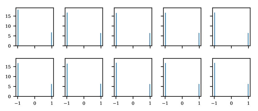
(b) Image histogram of 9 random realizations. The first histogram (top left) corresponds to the exemplar image.

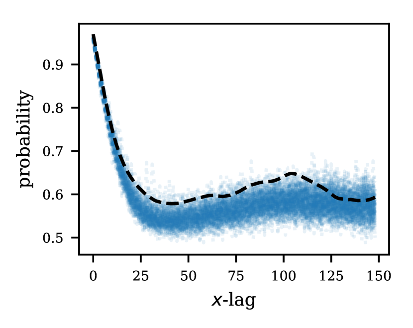
(c) Two-point probability in the $x$ direction of 100 realizations.

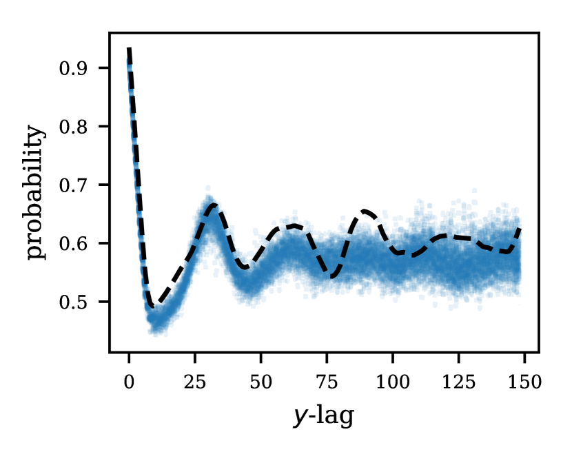
(d) Two-point probability in the $y$ direction of 100 realizations.

Figure 9: Results for neural synthesis of realizations of size $512\times 512$ with $k_{\textrm{rq,encoder}}$ kernel.

References

- Bingham and Mannila [2001] Ella Bingham and Heikki Mannila. Random projection in dimensionality reduction: applications to image and text data. In Proceedings of the seventh ACM SIGKDD international conference on Knowledge discovery and data mining, pages 245–250. ACM, 2001.
- Chan and Elsheikh [2018] Shing Chan and Ahmed H Elsheikh. Parametric generation of conditional geological realizations using generative neural networks. arXiv preprint arXiv:1807.05207, 2018.
- Chen et al. [2016] Xi Chen, Yan Duan, Rein Houthooft, John Schulman, Ilya Sutskever, and Pieter Abbeel. Infogan: Interpretable representation learning by information maximizing generative adversarial nets. In Advances in neural information processing systems, pages 2172–2180, 2016.
- Dupont et al. [2018] Emilien Dupont, Tuanfeng Zhang, Peter Tilke, Lin Liang, and William Bailey. Generating realistic geology conditioned on physical measurements with generative adversarial networks. arXiv preprint arXiv:1802.03065, 2018.
- Dziugaite et al. [2015] Gintare Karolina Dziugaite, Daniel M Roy, and Zoubin Ghahramani. Training generative neural networks via maximum mean discrepancy optimization. arXiv preprint arXiv:1505.03906, 2015.
- Efros and Freeman [2001] Alexei A Efros and William T Freeman. Image quilting for texture synthesis and transfer. In Proceedings of the 28th annual conference on Computer graphics and interactive techniques, pages 341–346. ACM, 2001.
- Efros and Leung [1999] Alexei A Efros and Thomas K Leung. Texture synthesis by non-parametric sampling. In iccv, page 1033. IEEE, 1999.
- Feng et al. [2017] Yihao Feng, Dilin Wang, and Qiang Liu. Learning to draw samples with amortized stein variational gradient descent. arXiv preprint arXiv:1707.06626, 2017.
- Gatys et al. [2015] Leon A Gatys, Alexander S Ecker, and Matthias Bethge. A neural algorithm of artistic style. arXiv preprint arXiv:1508.06576, 2015.
- Goodfellow et al. [2014] Ian Goodfellow, Jean Pouget-Abadie, Mehdi Mirza, Bing Xu, David Warde-Farley, Sherjil Ozair, Aaron Courville, and Yoshua Bengio. Generative adversarial nets. In Advances in neural information processing systems, pages 2672–2680, 2014.
- Goria et al. [2005] Mohammed Nawaz Goria, Nikolai N Leonenko, Victor V Mergel, and Pier Luigi Novi Inverardi. A new class of random vector entropy estimators and its applications in testing statistical hypotheses. Journal of Nonparametric Statistics, 17(3):277–297, 2005.
- Gretton et al. [2007] Arthur Gretton, Karsten M Borgwardt, Malte Rasch, Bernhard Schölkopf, and Alex J Smola. A kernel method for the two-sample-problem. In Advances in neural information processing systems, pages 513–520, 2007.
- Gretton et al. [2012] Arthur Gretton, Karsten M Borgwardt, Malte J Rasch, Bernhard Schölkopf, and Alexander Smola. A kernel two-sample test. Journal of Machine Learning Research, 13(Mar):723–773, 2012.
- Hinton and Salakhutdinov [2006] Geoffrey E Hinton and Ruslan R Salakhutdinov. Reducing the dimensionality of data with neural networks. science, 313(5786):504–507, 2006.
- Khaninezhad et al. [2012] Mohammadreza Mohammad Khaninezhad, Behnam Jafarpour, and Lianlin Li. Sparse geologic dictionaries for subsurface flow model calibration: Part i. inversion formulation. Advances in Water Resources, 39:106–121, 2012.
- Kingma and Ba [2014] Diederik Kingma and Jimmy Ba. Adam: A method for stochastic optimization. arXiv preprint arXiv:1412.6980, 2014.
- Kingma et al. [2016] Diederik P Kingma, Tim Salimans, Rafal Jozefowicz, Xi Chen, Ilya Sutskever, and Max Welling. Improved variational inference with inverse autoregressive flow. In Advances in Neural Information Processing Systems, pages 4743–4751, 2016.
- Kozachenko and Leonenko [1987] LF Kozachenko and Nikolai N Leonenko. Sample estimate of the entropy of a random vector. Problemy Peredachi Informatsii, 23(2):9–16, 1987.
- Laloy et al. [2017] Eric Laloy, Romain Hérault, Diederik Jacques, and Niklas Linde. Efficient training-image based geostatistical simulation and inversion using a spatial generative adversarial neural network. arXiv preprint arXiv:1708.04975, 2017.
- Li et al. [2017a] Chun-Liang Li, Wei-Cheng Chang, Yu Cheng, Yiming Yang, and Barnabás Póczos. Mmd gan: Towards deeper understanding of moment matching network. In Advances in Neural Information Processing Systems, pages 2203–2213, 2017a.
- Li et al. [2017b] Yanghao Li, Naiyan Wang, Jiaying Liu, and Xiaodi Hou. Demystifying neural style transfer. arXiv preprint arXiv:1701.01036, 2017b.
- Li et al. [2017c] Yijun Li, Chen Fang, Jimei Yang, Zhaowen Wang, Xin Lu, and Ming-Hsuan Yang. Diversified texture synthesis with feed-forward networks. In Proc. CVPR, 2017c.
- Li et al. [2015] Yujia Li, Kevin Swersky, and Rich Zemel. Generative moment matching networks. In International Conference on Machine Learning, pages 1718–1727, 2015.
- Ma and Zabaras [2011] Xiang Ma and Nicholas Zabaras. Kernel principal component analysis for stochastic input model generation. Journal of Computational Physics, 230(19):7311–7331, 2011.
- Mariethoz and Caers [2014] Gregoire Mariethoz and Jef Caers. Multiple-point geostatistics: stochastic modeling with training images. John Wiley & Sons, 2014.
- Mariethoz and Lefebvre [2014] Gregoire Mariethoz and Sylvain Lefebvre. Bridges between multiple-point geostatistics and texture synthesis: Review and guidelines for future research. Computers & Geosciences, 66:66–80, 2014.
- Mariethoz et al. [2010] Gregoire Mariethoz, Philippe Renard, and Julien Straubhaar. The direct sampling method to perform multiple-point geostatistical simulations. Water Resources Research, 46(11), 2010.
- Mosser et al. [2017] Lukas Mosser, Olivier Dubrule, and Martin J Blunt. Reconstruction of three-dimensional porous media using generative adversarial neural networks. arXiv preprint arXiv:1704.03225, 2017.
- Mosser et al. [2018] Lukas Mosser, Olivier Dubrule, and Martin J Blunt. Conditioning of three-dimensional generative adversarial networks for pore and reservoir-scale models. arXiv preprint arXiv:1802.05622, 2018.
- Odena et al. [2016] Augustus Odena, Vincent Dumoulin, and Chris Olah. Deconvolution and checkerboard artifacts. Distill, 2016. doi: 10.23915/distill.00003. URL http://distill.pub/2016/deconv-checkerboard.
- Pan and Yang [2010] Sinno Jialin Pan and Qiang Yang. A survey on transfer learning. IEEE Transactions on knowledge and data engineering, 22(10):1345–1359, 2010.
- Paszke et al. [2017] Adam Paszke, Sam Gross, Soumith Chintala, Gregory Chanan, Edward Yang, Zachary DeVito, Zeming Lin, Alban Desmaison, Luca Antiga, and Adam Lerer. Automatic differentiation in pytorch. 2017.
- Pratt [1993] Lorien Y Pratt. Discriminability-based transfer between neural networks. In Advances in neural information processing systems, pages 204–211, 1993.
- Radford et al. [2015] Alec Radford, Luke Metz, and Soumith Chintala. Unsupervised representation learning with deep convolutional generative adversarial networks. arXiv preprint arXiv:1511.06434, 2015.
- Ramdas et al. [2015] Aaditya Ramdas, Sashank Jakkam Reddi, Barnabás Póczos, Aarti Singh, and Larry A Wasserman. On the decreasing power of kernel and distance based nonparametric hypothesis tests in high dimensions. In AAAI, pages 3571–3577, 2015.
- Rasmussen [2004] Carl Edward Rasmussen. Gaussian processes in machine learning. In Advanced lectures on machine learning, pages 63–71. Springer, 2004.
- Reddi et al. [2018] Sashank J Reddi, Satyen Kale, and Sanjiv Kumar. On the convergence of adam and beyond. 2018.
- Rezende and Mohamed [2015] Danilo Jimenez Rezende and Shakir Mohamed. Variational inference with normalizing flows. arXiv preprint arXiv:1505.05770, 2015.
- Sarma et al. [2008] Pallav Sarma, Louis J Durlofsky, and Khalid Aziz. Kernel principal component analysis for efficient, differentiable parameterization of multipoint geostatistics. Mathematical Geosciences, 40(1):3–32, 2008.
- Saxe et al. [2011] Andrew M Saxe, Pang Wei Koh, Zhenghao Chen, Maneesh Bhand, Bipin Suresh, and Andrew Y Ng. On random weights and unsupervised feature learning. In ICML, pages 1089–1096, 2011.
- Sezgin and Sankur [2004] Mehmet Sezgin and Bülent Sankur. Survey over image thresholding techniques and quantitative performance evaluation. Journal of Electronic imaging, 13(1):146–166, 2004.
- Simonyan and Zisserman [2014] Karen Simonyan and Andrew Zisserman. Very deep convolutional networks for large-scale image recognition. arXiv preprint arXiv:1409.1556, 2014.
- Sriperumbudur et al. [2010] Bharath K Sriperumbudur, Arthur Gretton, Kenji Fukumizu, Bernhard Schölkopf, and Gert RG Lanckriet. Hilbert space embeddings and metrics on probability measures. Journal of Machine Learning Research, 11(Apr):1517–1561, 2010.
- Sriperumbudur et al. [2011] Bharath K Sriperumbudur, Kenji Fukumizu, and Gert RG Lanckriet. Universality, characteristic kernels and rkhs embedding of measures. Journal of Machine Learning Research, 12(Jul):2389–2410, 2011.
- Strebelle and Journel [2001] Sebastien B Strebelle and Andre G Journel. Reservoir modeling using multiple-point statistics. In SPE Annual Technical Conference and Exhibition. Society of Petroleum Engineers, 2001.
- Tahmasebi et al. [2012] Pejman Tahmasebi, Ardeshir Hezarkhani, and Muhammad Sahimi. Multiple-point geostatistical modeling based on the cross-correlation functions. Computational Geosciences, 16(3):779–797, 2012.
- Torquato and Stell [1982] S. Torquato and G. Stell. Microstructure of two‐phase random media. i. the n‐point probability functions. The Journal of Chemical Physics, 77(4):2071–2077, 1982. doi: 10.1063/1.444011.
- Ulyanov et al. [2017a] Dmitry Ulyanov, Andrea Vedaldi, and Victor Lempitsky. Deep image prior. arXiv preprint arXiv:1711.10925, 2017a.
- Ulyanov et al. [2017b] Dmitry Ulyanov, Andrea Vedaldi, and Victor Lempitsky. Improved texture networks: Maximizing quality and diversity in feed-forward stylization and texture synthesis. In Proc. CVPR, 2017b.
- Vo and Durlofsky [2014] Hai X Vo and Louis J Durlofsky. A new differentiable parameterization based on principal component analysis for the low-dimensional representation of complex geological models. Mathematical Geosciences, 46(7):775–813, 2014.
- Wu et al. [1999] Ying Nian Wu, Song Chun Zhu, and Xiuwen Liu. Equivalence of julesz and gibbs texture ensembles. In Computer Vision, 1999. The Proceedings of the Seventh IEEE International Conference on, volume 2, pages 1025–1032. IEEE, 1999.