Guaranteed Globally Optimal Planar Pose Graph and Landmark SLAM via Sparse-Bounded Sums-of-Squares Programming

Abstract

Autonomous navigation requires an accurate model or map of the environment. While dramatic progress in the prior two decades has enabled large-scale SLAM (SLAM), the majority of existing methods rely on non-linear optimization techniques to find the MLE (MLE) of the robot trajectory and surrounding environment. These methods are prone to local minima and are thus sensitive to initialization. Several recent papers have developed optimization algorithms for the Pose-Graph SLAM problem that can certify the optimality of a computed solution. Though this does not guarantee a priori that this approach generates an optimal solution, a recent extension has shown that when the noise lies within a critical threshold that the solution to the optimization algorithm is guaranteed to be optimal. To address the limitations of existing approaches, this paper illustrates that the Pose-Graph SLAM and Landmark SLAM can be formulated as polynomial optimization programs that are SOS (SOS) convex. This paper then describes how the Pose-Graph and Landmark SLAM problems can be solved to a global minimum without initialization regardless of noise level using the Sparse-BSOS (Sparse-BSOS) hierarchy. This paper also empirically illustrates that convergence happens at the second step in this hierarchy. In addition, this paper illustrates how this Sparse-BSOS hierarchy can be implemented in the complex domain and empirically shows that convergence happens also at the second step of this complex domain hierarchy. Finally, the superior performance of the proposed approach when compared to existing SLAM methods is illustrated on graphs with several hundred nodes.

I Introduction

An accurate map of the environment is essential for safe autonomous navigation in the real-world [1]. An error in the map has the potential to cause loss of life in self-driving car applications or the loss of millions/billions of dollars of assets/time resources when performing underwater or space exploration tasks. Despite the importance of accurate mapping, the majority of algorithms used for SLAM are prone to local minima and are sensitive to initialization. Troublingly, verification of these maps is either performed by visual inspection or not at all.

There has been significant recent interest in developing optimization and estimation algorithms that provide mathematical guarantees on whether a computed solution is or is close to the global optimum and is therefore true MAP (MAP) estimate of the map [2, 3, 4, 5, 6, 7]. These algorithms either use a relaxation or the dual of the original problem to find a solution. As a result these methods either return an approximate solution, are only able to certify the optimally of a solution after it has been computed, or are only able to return the global solution if the graph meets certain requirements related to limits on noise measurement. In addition, with the exception of [6], these methods are focused on pose-graph optimization and are unable to handle landmark position measurements or are unable to estimate landmark positions.

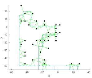
(a) Ground Truth - No Noise

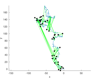
(b) Random Initialization

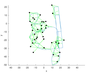
(c) Levenberg-Marquardt

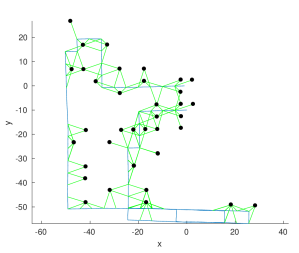
(d) SBSOS-SLAM

Figure 1: Estimated Landmark SLAM solution for the first 430 nodes(40 landmarks) of the CityTrees10000 dataset [8]. LABEL:sub@fig:1_gt shows the groundtruth pose and landmark positions before noise is added. Levenberg-Marquardt was randomly initialized and becomes trapped in a local minimum. LABEL:sub@fig:1_random_init shows the random initialization and LABEL:sub@fig:1_LM shows the LM solution. LABEL:sub@fig:1_SBSOS shows the optimal solution found by SBSOS-SLAM. Our algorithm formulates the Pose Graph and Landmark SLAM problems as SOS optimization problems which require no initializations.

In the original version of this paper, we argued in error that convergence could happen at the first step of the SBSOS hierarchy. This error arose due to a misapplication of Theorem 3 in [9]. This error was pointed out by several colleagues [10]. To address this mistake, as depicted in Figure 1d, the contributions of this paper are the following:

1. We formulate the pose graph and landmark planar SLAM as polynomial optimization programs.

2. We describe how the Sparse-BSOS hierarchy of semidefinite programs (SDP) can be used to find its solution [11, 9].

3. We empirically illustrate that convergence of the SLAM problem happens at the second step of the hierarchy

4. We show that we can formulate the Sparse-BSOS hierarchical description of the pose-graph SLAM problem as an equivalent hierarchy of sparse semidefinite programs in the complex domain. We empirically illustrate that the pose-graph SLAM problem formulated as a sparse semidefinite program hierarchy over the complex domain converges at the second step of the hierarchy.

II Related Work

SLAM refers to the problem of estimating the trajectory of a robotic vehicle over time while simultaneously estimating a model of the surrounding environment [1]. Initial algorithms used extended Kalman filter and particle filter based methods to simultaneously estimate the position of the robot and the position of observed landmarks in the environment [12, 13, 14], which we refer to as the Landmark SLAM problem. Since these methods had challenges scaling to larger datasets, researchers began applying information filter and MLE based methods which could exploit sparsity to solve larger instances of the SLAM problem. To improve the sparsity of the problem, research shifted to solving the Pose Graph SLAM problem wherein the landmarks are marginalized out and only the pose of the robot is optimized over at each time step. The majority of modern SLAM algorithms seek to find the MLE of the robot trajectory through the use of nonlinear estimation based techniques [15, 16, 8, 17]. However, the non-linear optimization algorithms used in these methods are dependent on initialization.

Several algorithms leverage theory from the field of convex optimization to overcome this dependence on initialization [18]. Optimization over the special euclidean group ($\mathrm{SE}(d)$) has generally been considered a non-convex problem and thus the majority of algorithms rely on some form of convex relaxation to estimate an approximate and sometimes exact solution to the problem. For instance the Pose Graph and Landmark SLAM problems have been formulated as a non-convex quadratically constrained quadratic program, which was then relaxed into an SDP (SDP) [7, 6]. Rosen et al. [4] relaxes optimization over the special orthogonal group ($\mathrm{SO}(d)$) to the convex hull of $\mathrm{SO}(d)$ which can be represented using convex semidefinite constraints. Since each of these methods only provide an approximate solution to the SLAM problem, they are usually only used as an initial stage and their output is then used to initialize a non-linear optimization method [8, 17].

A number of methods take advantage of Lagrangian Duality to convert the Pose Graph SLAM problem into a convex optimization problem that is equivalent to the original optimization problem if the duality gap is zero [18, Section 5.3.2]. Carlone et al. [5] uses Lagrangian Duality to develop a pair of methods to verify if a computed solution is globally optimal. Carlone et al. [3] applies a similar technique to the planar Pose Graph SLAM problem. SE-Sync proposed by Rosen et al. [2] extends this prior work and dramatically increases the scalability of the algorithm by taking advantage of a technique called the Riemannian staircase [19] that enables efficient optimization over semidefinite matrices if the solution has low-rank. These methods are only guaranteed to find the globally optimal solution if the measurement noise in the problem lies below a critical threshold and are restricted to the case of Pose Graph SLAM where factors are relative pose measurements in $\mathrm{SE}(d)$. More recently techniques have been proposed to formulate these descriptions of the Pose Graph SLAM problem in the complex domain wherein they can be solved more efficiently than similar problems formulated over the real domain [20, 21].

III Notation and Preliminaries

This section defines the notation used throughout the remainder of the paper and presents several preliminary results from the literature which are used in the paper.

Let bold lowercase letters represent vectors and blackboard bold uppercase letters represent sets. Let $i$ denote the imaginary unit and $\emptyset$ the empty set. Let $|z|=\sqrt{z_{\text{re}}^{2}+z_{\text{im}}^{2}}$ denote the magnitude of a complex number $z=z_{\text{re}}+z_{\text{im}}\cdot i$ where $z_{\text{re}}$ and $z_{\text{im}}$ give the real and imagine parts of $z$. Let $|\mathbb{A}|$ denote the cardinality of a set $\mathbb{A}$, and let $\mathbb{A}\setminus\mathbb{B}$ denote the set subtraction between sets $\mathbb{A}$ and $\mathbb{B}$. Let $\{a_{j}\}_{j}$ denote the collection of items $a_{j}$ indexed by $j$. Let $\mathbb{R}$, $\mathbb{C}$, $\mathbb{Z}$, and $\mathbb{Z}_{+}$ denote the sets of real numbers, complex numbers and integers and positive integers, respectively. Let $\|\bm{v}\|$ denote the Euclidean norm of vector $\bm{v}$. Let $\mathbb{S}_{m}\subset\mathbb{R}^{m\times m}$ denote the collection of $m$-by-$m$ symmetric real matrices. Let $\mathbb{S}^{1}\subset\mathbb{C}$ denote the circle centered at zero with radius 1 in the complex domain. Let $\mathbb{T}^{n}:=\underbrace{\mathbb{S}^{1}\times\ldots\times\mathbb{S}^{1}}_{n}\subset\mathbb{C}^{n}$ denote the torus.

Given an arbitrary matrix $A\in\mathbb{R}^{m\times m}$, let $A^{\top}$ denote its transpose, let $tr(A)$ denote its trace, let $[A]_{(j_{1},j_{2})}$ denote its $(j_{1},j_{2})$-th element, let $\text{nnz}(A)$ denote the number of nonzero elements, and let $\text{sym}(A):=\frac{1}{2}(A+A^{\top})$. Suppose $A$ is a symmetric matrix $A$, then let $A\succeq 0$ denote that the matrix is positive semi-definite and let $A\succ 0$ denote that the matrix is positive definite. Let $I_{m}$ and $0_{m}$ denote the $m$-dimensional identity and zero matrices, respectively. Let $1_{m_{1}\times m_{2}}$ denote the $m_{1}-$by$-m_{2}$ matrix with all elements being 1, and $c_{m}$ denote the $m$-by-$m$ square matrix with all elements being the constant $c$. Let $\text{diag}(A)$ denote a row vector that collects diagonal elements of matrix $A$.

IV Polynomial Optimization SLAM Formulation

This section formulates the Pose Graph and Landmark SLAM problems as polynomial optimization programs.

IV-A Polynomial Optimization

A polynomial optimization program is an optimization problem of the following form [11, Section 2.2]:

$$f^{*}=\underset{\mathbf{x}}{\operatorname{min}}\>\{f(\mathbf{x}):\mathbf{x}\in\mathbf{K}\}$$ (1)

where $f\in\mathbb{R}[\mathbf{x}]$, $\mathbb{R}[\mathbf{x}]$ is the ring of all possible polynomials in the variable $\mathbf{x}=(x_{1},\dots,x_{N})$, and $\mathbf{K}\subset\mathbb{R}^{N}$ is the semi-algebraic set

$$\mathbf{K}=\{\mathbf{x}\in\mathbb{R}^{N}:0\leq g_{j}(\mathbf{x})\leq 1,j=1,\dots,M\},$$ (2)

for polynomials $g_{j}\in\mathbb{R}[\mathbf{x}],j=1,\dots,M$.

IV-B Pose Graph SLAM

In planar Pose Graph SLAM, one estimates the pose of the robot, $(\mathbf{R}_{i},\mathbf{t}_{i})\in\mathrm{SE}(2)$ with respect to a static global reference frame at each time steps $i\in\{1,\dots,n\}$, by minimizing the error in a set of $m_{Rel}$ relative pose measurements $(\mathrm{bar}{\mathbf{R}}_{ij},\mathrm{bar}{\mathbf{t}}_{ij})\in\mathrm{SE}(2)$. The set of available measurements can be represented by the set of edges, $E=\{i_{k},j_{k}\}_{k=1}^{m_{Rel}}\subset\{1,\dots,n\}\times\{1,\dots,n\}$, in the corresponding factor graph. We denote the pose of the robot at time step $i$ by the matrix $\mathbf{H}_{i}=[\mathbf{R}_{i}|\mathbf{t}_{i}]$ and the relative pose measurement that relates the pose of the robot at time steps $i$ and $j$ by $\mathrm{bar}{\mathbf{H}}_{ij}=[\mathrm{bar}{\mathbf{R}}_{ij}|\mathrm{bar}{\mathbf{t}}_{ij}]$. We assume that each $\mathrm{bar}{\mathbf{R}}_{ij}$ and $\mathrm{bar}{\mathbf{t}}_{ij}$ are conditionally independent given the true state, that $\mathrm{bar}{\mathbf{R}}_{ij}\sim\text{Langevin}(\mathbf{R}_{ij},\omega^{2}_{\mathbf{R}_{ij}})$, and that $\mathrm{bar}{\mathbf{t}}_{ij}\sim\mathcal{N}(\mathbf{t}_{ij},\Omega_{\mathbf{t}_{ij}}^{-1})$, where $(\mathbf{R}_{ij},\mathbf{t}_{ij})$ is the true relative pose, $\omega^{2}_{\mathbf{R}_{ij}}$ is the concentration parameter of the Langevin Distribution, and $\Omega_{\mathbf{t}_{ij}}=\text{blkdiag}(\omega^{2}_{x_{ij}},\omega^{2}_{y_{ij}})$ is the information matrix of $\mathrm{bar}{\mathbf{t}}_{ij}$. Note $\text{blkdiag}(\omega^{2}_{x_{ij}},\omega^{2}_{y_{ij}})$ denotes a block diagonal matrix whose diagonal elements are equal to $\omega^{2}_{x_{ij}}$ and $\omega^{2}_{y_{ij}}$.

Under these assumptions, the MLE solution to the planar pose graph SLAM problem is equivalent to:

$$\underset{\mathbf{H}_{1},\dots,\mathbf{H}_{n}\in\mathrm{SE}(2)}{\operatorname{\text{argmin}}}\>\sum\limits_{(i,j)\in E} \omega^{2}_{\mathbf{R}_{ij}}\left|\left|\mathbf{R}_{j}-\mathbf{R}_{i}\mathrm{bar}{\mathbf{R}}_{ij}\right|\right|_{F}^{2}+$$ (3)

$$~{}~{}\left|\left|\mathbf{t}_{j}-\mathbf{t}_{i}-\mathbf{R}_{i}\mathrm{bar}{\mathbf{t}}_{ij}\right|\right|_{\Omega_{\mathbf{t}_{ij}}}^{2}$$

where $||\cdot||_{F}$ is the Frobenius norm and $||\mathbf{x}||^{2}_{\Omega}=\mathbf{x}^{\top}\Omega\mathbf{x}$ for $x\in\mathbb{R}^{2}$ [2, 22].

Note that $\mathbf{R}_{i}\in\mathrm{SO}(2)$ for each $i\in\{1,\dots,n\}$. $\mathrm{SO}(2)$ can be defined as follows:

$$\mathrm{SO}(2)=\left\{\mathbf{R}=\left[\begin{array}[]{cc}c&-s\\ s&c\end{array}\right]\in\mathbb{R}^{2\times 2}~{}\bigl{|}~{}c^{2}+s^{2}=1\right\}.$$ (6)

This definition allows us to parameterize $\mathbf{H}_{i}$ and $\mathbf{H}_{ij}$ using $(c_{i},s_{i},x_{i},y_{i})$ and $(c_{ij},s_{ij},x_{ij},y_{ij})$ respectively,

$$\mathbf{H}_{i}=\left[\begin{array}[]{ccc}c_{i}&-s_{i}&x_{i}\\ s_{i}&c_{i}&y_{i}\\ \end{array}\right],\mathbf{H}_{ij}=\left[\begin{array}[]{ccc}c_{ij}&-s_{ij}&x_{ij}\\ s_{ij}&c_{ij}&y_{ij}\\ \end{array}\right],$$ (11)

as long as we enforce that $c_{i}^{2}+s_{i}^{2}=1$. To simplify this notation, we define the sets $\mathbf{c}=\{c_{1},\dots,c_{n}\}$, $\mathbf{s}=\{s_{1},\dots,s_{n}\}$, $\mathbf{x}=\{x_{1},\dots,x_{n}\}$, and $\mathbf{y}=\{y_{1},\dots,y_{n}\}$.

If we evaluate the norms in (3) under this parameterization, then (3) is equivalent to

$$\underset{\mathbf{c},\mathbf{s},\mathbf{x},\mathbf{y}}{\operatorname{\text{argmin}}}\>\sum\limits_{(i,j)\in E}f^{\mathbf{H}}_{ij}(c_{i},s_{i},x_{i},y_{i},c_{j},s_{j},x_{j},y_{j})$$ (12)

$$~{}~{}~{}~{}~{}\text{s.t.}~{}~{}~{}c_{i}^{2}+s_{i}^{2}=1,\quad\forall i\in\{1,\dots,n\},$$

with,

$$f^{\mathbf{H}}_{ij}(c_{i}, s_{i},x_{i},y_{i},c_{j},s_{j},x_{j},y_{j})=f^{Rot}_{ij}(c_{i},s_{i},c_{j},s_{j})+$$ (13)

$$+f^{Tran}_{ij}(c_{i},s_{i},x_{i},y_{i},x_{j},y_{j}),$$

where

$$f^{Rot}_{ij}(c_{i},s_{i},c_{j},s_{j})=\omega_{\mathbf{R}_{ij}}^{2}(c_{j}-c_{i}c_{ij}+s_{i}s_{ij})^{2}+$$ (14)

$$+\omega_{\mathbf{R}_{ij}}^{2}(-s_{j}+c_{i}s_{ij}+s_{i}c_{ij})^{2}+\omega_{\mathbf{R}_{ij}}^{2}(s_{j}-s_{i}c_{ij}+$$ (15)

$$-c_{i}s_{ij})^{2}+\omega_{\mathbf{R}_{ij}}^{2}(c_{j}+s_{i}s_{ij}-c_{i}c_{ij})^{2},$$

and

$$f^{Tran}_{ij}(c_{i}, s_{i},x_{i},y_{i},x_{j},y_{j})=\omega_{x_{ij}}^{2}(x_{j}-c_{i}x_{ij}+$$ (16)

$$+s_{i}y_{ij}-x_{i})^{2}+\omega_{y_{ij}}^{2}(y_{j}-s_{i}x_{ij}-c_{i}y_{ij}-y_{i})^{2}.$$

Note that the cost is a polynomial in the space $\mathbb{R}[\mathbf{c},\mathbf{s},\mathbf{x},\mathbf{y}]$ and that each individual term $f^{\mathbf{H}}_{ij}\in\mathbb{R}[c_{i},s_{i},x_{i},y_{i},c_{j},s_{j},x_{j},y_{j}]$. We can also rewrite $c_{i}^{2}+s_{i}^{2}=1$ as $0\leq 1-c_{i}^{2}-s_{i}^{2}\leq 1$ and $0\leq 2-c_{i}^{2}-s_{i}^{2}\leq 1$ for each $i\in\{1,\ldots,n\}$. This parameterization allows us to rewrite (12) as a polynomial optimization problem in the form described in (1) and (2), where $M=2n$:

$$\underset{\mathbf{c},\mathbf{s},\mathbf{x},\mathbf{y}}{\operatorname{\text{argmin}}}\> \sum\limits_{(i,j)\in E}f^{\mathbf{H}}_{ij}(c_{i},s_{i},x_{i},y_{i},c_{j},s_{j},x_{j},y_{j})$$ (17)

s.t. $$0\leq 1-c_{i}^{2}-s_{i}^{2}\leq 1,~{}\forall i\in\{1,\dots,n\},$$

$$0\leq 2-c_{i}^{2}-s_{i}^{2}\leq 1,~{}\forall i\in\{1,\dots,n\}.$$

IV-C Landmark SLAM

In Landmark SLAM, one estimates both the pose of the robotic vehicle at each time step, $(\mathbf{R}_{i},\mathbf{t}_{i})\in\mathrm{SE}(2)$, as well as the position of observed landmarks, $\mathbf{l}_{\ell}=[l^{x}_{\ell},l^{y}_{\ell}]^{\top}\in\mathbb{R}^{2}$ for each $\ell\in\{1,\dots,w\}$, given both relative pose measurements $(\mathrm{bar}{\mathbf{R}}_{ij},\mathrm{bar}{\mathbf{t}}_{ij})\in\mathrm{SE}(2)$ and landmark position observations $\mathrm{bar}{\mathbf{l}}_{i\ell}=[x_{i\ell},y_{i\ell}]^{\top}\in\mathbb{R}^{2}$ that measure the position of landmark with respect to the local coordinate frame of the robot at the time step that it was observed. Let $L=\{i_{k},\ell_{k}\}_{k=1}^{m_{\ell}}\subset\{1,\dots,n\}\times\{1,\dots,w\}$ identify the set of landmark position measurements where $m_{\ell}$ is the number of landmark measurements and let $\mathbf{l_{x}}=\{l_{1}^{x},\dots,l_{w}^{x}\}$ and $\mathbf{l_{y}}=\{l_{1}^{y},\dots,l_{w}^{y}\}$. We assume that the relative pose measurements are distributed according to the structure defined in the previous section and that $\mathrm{bar}{\mathbf{l}}_{i\ell}\sim\mathcal{N}(\mathbf{l}^{i}_{i\ell},\Omega_{\mathbf{l}_{i\ell}}^{-1})$ where $\mathbf{l}^{i}_{i\ell}$ is the true position of the landmark $\ell$ with respect to the true pose $\mathbf{H}_{i}$ and $\Omega_{\mathbf{l}_{i\ell}}=\text{blkdiag}(\omega_{x_{i\ell}}^{2},\omega_{y_{i\ell}}^{2})$ is the information matrix of $\mathrm{bar}{\mathbf{l}}_{i\ell}$.

Under these assumptions, the MLE solution to the Landmark SLAM problem can be written as follows:

$$\underset{\mathbf{c},\mathbf{s},\mathbf{x},\mathbf{y},\mathbf{l_{x}},\mathbf{l_{y}}}{\operatorname{\text{argmin}}}\> \sum\limits_{(i,j)\in E}f^{\mathbf{H}}_{ij}(c_{i},s_{i},x_{i},y_{i},c_{j},s_{j},x_{j},y_{j})~{}+$$ (18)

$$~{}~{}~{}~{}+\sum\limits_{(i,\ell)\in L}f^{Land}_{i\ell}(c_{i},s_{i},x_{i},y_{i},l_{\ell}^{x},l_{\ell}^{y})$$

s.t. $$0\leq 1-c_{i}^{2}-s_{i}^{2}\leq 1,~{}\forall i\in\{1,\dots,n\},$$

$$0\leq 2-c_{i}^{2}-s_{i}^{2}\leq 1,~{}\forall i\in\{1,\dots,n\}.$$

with,

$$f^{Land}_{i\ell}(c_{i}, s_{i},x_{i},y_{i},l_{\ell}^{x},l_{\ell}^{y})=\omega_{x_{i\ell}}^{2}(l_{\ell}^{x}-c_{i}x_{i\ell}+$$ (19)

$$+s_{i}y_{i\ell}-x_{i})^{2}+\omega_{y_{i\ell}}^{2}(l_{\ell}^{y}-s_{i}x_{i\ell}-c_{i}y_{i\ell}-y_{i})^{2}.$$

Note that the cost of the optimization problem in (18) is a polynomial in the space $\mathbb{R}[\mathbf{c},\mathbf{s},\mathbf{x},\mathbf{y},\mathbf{l_{x}},\mathbf{l_{y}}]$ while $f^{Land}_{i\ell}\in\mathbb{R}[c_{i},s_{i},x_{i},y_{i},l_{x},l_{y}]$. Also note that the constraints are the same as in (17) and thus, (18) is a polynomial optimization problem of the form defined in (1) and (2).

V Sparse Bounded Sum-of-Squares Programming

Polynomial optimization problems in general are non-convex, however, they can be approximated and sometimes solved exactly by solving a hierarchy of convex relaxations of the problem [23]. A variety of such convex relaxations hierarchies exist. This section covers a pair of such hierarchies. The first is called the BSOS (BSOS) hierarchy and consists of a sequence of SDP relaxations that can be used to find the globally optimal solution to small polynomial optimization problems that meet certain conditions [11]. The second is called Sparse-BSOS and enables us to leverage the sparsity inherent in SLAM problems to solve larger problem sizes than is possible using BSOS [9]. We conclude the section by describing the conditions that the cost and constraints that a polynomial optimization must satisfy for the first step of either hierarchy to converge exactly to the global optimum.

V-A Bounded Sum-of-Squares

SOS programming is concerned with finding solutions to polynomial optimization problems as in (1). If $\mathbf{x}$ did not have to lie within the semi-algebraic set $\mathbf{K}$, solving the following problem would be equivalent to solving (1):

$$t^{*}=\underset{t\in\mathbb{R}}{\operatorname{sup}}\>\{t~{}|~{}f(\mathbf{x})-t\geq 0,\forall~{}\mathbf{x}\}.$$ (20)

If instead one had constraints $g_{j}$ that bound the feasible space of the variable $\mathbf{x}$ to $\mathbf{K}$, then one would need to enforce that $f(\mathbf{x})-t\geq 0,~{}\forall~{}\mathbf{x}\in\mathbf{K}$. At the same time, one would have to enforce it in a way that enabled $f-t$ to get as close to zero as possible at the optimal solution. Suppose we could optimize over a function $h$ and also strictly enforce that it be non-negative on $\mathbf{K}$. Then, by enforcing that $f(\mathbf{x})-t-h(\mathbf{x})\geq 0$, for all $x$, we would equivalently enforce that $f(\mathbf{x})-t\geq h(\mathbf{x})\geq 0$ on $\mathbf{K}$ and we would be able to optimize over $h$ to minimize the gap between $f$ and $t$ on $\mathbf{K}$.

To apply this approach using numerical optimization, one would first need to know whether it was computationally tractable to enforce positivity of $h$ on $K$. Assuming that $0\leq g_{j}(x)\leq 1$ for all $x\in\mathbf{K}$ and $\mathbf{K}$ is compact, one can prove that if a polynomial $h$ is strictly positive on $\mathbf{K}$, then $h$ can be represented as

$$h(\mathbf{x},\bm{\lambda})=\sum\limits_{\alpha,\beta\in\mathbb{N}^{M}}\lambda_{\alpha\beta}\prod_{j}\left(g_{j}(\mathbf{x})^{\alpha_{j}}(1-g_{j}(\mathbf{x}))^{\beta_{j}}\right),$$ (21)

for some (finitely many) nonnegative scalars $\bm{\lambda}=(\lambda_{\alpha\beta}$) [11, Theorem 1]. Conversely, any polynomial that can be written in the form defined in (21) is also positive on $\mathbf{K}$. This leads to a hierarchy of relaxations in which each relaxation bounds the number of monomial terms used to represent $h$ [11, Theorem 2].

Let $N^{2M}_{d}=\{(\alpha,\beta)|\alpha,\beta\in\mathbb{N}^{M},|\alpha|+|\beta|\leq d\}$ where the absolute value denotes the sum and

$$h_{d}(\mathbf{x},\bm{\lambda}):=\sum\limits_{(\alpha,\beta)\in N_{d}^{2M}}\lambda_{\alpha\beta}\prod_{j=1}^{M}g_{j}(\mathbf{x})^{\alpha_{j}}(1-g_{j}(\mathbf{x}))^{\beta_{j}},$$ (22)

where $\bm{\lambda}=(\lambda_{\alpha\beta}),(\alpha,\beta)\in\mathbb{N}^{2M}_{d}$. By choosing $d$, one can bound the number of monomial terms that are used to represent $h_{d}$ and by optimizing over $\lambda$, one can optimize over the specific polynomial. By constraining $\bm{\lambda}$ to be non-negative, one can enforce that $h_{d}$ be strictly positive on $\mathbf{K}$.

Now one can solve the following optimization problem:

$$t^{*}=\underset{t,\bm{\lambda}}{\operatorname{sup}}\{t|f(\mathbf{x})-t-h_{d}(\mathbf{x})\geq 0,\forall~{}\mathbf{x},\bm{\lambda}\geq 0\}.$$ (23)

However, optimizing over the space of all positive polynomials is computationally intractable. Instead, one can relax the problem again and optimize over the space of SOS polynomials up to a fixed degree since SOS polynomials are guaranteed to be positive and can be represented using a positive semidefinite matrix [23, Chapter 2]. Let $\Sigma[\mathbf{x}]\subset\mathbb{R}[\mathbf{x}]$ represent the space of SOS polynomials and let $\Sigma[\mathbf{x}]_{k}\subset\mathbb{R}[\mathbf{x}]_{2k}$ represent the space of SOS polynomials of degree at most $2k$. By fixing $k\in\mathbb{N}$, one arrives at the following BSOS family of convex relaxations: indexed by $d\in\mathbb{N}$:

$$q^{k}_{d}=\underset{t,\bm{\lambda}}{\operatorname{sup}}\{t|f(\mathbf{x})-t-h_{d}(\mathbf{x})\in\Sigma[\mathbf{x}]_{k},\bm{\lambda}\geq 0\}.$$ (24)

Each of these optimization programs can be implemented as an SDP and provides a lower bound on the solution to (23). Additionally, it can be shown that under certain assumptions as $d\to\infty$, $q^{k}_{d}\to f^{*}$ [11, Theorem 2]. While this is useful for small problems, as the number of variables increases or for larger values of $d$ and $k$, the runtime and memory usage of the optimization makes the use of this method infeasible [11, Section 3]. To address this challenge, we take advantage of sparsity in the optimization problem to dramatically scale problem size.

V-B Sparse Bounded Sum-of-Squares

The Sparse-BSOS hierarchy takes advantage of the fact that for many optimization problems, the variables and constraints exhibit structured sparsity. It does this by splitting the variables in the problem into $p$ blocks of variables and the cost into $p$ associated terms, such that the number of variables and constraints relevant to each block is small [9].

Given $I\subset\{1,\dots,N\}$, let $\mathbb{R}[\mathbf{x};I]$ denote the ring of polynomials in the variables $\{x_{i}:i\in I\}$. Specifically Sparse-BSOS assumes that the cost and constraints satisfy the following assumption:

Assumption 1 (Running Intersection Property (RIP)).

There exists $p\in\mathbb{N}$ and $I_{\ell}\subseteq\{1,\dots,N\}$ and $J_{\ell}\subseteq\{1,\dots,M\}$ for all $\ell\in\{1,\dots,p\}$ such that:

• $f=\sum_{\ell=1}^{p}f^{\ell}$, for some $f^{1},\dots,f^{p}$, such that
  $~{}~{}~{}f^{\ell}\in\mathbb{R}[\mathbf{x},I_{\ell}]$ for each $\ell\in\{1,\dots,p\}$,

• $g_{j}\in\mathbb{R}[\mathbf{x},I_{\ell}]$ for each $j\in J_{\ell}$ and $\ell\in\{1,\dots,p\}$,

• $\cup_{\ell=1}^{p}I_{\ell}=\{1,\dots,N\}$,

• $\cup_{\ell=1}^{p}J_{\ell}=\{1,\dots,M\}$,

• for all $\ell=1,\dots,p-1$, there is an $s\leq\ell$ such that $(I_{\ell+1}\cap\cup_{r=1}^{\ell}I_{r})\subseteq I_{s}$.

In particular, $I_{\ell}$ denotes the variables that are relevant to $\ell$-th block and $J_{\ell}$ denotes the associated relevant constraints. Intuitively, these blocks allow one to enforce positivity over a smaller set of variables which can reduce the computational burden while trying to solve this optimization problem.

We can use these definitions to define the Sparse-BSOS hierarchy that builds on the hierarchy defined in the previous section. Let $N^{\ell}:=\{(\alpha,\beta):\alpha,\beta\in\mathbb{N}_{0},\text{supp}(\alpha)\cup\text{supp}(\beta)\subseteq J_{\ell}\}$, where $\mathbb{N}_{0}$ is the set of natural numbers including $0$ and $\text{supp}(\alpha):=\{j\in\{1,\dots,M\}:\alpha_{j}\neq 0\}$. Now let $N^{\ell}_{d}:=\{(\alpha,\beta)\in N^{\ell}:\sum_{j}(\alpha_{j}+\beta_{j})\leq d\}$, with $d\in\mathbb{N}$ and let

$$h^{\ell}_{d}(\mathbf{x},\bm{\lambda}^{\ell}):=\sum\limits_{(\alpha,\beta)\in N_{d}^{\ell}}\lambda^{\ell}_{\alpha\beta}\prod_{j=1}^{M}g_{j}(\mathbf{x})^{\alpha_{j}}(1-g_{j}(\mathbf{x}))^{\beta_{j}},$$ (25)

where $\bm{\lambda}^{\ell}\in\mathbb{R}^{|N^{\ell}_{d}|}$ is the vector of scalar coefficients $\lambda_{\alpha\beta}^{\ell}$. $h^{\ell}_{d}$ is again positive on $\mathbf{K}$ as long as the elements of $\bm{\lambda}$ are positive. If we again fix $k\in\mathbb{N}$, we can define a family of optimization problems indexed by $d\in\mathbb{N}$ as shown in (26), where $d_{\max}$ is defined on page 7 of [9].

$$q^{k}_{d}=\underset{\begin{subarray}{c}t,\bm{\lambda}^{1},\dots,\bm{\lambda}^{p},\\ f^{1},\dots,f^{p}\end{subarray}}{\operatorname{sup}}\left\{t|f^{\ell}(\mathbf{x})-h^{\ell}_{d}(\mathbf{x},\bm{\lambda}^{\ell})\in\Sigma[\mathbf{x};I_{\ell}]_{k},\ell=1,\dots,p,\right.$$ (26)

$$\left.~{}~{}~{}~{}~{}~{}~{}~{}~{}~{}~{}~{}~{}~{}~{}~{}~{}~{}~{}~{}~{}~{}f(\mathbf{x})-t=\sum\limits_{\ell=1}^{p}f^{\ell}(\mathbf{x}),\bm{\lambda}^{\ell}\in\mathbb{R}^{|N_{d}^{\ell}|}\geq 0,t\in\mathbb{R},f^{\ell}\in\mathbb{R}[\mathbf{x};I_{\ell}]_{d_{max}}\right\}.$$

This hierarchy of relaxations is called the Sparse-BSOS hierarchy and each level of the hierarchy can be implemented as an SDP. In addition, if RIP is satisfied, $0\leq g_{j}(x)\leq 1$ for all $x\in\mathbf{K}$, and $\mathbf{K}$ is compact, then as $d\to\infty$, the sequence of optimization problems defined in (26) also converges to $f^{*}$[9, Theorem 2]. In addition a rank condition can be used to detect finite convergence [9, Lemma 4]. Importantly in particular cases, one can show that this optimization problem can be solved exactly when $d=1$.

VI SBSOS-SLAM

We take advantage of the Sparse-BSOS relaxation hierarchy to solve the Pose Graph and Landmark SLAM problems. In this section we talk about how we can enforce the RIP. We conclude this section with a discussion of implementation.

VI-A Satisfying the Running Intersection Property

The nature of the SLAM problem exhibits a large amount of sparsity [16, 8, 17]. However, to take advantage of the guarantees incumbent to the Sparse-BSOS hierarchy, we need to satisfy the RIP. An odometry chain forming the backbone of a SLAM graph inherently satisfies this property, however incorporating loop closures can make satisfying this assumption challenging. A better grouping increases the sparsity of the optimization problem and leads to faster solutions, but finding the optimal selection of blocks $I_{\ell}$ is NP-hard. We used the heuristic algorithm defined in [24] to generate a sequence of variable groupings for the current implementation.

VI-B Implementation and Computational Scaling

For the experiments and development presented in this paper, we modified the code base released with [9] to formulate the problem as defined earlier on in the paper. In addition, we modified the code to convert the problem to a format where we could use the SDP solver within the optimization library Mosek [25].

SOS programming optimizes over polynomials which can become ill-conditioned when optimization occurs over a large domain [9, Section 4]. Data can be scaled to address this problem, however if the optimization problem still remains poorly scaled then the optimization solver will warn the user that the problem cannot be satisfactorily solved.

VII Formulating the Rotational Averaging Problem as a sparse SDP in the Complex Domain

This section begins by describing how to formulate the Pose Graph problem without translation in the complex domain as an SDP and illustrates that it satisfies the RIP sparsity structure. We then illustrate how this complex domain SDP can be formulated as a smaller, sparse complex domain SDP that can be more readily solved.

VII-A Rotational Averaging Problem and RIP

In this manuscript we aim for solving the $n$-pose Rotational Averaging Problem

$$\inf_{\bm{c},\bm{s}\in\mathbb{R}^{n}}\quad f(\bm{c,s})\hskip 85.35826pt\texttt{(RAP)}$$

s.t. $$c_{j}^{2}+s_{j}^{2}=1,~{}~{}\forall j=1,2,\cdots,n$$

where $\bm{c}=[c_{1},\cdots,c_{n}]^{\top}$ and $\bm{s}=[s_{1},\cdots,s_{n}]^{\top}$. For simplicity define $\mathcal{C}:=\{(\bm{c,s})\mid c_{j}^{2}+s_{j}^{2}=1,~{}\forall j=1,2,\cdots,n\}\subset\mathbb{R}^{2n}$ the feasible set of (RAP). The rotational averaging cost reads

$$f(\bm{c,s})= \sum_{(j_{1},j_{2})\in\mathbb{E}}\big{(}2\Omega_{j_{1}j_{2}}^{2}(c_{j_{2}}-c_{j_{1}}c_{j_{1}j_{2}}+s_{j_{1}}s_{j_{1}j_{2}})^{2}+$$

$$\hskip 31.2982pt+2\Omega_{j_{1}j_{2}}^{2}(s_{j_{2}}-s_{j_{1}}c_{j_{1}j_{2}}-c_{j_{1}}s_{j_{1}j_{2}})^{2}\big{)}$$ (27)

$$= \sum_{(j_{1},j_{2})\in\mathbb{E}}f^{\text{rot}}_{j_{1}j_{2}}(c_{j_{1}},s_{j_{1}},c_{j_{2}},c_{j_{2}})$$ (28)

where $\mathbb{E}\subset\{1,\cdots,n\}\times\{1,\cdots,n\}$ is the collection of edges in the pose graph, $\{\Omega_{j_{1}j_{2}}\}_{(j_{1},j_{2})\in\mathbb{E}}$ is the set of concentration parameters of the Langevin Distribution, and constants $c_{j_{1}j_{2}}$ and $s_{j_{1}j_{2}}$ satisfy $c_{j_{1}j_{2}}^{2}+s_{j_{1}j_{2}}^{2}=1$ for all $(j_{1},j_{2})\in\mathbb{E}$.

Let $\mathbb{R}[(\bm{c,s})]$ denote the ring of real polynomials over $\bm{c}$ and $\bm{s}$. Given $\mathcal{I}\subseteq\{1,2,\cdots,n\}$, let $\mathbb{R}[(\bm{c,s});\mathcal{I}]$ denote the ring of polynomials in variables $\{c_{\texttt{i}}:\texttt{i}\in\mathcal{I}\}$ and $\{s_{\texttt{i}}:\texttt{i}\in\mathcal{I}\}$. Using the edges of the pose graph, one can show that the rotational averaging cost satisfies a specific sparsity structure similar as in [9, Assumption 1]:

Assumption 2.

There exists $p\in\mathbb{Z}_{+}$ and $\mathcal{I}_{\ell}\subseteq\{1,2,\cdots,n\}$ for all $\ell\in\{1,2,\cdots,p\}$ such that:

• There exists $f^{1}(\cdot),\ldots,f^{p}(\cdot)$ with $f^{\ell}(\cdot)\in\mathbb{R}[(\bm{c,s});\mathcal{I}_{\ell}]$ for each $\ell\in\{1,2,\cdots,p\}$ such that $f(\cdot)=\sum_{\ell=1}^{p}f^{\ell}(\cdot)$,

• $\cup_{\ell=1}^{p}\mathcal{I}_{\ell}=\{1,2,\cdots,n\}$,

• for each $\ell\in\{1,2,\cdots,p-1\}$, there exists an $\ell_{0}\leq\ell$ such that $(\mathcal{I}_{\ell+1}\cap\cup_{\ell_{1}=1}^{\ell}\mathcal{I}_{\ell_{1}})\subseteq\mathcal{I}_{\ell_{0}}$ (Running Intersection Property).

Note, we do not need to assume index set $\mathcal{J}_{\ell}$ over constraints as in [9, Assumption 1] because we can simply set $\mathcal{J}_{\ell}=\mathcal{I}_{\ell}$ for all $\ell$ due to the fact that every constraint in (RAP) depends on only one pose.

VII-B Formulating the Rotational Averaging Problem in the Complex Domain

For each $j\in\{1,\cdots,n\}$, let the pair $(c_{j},s_{j})$ represent the pair of $\sin(\omega_{j})$ and $\cos(\omega_{j})$ for some angle $\omega_{j}$, i.e.

$$c_{j}=\frac{e^{i\omega_{j}}+e^{-i\omega_{j}}}{2}\hskip 14.22636pt~{}s_{j}=\frac{e^{i\omega_{j}}-e^{-i\omega_{j}}}{2i}.$$ (29)

Equivalently one can let

$$c_{j}=\frac{z_{j}+z_{j}^{-1}}{2}\hskip 14.22636pt~{}s_{j}=\frac{z_{j}-z_{j}^{-1}}{2i}$$ (30)

for some complex number $z_{j}\in\mathbb{C}$ such that $|z_{j}|=1$. Let $\nu\in\mathbb{R}$ denote an arbitrary value that is strictly smaller than the minimum value $\nu^{*}\in\mathbb{R}$ of $f(\bm{c,s})$ over $\mathcal{C}$. Then $f(\bm{c,s})-\nu>0$ over $\mathcal{C}$, and we can transfer $f(\bm{c,s})-\nu$ into the complex domain via (30) to create a Laurent polynomial [26, Section 1.1] $R$ as:

$$R(\bm{z})=\sum_{\bm{k}\in\mathbb{K}}r_{\bm{k}}\bm{z^{k}}$$ (31)

with $|z_{j}|=1$ for all $j\in\{1,\ldots,n\}$ where $\bm{z}=[z_{1},\cdots,z_{n}]^{\top}\in\mathbb{C}^{n}$ and $\bm{k}=[k_{1}\cdots,k_{n}]^{\top}\in\mathbb{K}\subset\mathbb{Z}^{n}$. We postpone the specification of how $\mathbb{K}$ is decided to the next subsection, and the following lemma holds.

Lemma 3.

If $R(\bm{z})>0$ for all $\bm{z}\in\mathbb{T}^{n}$, then the constant term $r_{\bm{0}}$ of $R$ is real and strictly positive.

Proof.

To prove this result, we first describe how to transform $f(\bm{c,s})$ into $R(\bm{z})$. Then we identify a correspondence between $r_{\bm{0}}$ and the Inverse Z-Transform of $R$. We use this correspondence to prove the desired result.

Expanding $f^{\text{rot}}_{j_{1}j_{2}}(\cdot)$ we get

$$f^{\text{rot}}_{j_{1}j_{2}}(c_{j_{1}},s_{j_{1}},c_{j_{2}},c_{j_{2}})= 2\Omega_{j_{1}j_{2}}^{2}\big{(}c_{j_{1}}^{2}-2c_{j_{1}j_{2}}c_{j_{1}}c_{j_{2}}+c_{j_{2}}^{2}+$$

$$-2s_{j_{1}j_{2}}c_{j_{1}}s_{j_{2}}+2s_{j_{1}j_{2}}c_{j_{2}}s_{j_{1}}+$$

$$+s_{j_{1}}^{2}-2c_{j_{1}j_{2}}s_{j_{1}}s_{j_{2}}+s_{j_{2}}^{2}\big{)}.$$ (32)

Applying (30), $f^{\text{rot}}_{j_{1}j_{2}}$ transforms into

$$R^{\text{rot}}_{j_{1}j_{2}}(z_{j_{1}},z_{j_{2}})= 2\Omega_{j_{1}j_{2}}^{2}\big{(}2+(-c_{j_{1}j_{2}}+s_{j_{1}j_{2}}\cdot i)z_{j_{1}}^{-1}z_{j_{2}}+$$

$$+(-c_{j_{1}j_{2}}-s_{j_{1}j_{2}}\cdot i)z_{j_{1}}z_{j_{2}}^{-1}\big{)},$$ (33)

in which a constant $4\Omega_{j_{1}j_{2}}^{2}$ appears. Then since $R(\bm{z})=\sum_{(j_{1},j_{2})\in\mathbb{E}}R_{j_{1}j_{2}}^{\text{rot}}(z_{j_{1}},z_{j_{2}})-\nu$, $r_{\bm{0}}=4\sum_{(j_{1},j_{2})\in\mathbb{E}}\Omega_{j_{1}j_{2}}^{2}-\nu$ as a real number.

Notice $R$ can be seen as the $n$-dimensional $z$-transform of the sequence $\{r_{\bm{k}}\}_{\bm{k}}$ over $\mathbb{T}^{n}$ according to [27, Def. 2.1.1]. Pick a scalar $\epsilon>0$ small enough such that $R(\bm{z})>\epsilon>0$ for all $z\in\mathbb{T}^{n}$, then based on [27, Thm. 2.1.5] we have

$$r_{\bm{0}} =\frac{1}{(2\pi i)^{n}}\int_{\mathbb{T}^{n}}R(\bm{z})z_{1}^{-1}z_{2}^{-1}\cdots z_{n}^{-1}d\bm{z}$$ (34)

$$>\frac{1}{(2\pi i)^{n}}\int_{\mathbb{T}^{n}}\epsilon z_{1}^{-1}z_{2}^{-1}\cdots z_{n}^{-1}d\bm{z}$$ (35)

$$=\frac{\epsilon}{(2\pi i)^{n}}\oint_{\mathbb{S}^{1}}\cdots\oint_{\mathbb{S}^{1}}z_{1}^{-1}\cdots z_{n}^{-1}dz_{1}\cdots dz_{n}$$ (36)

$$=\frac{\epsilon}{(2\pi i)^{n}}\cdot\left(\prod_{j=1}^{n}\oint_{\mathbb{S}^{1}}z_{j}^{-1}dz_{j}\right)$$ (37)

$$=\frac{\epsilon}{(2\pi i)^{n}}\cdot\left(\prod_{j=1}^{n}2\pi i\right)$$ (38)

$$=\epsilon>0.$$ (39)

∎

Proposition 4.

The indices $\bm{k}\in\mathbb{K}$ of the non-zero coefficients of $R$ satisfy the following properties:

1. $\sum_{j=1}^{n}k_{j}=0$;

2. $-1\leq k_{j}\leq 1$ for all $j\in\{1,\cdots,n\}$;

3. if $\bm{k}$ is not the 0 vector, then only 2 component of $\bm{k}$ are nonzero;

4. for each $\bm{k}\in\mathbb{K}$, $r_{\bm{k}}=r_{\bm{-k}}^{\dagger}$ where ^† denotes the complex conjugate.

Proof.

The statement follows directly from (VII-B) and the fact that $R(\bm{z})=\sum_{(j_{1},j_{2})\in\mathbb{E}}R_{j_{1}j_{2}}^{\text{rot}}(z_{j_{1}},z_{j_{2}})-\nu$. ∎

VII-C Factorization and SDP

In this subsection we factorize $R(\bm{z})$ while preserving the sparsity structure as in Assumption 2. For each $\ell\in\{1,\ldots,p\}$, let $\phi_{\ell}(\bm{z})$ denote the column vector that stores the constant 1, every $z_{\texttt{i}}$, and every $z_{\texttt{i}_{1}}z_{\texttt{i}_{2}}$ where $\texttt{i},\texttt{i}_{1},\texttt{i}_{2}\in\mathcal{I}_{\ell}$ and $\texttt{i}_{1}\neq\texttt{i}_{2}$. Therefore $\phi_{\ell}(\bm{z})$ contains $\varrho_{\ell}:=1+|\mathcal{I}_{\ell}|+\binom{|\mathcal{I}_{\ell}|}{2}$ elements. Let $\phi(\bm{z}):=[\phi_{1}^{\top}(\bm{z}),\phi_{2}^{\top}(\bm{z}),\cdots,\phi_{p}^{\top}(\bm{z})]^{\top}$ which stacks all elements in $\phi_{\ell}(\bm{z})$ for all $\ell$, thus it contains $\varrho:=\sum_{\ell=1}^{p}\varrho_{\ell}$ elements. Let $\{\bm{k}_{j}\}_{j}$ be a sequence of $\bm{k}_{j}$ as the degree of $[\phi(\bm{z})]_{(j,1)}$ in $\bm{z}$ for all $j=1,\cdots\varrho$, thus $\{-\bm{k}_{j}\}_{j}$ collects the orders of elements in $\phi^{\dagger}(\bm{z})$. Notice that $\phi(\bm{z})$ may contain repeated elements. In addition, note $\Phi(\bm{z}):=\phi(\bm{z})\cdot\phi^{\dagger}(\bm{z})\in\mathbb{C}^{\varrho\times\varrho}$ contains all terms that appear in $R(\bm{z})$, thus for the rest of this manuscript $\mathbb{K}$ is set to be the collection of degrees of all elements in $\Phi(\bm{z})$ for clarity.

For arbitrary $\bm{k}\in\mathbb{K}$, define a binary matrix $\Theta_{\bm{k}}\in\mathbb{R}^{\varrho\times\varrho}$ that is zero everywhere except $[\Theta_{\bm{k}}]_{(j_{1},j_{2})}=1$ whenever $\bm{k}_{j_{2}}-\bm{k}_{j_{1}}=\bm{k}$, thus $tr(\Theta_{\bm{k}}\cdot\Phi(\bm{z}))=\text{nnz}(\Theta_{\bm{k}})\cdot\bm{z^{k}}$. We then introduce the following 2 lemmas that can be used to check the positivity of $R$ using $\Theta_{\bm{k}}$ and $\Phi$.

Lemma 5.

If there exists a matrix $Q\in\mathbb{C}^{\varrho\times\varrho}$ such that $r_{\bm{k}}=tr(\Theta_{\bm{k}}\cdot Q)$ holds for each $\bm{k}\in\mathbb{K}$, then $R(\bm{z})=tr(\Phi(\bm{z})\cdot Q)$.

Proof.

Notice $\Phi(\bm{z})=\sum_{\bm{k}\in\mathbb{K}}\Theta_{\bm{k}}\bm{z^{k}}$, then

$$R(\bm{z}) =\sum_{\bm{k}\in\mathbb{K}}r_{\bm{k}}\bm{z^{k}}=\sum_{\bm{k}\in\mathbb{K}}tr(\Theta_{\bm{k}}\cdot Q)\bm{z^{k}}$$ (40)

$$=tr(\sum_{\bm{k}\in\mathbb{K}}\Theta_{\bm{k}}\bm{z^{k}}\cdot Q)=tr(\Phi(\bm{z})\cdot Q)$$ (41)

in which the third equality comes from the facts that $\bm{z}^{\bm{k}}$ is a scalar and that $tr(\cdot)$ is a linear operator. ∎

Lemma 6.

If $R(\bm{z})=tr(\Phi(\bm{z})\cdot Q)$ for a $Q\in\mathbb{C}^{\varrho\times\varrho}$ that is positive semi-definite, then $f(\bm{c,s})-\nu\geq 0$ over $\mathcal{C}$.

Proof.

If $Q\succeq 0$, then $Q=Y^{*}Y$ for some complex matrix $Y$ of proper size [28, Corollary 7.2.9]. Therefore

$$R(\bm{z}) =tr(\phi(\bm{z})\phi^{\dagger}(\bm{z})\cdot Y^{*}Y)$$ (42)

$$=tr(\phi^{\dagger}(\bm{z})Y^{\dagger}Y\phi(\bm{z}))$$ (43)

$$=\phi^{\dagger}(\bm{z})Y^{\dagger}Y\phi(\bm{z})$$ (44)

$$=\|Y\phi(\bm{z})\|_{2}^{2}$$ (45)

which is non-negative for all $\bm{z}$. Since $R(\bm{z})$ is equivalent to $f(\bm{c,s})-\nu$ for $\bm{z}\in\mathbb{T}^{n}$ and $c_{i}^{2}+s_{i}^{2}=1$ for all $i\in\{1,\ldots,n\}$, then $f(\bm{c,s})-\nu\geq 0$ where $c_{i}^{2}+s_{i}^{2}=1$ for all $i\in\{1,\ldots,n\}$. ∎

One can determine whether a complex-valued matrix $Q$ is positive by checking the positivity of an equivalent real-valued matrix:

Lemma 7 (Eq. (6.26) in [29]).

Let $Q=Q_{r}+i\cdot Q_{i}$ be a complex-valued matrix where $Q_{r}$ and $Q_{i}$ represent the real and imaginary parts of $Q$. If $Q$ is Hermitian, i.e. $Q_{r}$ is symmetric and $Q_{i}$ is skew-symmetric, then

$$Q\succeq 0\iff\begin{bmatrix}Q_{r}&-Q_{i}\\ Q_{i}&Q_{r}\end{bmatrix}\succeq 0.$$ (46)

Given the two Lemmas presented above, we then seek to find a matrix $Q$ that is Hermitian and satisfies $r_{\bm{k}}=tr(\Theta_{\bm{k}}\cdot Q)$ for each $\bm{k}\in\mathbb{K}$. Notice $Q$ being Hermitian is viable since $\bm{r_{k}}=\bm{r_{-k}}^{*}$ for all $\bm{k}\in\mathbb{K}$ as stated in Lemma 4. In addition, $Q$ is also expected to be block-diagonal as in (47) in order to be compatible with the sparsity structure imposed by $\phi(\bm{z})$:

$$Q=\begin{bmatrix}Q_{1}&&&\\ &Q_{2}&&\\ &&\ddots&\\ &&&Q_{p}\end{bmatrix}\in\mathbb{C}^{\varrho\times\varrho}$$ (47)

where $Q_{\ell}\in\mathbb{C}^{\varrho_{\ell}\times\varrho_{\ell}}$ for all $\ell\in\{1,\cdots,p\}$.

To find Q and the optimal $\nu$, we can solve the following optimization

$$\sup_{Q,\nu}\quad \nu\hskip 85.35826pt\texttt{(Opt)}$$

s.t. $$tr(\Theta_{\bm{k}}\cdot Q)=r_{\bm{k}},~{}\forall\bm{k}\in\mathbb{K}$$

$$Q\text{ is Hermitian, }Q\succeq 0$$

where $\lambda\in\mathbb{R}$ is a slack variable. To formulate this problem over real-valued matrices, define a symmetric block matrix

$$X=\begin{bmatrix}Q_{r}&-Q_{i}\\ Q_{i}&Q_{r}\end{bmatrix},$$ (48)

then (Opt) can be written as an equivalent Semi-Definite Program (SDP) as in [30, eq. (1.1.1)]:

$$\inf_{X,\nu}\quad -\nu\hskip 113.81102pt\texttt{(P)}$$

s.t. $$tr(A_{m}\cdot X)=b_{m},~{}\forall m=1,2,\cdots,M$$

$$X\succeq 0$$

$$X\in\mathbb{S}_{2\varrho}$$

in which $X\succeq 0$ ensures that $Q\succeq 0$ based on Lemma 7. The cost function of (P) actually tries to maximize $\nu$, and the equality constraints in (P) enforce (47), (48), and $r_{\bm{k}}=tr(\Theta_{\bm{k}}\cdot Q)$ for all $\bm{k}\in\mathbb{K}$. In particular, the equality constraints in (P) are enforcing:

1. Block Diagonal: To ensure $Q$, or equivalently $Q_{r}$ and $Q_{i}$, are block diagonal as in (47), define

   $$Q^{\text{BD}}=\begin{bmatrix}1_{\varrho_{1}}&&&\\ &1_{\varrho_{2}}&&\\ &&\ddots&\\ &&&1_{\varrho_{p}}\end{bmatrix},$$ (49)

   $\Gamma_{1}:=\{(\gamma_{1},\gamma_{2})\in\mathbb{Z}_{+}\mid[Q^{\text{BD}}]_{(\gamma_{1}\gamma_{2})}=0,1\leq\gamma_{1}<\gamma_{2}\leq\varrho\}$, $\Gamma_{2}:=\{(\gamma_{1},\gamma_{2}+\varrho)\in\mathbb{Z}_{+}\mid[Q^{\text{BD}}]_{(\gamma_{1}\gamma_{2})}=0,1\leq\gamma_{1}<\gamma_{2}\leq\varrho\}$, and $\Gamma:=\Gamma_{1}\cup\Gamma_{2}$. For each $\gamma\in\Gamma$, define $b_{\gamma}^{\text{BD}}=0$ and $A_{\gamma}^{\text{BD}}\in\mathbb{R}^{2\varrho\times 2\varrho}$ that is 0 anywhere except $[A_{\gamma}^{\text{BD}}]_{\gamma}=1$. Then given skew symmetric $Q_{i}$, $Q_{r}$ and $Q_{i}$ are both block diagonal if $tr(\text{sym}(A_{\gamma}^{\text{BD}})\cdot X)=b_{\gamma}^{\text{BD}}$ holds for all $\gamma\in\Gamma$. Since $Q^{\text{BD}}$ is symmetric, it is easy to check $|\Gamma_{1}|=|\Gamma_{2}|=0.5(\varrho^{2}-\sum_{\ell=1}^{p}\varrho_{\ell}^{2})$ and $\Gamma_{1}\cap\Gamma_{2}=\emptyset$. Therefore in total we have $\varrho^{2}-\sum_{\ell=1}^{p}\varrho_{\ell}^{2}$ such constraints.

2. Block Matching: In $X$ we need its diagonal blocks appearing as $Q_{r}$ in (48) to be identical to one another. This condition can be enforced by defining $b_{\alpha_{1}\alpha_{2}}^{\text{BM}}=0$ and $A_{\alpha_{1}\alpha_{2}}^{\text{BM}}\in\mathbb{R}^{2\varrho\times 2\varrho}$ which is 0 everywhere except

   $$[A_{\alpha_{1}\alpha_{2}}^{\text{BM}}]_{(\alpha_{1},\alpha_{2})}=-[A_{\alpha_{1}\alpha_{2}}^{\text{BM}}]_{(\alpha_{1}+\varrho,\alpha_{2}+\varrho)}=1$$ (50)

   for all $\alpha_{1},\alpha_{2}\in\{1,2,\cdots,\varrho\}$. Therefore $tr(\text{sym}(A_{\alpha_{1}\alpha_{2}}^{\text{BM}})\cdot X)=b_{\alpha_{1}\alpha_{2}}^{\text{BM}}$ guarantees that the $(\alpha_{1}\alpha_{2})$-th elements of the first and second diagonal blocks in $X$ are the same. Because $X$ is symmetric, we have $1+2+\cdots+\varrho=0.5(\varrho^{2}+\varrho)$ such constraints.

3. Skew Symmetry: To ensure $[Q_{i}]_{(\beta_{1},\beta_{2})}=-[Q_{i}]_{(\beta_{2},\beta_{1})}$ for all indices $\beta_{1},\beta_{2}\in\{1,2,\cdots,\varrho\}$, we define the following constraints:

   $$tr(\text{sym}(A_{\beta_{1}\beta_{2}}^{\text{SS}})\cdot X)=b_{\beta_{1}\beta_{2}}^{\text{SS}}$$ (51)

   where $b_{\beta_{1}\beta_{2}}^{\text{SS}}=0$ and $A_{\beta_{1}\beta_{2}}^{\text{SS}}\in\mathbb{R}^{2\varrho\times 2\varrho}$ is 0 everywhere except

   • $[A_{\beta_{1}\beta_{2}}^{\text{SS}}]_{(\beta_{1},\beta_{2}+\varrho)}=1$ if $\beta_{1}=\beta_{2}$;

   • $[A_{\beta_{1}\beta_{2}}^{\text{SS}}]_{(\beta_{1},\beta_{2}+\varrho)}=[A_{\beta_{1}\beta_{2}}^{\text{SS}}]_{(\beta_{2},\beta_{1}+\varrho)}=1$ if $\beta_{1}\neq\beta_{2}$.

   The number of such constraints is $\varrho+\big{(}1+2+\cdots+(\varrho-1)\big{)}=0.5(\varrho^{2}+\varrho)$, where the first $\varrho$ comes from the cases when $\beta_{1}=\beta_{2}$ and the remainder of the summation comes from cases when $\beta_{1}\neq\beta_{2}$.

4. Term Matching: To ensure $r_{\bm{k}}=tr(\Theta_{\bm{k}}\cdot Q)$ for all $\bm{k}\in\mathbb{K}$, enforce the following constraints:

   $$tr(\text{sym}(A_{\bm{k}}^{\text{TMre}})\cdot X)=b_{\bm{k}}^{\text{TMre}}$$ (52)

   $$tr(\text{sym}(A_{\bm{k}}^{\text{TMim}})\cdot X)=b_{\bm{k}}^{\text{TMim}}$$ (53)

   where

   $$A_{\bm{k}}^{\text{TMre}}=\begin{bmatrix}\Theta_{\bm{k}}&\\ &0_{\varrho}\end{bmatrix}, ~{}b_{\bm{k}}^{\text{TMre}}=\text{real}(r_{\bm{k}}),$$ (54)

   $$A_{\bm{k}}^{\text{TMim}}=\begin{bmatrix}0_{\varrho}&\Theta_{\bm{k}}\\ &0_{\varrho}\end{bmatrix}, ~{}b_{\bm{k}}^{\text{TMim}}=\text{im}(r_{\bm{k}}).$$ (55)

   In total, there are $2|\mathbb{K}|$ such constraints.

Notice the second and third categories of constraints ensure that $X$ has the structure of (48). Let $\{b_{m}\}_{m}$ be the collection of all possible $b_{\gamma}^{\text{BD}}$, $b_{\alpha_{1}\alpha_{2}}^{\text{BM}}$, $b_{\beta_{1}\beta_{2}}^{\text{SS}}$, $b_{\bm{k}}^{\text{TMre}}$ and $b_{\bm{k}}^{\text{TMim}}$; let $\{A_{m}\}_{m}$ be the collection of all possible $\text{sym}(A_{\gamma}^{\text{BD}})$, $\text{sym}(A_{\alpha_{1}\alpha_{2}}^{\text{BM}})$, $\text{sym}(A_{\beta_{1}\beta_{2}}^{\text{SS}})$, $\text{sym}(A_{\bm{k}}^{\text{TMre}})$ and $\text{sym}(A_{\bm{k}}^{\text{TMim}})$. Then in total (P) has $M=2\varrho^{2}+\varrho-\sum_{\ell=1}^{p}\varrho_{\ell}^{2}+2|\mathbb{K}|$ equality constraints.

VII-D Sparse SDP

This section describes how to formulate (P) as a smaller semidefinite program by utilizing the sparsity of the problem formulation. We refer to this smaller semidefinite program as the Complex-domain SDP (CSDP).

Notice $X\in\mathbb{S}_{2\varrho}$ in (P) is indeed sparse when $p$ is large, or equivalently each $\varrho_{\ell}$ is much smaller than $\varrho$. This can be seen by comparing the size of $Q$ against the sizes of all $Q_{\ell}$ in (47). In other words, $\varrho^{2}=(\sum_{\ell=1}^{p}\varrho_{\ell})^{2}$ is much larger than $\sum_{\ell=1}^{p}\varrho_{\ell}^{2}$ when $p$ is large. We then can simplify (P) into an SDP with smaller size by transferring $X$ into a block diagonal matrix using the block diagonal structure in $Q$.

To block diagonalize $X$, for arbitrary $\varepsilon:=(\varepsilon_{1},\varepsilon_{2})\in\{1,2,\cdots,2\varrho\}^{2}$, denote $E_{\varepsilon}$ the matrix generated by exchanging the $\varepsilon_{1}$-th and $\varepsilon_{2}$-th columns of $I_{2\varrho}$. Notice $E_{\varepsilon}E_{\varepsilon}^{\top}=E_{\varepsilon}^{\top}E_{\varepsilon}=I_{2\varrho}$, and $E_{\varepsilon}=I_{2\varrho}$ if $\varepsilon_{1}=\varepsilon_{2}$. Define a linear operator $\mathfrak{E}_{\varepsilon}:\mathbb{S}_{2\varrho}\rightarrow\mathbb{S}_{2\varrho}$ as

$$\mathfrak{E}_{\varepsilon}(A)=E_{\varepsilon}^{\top}AE_{\varepsilon}$$ (56)

that switch the $\varepsilon_{1}$-th row and column with the $\varepsilon_{2}$-th row and column of $A$. Then for an subset $\mathcal{E}:=\{\varepsilon^{\mu}\}_{\mu}\subset\{1,2,\cdots,2\varrho\}^{2}$, define

$$\mathfrak{E}_{\mathcal{E}}:=\mathfrak{E}_{\varepsilon^{|\mathcal{E}|}}\circ\mathfrak{E}_{\varepsilon^{|\mathcal{E}|-1}}\circ\cdots\circ\mathfrak{E}_{\varepsilon^{1}},$$ (57)

and the following lemma holds.

Lemma 8.

$\mathfrak{E}_{\mathcal{E}}(A)$ shares the same eigenvalues with $A$ for arbitrary matrix $A\in\mathbb{S}_{2\varrho}$ and arbitrary sequence $\mathcal{E}\subset\{1,2,\cdots,2\varrho\}^{2}$.

Proof.

Due to [31, Corollary 3.3.1], symmetric matrix $A$ can be diagonalized as $A=V^{\top}\Lambda V$ where $V$ is orthogonal, i.e. $VV^{\top}=V^{\top}V=I_{2\varrho}$ and $\Lambda$ is a diagonal matrix. Notice the diagonal of $\Lambda$ collects all eigenvalues of $A$. Then for arbitrary $\varepsilon\in\{1,2,\cdots,2\varrho\}^{2}$,

$$\mathfrak{E}_{\varepsilon}(A)=E_{\varepsilon}^{\top}AE_{\varepsilon}=E_{\varepsilon}^{\top}V^{\top}\Lambda VE_{\varepsilon}=(VE_{\varepsilon})^{\top}\Lambda(VE_{\varepsilon}),$$ (58)

thus $\mathfrak{E}_{\varepsilon}(A)$ shares the same eigenvalues with $A$. The claim then follows by iterativly applying the above computation $|\mathcal{E}|$ times. ∎

Before presenting a lemma and a corollary that can be useful block diagonalze $X$, we introduce one more notation. Given an arbitrary matrix $A\in\mathbb{S}_{2\varrho}$ whose diagonal elements are all elements in $\{1,2,\cdots,p\}$, define

$$\mathbb{L}_{\ell}(A):=\begin{bmatrix}[A]_{(j_{1},j_{1})}&[A]_{(j_{1},j_{2})}&\cdots&[A]_{(j_{1},j_{l})}\\ [A]_{(j_{2},j_{1})}&[A]_{(j_{2},j_{2})}&\cdots&[A]_{(j_{2},j_{l})}\\ \vdots&\vdots&\vdots&\vdots\\ [A]_{(j_{l},j_{1})}&[A]_{(j_{l},j_{2})}&\cdots&[A]_{(j_{l},j_{l})}\end{bmatrix}$$ (59)

where $\{j_{1},j_{2},\cdots,j_{l}\}$ is a collection of all possible values of index $j_{k}$ such that $[A]_{(j_{k},j_{k})}=\ell$, and we assume $1\leq j_{1}<j_{2}<\cdots<j_{l}$.

Lemma 9.

For any $\ell\in\{1,2,\cdots,p\}$ and matrix $A\in\mathbb{S}_{2\varrho}$, if $\mathbb{L}_{\ell}(A)=\ell_{\varrho_{\ell}}$, then $\mathbb{L}_{\ell}(\mathfrak{E}_{\varepsilon}(A))=\ell_{\varrho_{\ell}}$ for arbitrary $\varepsilon=(\varepsilon_{1},\varepsilon_{2})\in\{1,2,\cdots,2\varrho\}^{2}$.

Proof.

Rewrite $\mathfrak{E}_{\varepsilon}(A)$ as $E_{\varepsilon}^{\top}\mathrm{bar}A$ where $\mathrm{bar}A=AE_{\varepsilon}$, then $\mathfrak{E}_{\varepsilon}(A)$ can be computed as first switch the $\varepsilon_{1}$-th and $\varepsilon_{2}$-th columns of $A$, and secondly switch the $\varepsilon_{1}$-th and $\varepsilon_{2}$-th rows of $\mathrm{bar}A$. Therefore the $\varepsilon_{1}$-th column of $\mathfrak{E}(A)$ is the same as the $\varepsilon_{2}$-th column of $A$ except $[\mathfrak{E}_{\varepsilon}(A)]_{(\varepsilon_{1},\varepsilon_{1})}=[A]_{(\varepsilon_{2},\varepsilon_{2})}$ and $[\mathfrak{E}_{\varepsilon}(A)]_{(\varepsilon_{1},\varepsilon_{2})}=[A]_{(\varepsilon_{2},\varepsilon_{1})}$. Similarly the $\varepsilon_{2}$-th column of $\mathfrak{E}(A)$ is the same as the $\varepsilon_{1}$-th column of $A$ except $[\mathfrak{E}_{\varepsilon}(A)]_{(\varepsilon_{2},\varepsilon_{1})}=[A]_{(\varepsilon_{1},\varepsilon_{2})}$ and $[\mathfrak{E}_{\varepsilon}(A)]_{(\varepsilon_{2},\varepsilon_{2})}=[A]_{(\varepsilon_{1},\varepsilon_{1})}$. Since $\mathfrak{E}(A)$ is symmetric, discussion on rows of $\mathfrak{E}(A)$ is omitted.

Denote $\mathcal{L}_{\ell}=\{j\in\mathbb{Z}\mid 1\leq j\leq 2\varrho,[A]_{(j,j)}=\ell\}$. If $\{\varepsilon_{1},\varepsilon_{2}\}\cap\mathcal{L}_{\ell}=\emptyset$, then trivially $\mathbb{L}_{\ell}(\mathfrak{E}_{\varepsilon}(A))=\ell_{\varrho_{\ell}}$ since $\mathbb{L}_{\ell}(A)=\mathbb{L}_{\ell}(\mathfrak{E}_{\varepsilon}(A))$. If any of $\varepsilon_{1}$ or $\varepsilon_{2}$ belongs to $\mathcal{L}_{\ell}$, say $[A]_{(\varepsilon_{1},\varepsilon_{1})}=\ell$ for example, then $[\mathfrak{E}_{\varepsilon}(A)]_{(\varepsilon_{2},\varepsilon_{2})}=[\mathfrak{E}_{\varepsilon}(A)]_{(j,\varepsilon_{2})}=\ell$ for all $j\in\mathcal{L}_{\ell}\setminus\{\varepsilon_{1}\}$ given $\mathbb{L}_{\ell}(A)=\ell_{\varrho_{\ell}}$. Therefore $\mathbb{L}_{\ell}(\mathfrak{E}_{\varepsilon}(A))=\ell_{\varrho_{\ell}}$.

∎

Corollary 10 (from Lemma 9).

For any $\ell\in\{1,2,\cdots,p\}$ and matrix $A\in\mathbb{S}_{2\varrho}$, if $\mathbb{L}_{\ell}(A)=\ell_{\varrho_{\ell}}$, then $\mathbb{L}_{\ell}(\mathfrak{E}_{\mathcal{E}}(A))=\ell_{\varrho_{\ell}}$ for arbitrary $\mathcal{E}\subset\{1,2,\cdots,2\varrho\}^{2}$.

Proof.

The claim can be shown by applying Lemma 9 $|\mathcal{E}|$ times. ∎

We now present the key theorem that block diagonalize $X$.

Theorem 11.

There exists a sequence $\mathcal{E}:=\{\varepsilon^{\mu}\}_{\mu}\subset\{1,2,\cdots,2\varrho\}^{2}$ such that $\mathfrak{E}_{\mathcal{E}}(X)$ is a block diagonal matrix.

Proof.

To block diagonalize $X$, we mask $X$ by a matrix

$$B=\begin{bmatrix}1_{\varrho_{1}}&&&&1_{\varrho_{1}}&&&\\ &2_{\varrho_{2}}&&&&2_{\varrho_{2}}&&\\ &&\ddots&&&&\ddots&\\ &&&p_{\varrho_{p}}&&&&p_{\varrho_{p}}\\ 1_{\varrho_{1}}&&&&1_{\varrho_{1}}&&&\\ &2_{\varrho_{2}}&&&&2_{\varrho_{2}}&&\\ &&\ddots&&&&\ddots&\\ &&&p_{\varrho_{p}}&&&&p_{\varrho_{p}}\end{bmatrix}$$ (60)

that has the same size and block structure as $X$. Notice that in $B$ we assign the entire blocks that correspond to the real and imagine portions of $Q_{\ell}$ in $X$ by the constant $\ell$, and that all nonzero elements on the $j$-th column and row of $B$ have the same value for arbitrary $j=1,\cdots,2\varrho$. Our goal to create a sequence $\mathcal{E}$ such that

$$\mathfrak{E}_{\mathcal{E}}(B)=\begin{bmatrix}1_{\varrho_{1}}&1_{\varrho_{1}}&&&&&\\ 1_{\varrho_{1}}&1_{\varrho_{1}}&&&&&\\ &&2_{\varrho_{2}}&2_{\varrho_{2}}&&&\\ &&2_{\varrho_{2}}&2_{\varrho_{2}}&&&\\ &&&&\ddots&&\\ &&&&&p_{\varrho_{p}}&p_{\varrho_{p}}\\ &&&&&p_{\varrho_{p}}&p_{\varrho_{p}}\end{bmatrix},$$ (61)

then $\mathfrak{E}_{\mathcal{E}}(X)$ is a block diagonal matrix as well with the same sizes of blocks in $\mathfrak{E}_{\mathcal{E}}(B)$.

Notice $B\in\mathbb{S}_{2\varrho}$ and $\mathbb{L}_{\ell}(B)=\ell_{\varrho_{\ell}}$ for all $\ell=1,2,\cdots,p$, then it suffices to show the existence of $\mathcal{E}$ that rearranges $\text{diag}(B)$ into

$$\tilde{B}:=\begin{bmatrix}1_{1\times 2\varrho_{1}}&2_{1\times 2\varrho_{2}}&\cdots&p_{1\times 2\varrho_{p}}\end{bmatrix}$$ (62)

according to Corollary 10. We show the existence of such $\mathcal{E}$ by an inductive argument.

We start by $\mathcal{E}$ as an empty set and $\text{diag}(B)$ as

$$\begin{bmatrix}1_{1\times\varrho_{1}}&2_{1\times\varrho_{2}}&\cdots&p_{1\times\varrho_{p}}&1_{1\times\varrho_{1}}&2_{1\times\varrho_{2}}&\cdots&p_{1\times\varrho_{p}}\end{bmatrix}$$ (63)

which contains $2\varrho$ elements. Notice numbers with value 1 in $\text{diag}(B)$ are not gathered as in (62), but the first $\varrho_{1}$ elements in $\text{diag}(B)$ are already the same as the first $\varrho_{1}$ elements in $\tilde{B}$. We can then enlarge set $\mathcal{E}$ by a new element $\varepsilon^{1}=(\varrho_{1}+1,\varrho+1)$. Due to the proof of Lemma 9, $\varepsilon^{1}$ bring the first number with value 1 among the last $2\varrho-\varrho_{1}$ elements of $\text{diag}(B)$ next to the first $\varrho_{1}$ elements of $\text{diag}(B)$ on the right, so that $\text{diag}(\mathfrak{E}_{\mathcal{E}\cup\{\varepsilon^{1}\}}(B))$ and $\tilde{B}$ share the same first $\varrho_{1}+1$ elements.

Now suppose there exists some set $\mathcal{E}\subset\{1,2,\cdots,2\varrho\}^{2}$ such that $\text{diag}(\mathfrak{E}_{\mathcal{E}}(B))$ and $\tilde{B}$ accord with the first $k$ elements, but not the $(k+1)$-th element. Then we can enlarge $\mathcal{E}$ by a new element $\varepsilon^{\mu}=(\varepsilon_{1},\varepsilon_{2})$ where $\varepsilon_{1}=k+1$ and

$$\varepsilon_{2}=\min\{j\in\mathbb{Z}\mid j>\varepsilon_{1},[\mathfrak{E}_{\mathcal{E}}(B)]_{(j,j)}=[\tilde{B}]_{(1,\varepsilon_{1})}\}.$$ (64)

Notice $\varepsilon_{2}$ is not empty since $\text{diag}(\mathfrak{E}_{\mathcal{E}}(B))$ and $\tilde{B}$ are composed of the same elements but sorted in different orders. Then $\text{diag}(\mathfrak{E}_{\mathcal{E}\cup\{\varepsilon^{\mu}\}}(B))$ and $\tilde{B}$ share the same first $k+1$ elements.

Therefore by induction, $\mathcal{E}$ can be expanded from empty set until $\text{diag}(\mathfrak{E}_{\mathcal{E}}(B))=\tilde{B}$.

∎

The proof of Theorem 11 induces steps of constructing $\mathcal{E}$ as shown in Algorithm 1.

Algorithm 1 Construction of $\mathcal{E}$

0:  $B$, $\tilde{B}$

  $\mathcal{E}\leftarrow\emptyset$

  $\tilde{B}\leftarrow\text{diag}(B)$, $\varepsilon_{1}\leftarrow 1$, $\varrho\leftarrow 0.5\cdot(\text{length of }\tilde{B})$

  for $\varepsilon_{1}=1,2,\cdots,2\varrho$ do

     if $[B]_{(\varepsilon_{1},\varepsilon_{1})}\neq[\tilde{B}]_{(1,\varepsilon_{1})}$ then

        $\varepsilon_{2}\leftarrow\min\{j\in\mathbb{Z}\mid j>\varepsilon_{1},[\mathfrak{E}_{\mathcal{E}}(B)]_{(j,j)}=[\tilde{B}]_{(1,\varepsilon_{1})}\}$

        $\varepsilon^{\mu}\leftarrow(\varepsilon_{1},\varepsilon_{2})$, $\mathcal{E}\leftarrow\mathcal{E}\cup\{\varepsilon^{\mu}\}$

     end if

  end for

  return  $\mathcal{E}$

Now consider the following sparse version of (P)

$$\inf_{\nu,X_{1},\cdots X_{p}}\quad -\nu\hskip 156.49014pt\texttt{(SP)}$$

s.t. $$tr(\mathfrak{E}_{\mathcal{E}}(A_{m})\cdot X^{\prime})=b_{m},~{}\forall m=1,2,\cdots,M$$

$$X^{\prime}=\begin{bmatrix}X_{1}&&&\\ &X_{2}&&\\ &&\ddots&\\ &&&X_{p}\end{bmatrix}$$

$$X_{\ell}\in\mathbb{S}^{2\varrho_{\ell}},~{}X_{\ell}\succeq 0,~{}\forall\ell=1,2,\cdots,p$$

which is easier to solve than (P) because instead of requiring a large size matrix $X$ being positive semi-definite as in (P), matrices enforced to be positive semi-definite in (SP) are of much smaller sizes.

Theorem 12.

The optimal solution $\nu^{\prime}$ of (SP) accords with the optimal solution $\nu^{*}$ of (P).

Proof.

Since a block diagonal matrix is positive semi-definite if and only if each of its blocks is positive semi-definite, then $X^{\prime}\succeq 0$ given $X_{\ell}\succeq 0$ for all $\ell$. Let $X=\mathfrak{E}_{\mathcal{E}}^{-1}(X^{\prime})$, thus $X$ share the same eigenvalues with $X^{\prime}$ and $X\succeq 0$. Notice

$$tr(A_{m}\cdot X) =tr(A_{m}\cdot E_{\varepsilon^{1}}E_{\varepsilon^{2}}\cdots E_{\varepsilon^{|\mathcal{E}|}}X^{\prime}E_{\varepsilon^{|\mathcal{E}|}}^{\top}\cdots E_{\varepsilon^{2}}^{\top}E_{\varepsilon^{1}}^{\top})$$ (65)

$$=tr(E_{\varepsilon^{|\mathcal{E}|}}^{\top}\cdots E_{\varepsilon^{2}}^{\top}E_{\varepsilon^{1}}^{\top}A_{m}E_{\varepsilon^{1}}E_{\varepsilon^{2}}\cdots E_{\varepsilon^{|\mathcal{E}|}}\cdot X^{\prime})$$ (66)

$$=tr(\mathfrak{E}_{\mathcal{E}}(A_{m})\cdot X^{\prime}),$$ (67)

therefore (SP) and (P) have the same cost and constraints, and the claim follows. ∎

Remark 13.

Similar as the SBSOS formulation, the sparse SDP formulation can also be constructed and solved in hierarchy based on the maximal degree of elements in $\phi_{\ell}(\bm{z})$ for all $\ell$. In the above discussion, $\phi_{\ell}(\bm{z})$ is defined to contain terms of degree no greater than 2, thus (SP) can be seen as the second step of the sparse SDP hierarchy. One can eliminate all degree 2 terms in $\phi_{\ell}(\bm{z})$ to get the first step of the sparse SDP hierarchy, or enlarge $\phi_{\ell}(\bm{z})$ by higher degree terms to achieve higher hierarchy step.

Finally we point out that constraints on the category of ‘Block Diagonal’ in (P) are no longer necessary in (SP) since these constraints make $\mathfrak{E}_{\varepsilon}(X)$ block diagonal and $X^{\prime}=\mathfrak{E}_{\varepsilon}(X)$ are built as a block diagonal matrix in (SP). Therefore we can further simplify (SP) by eliminating constraints on the category of ‘Block Diagonal’ without influencing the solution.

VIII Experimental Proof of Concept

This section illustrates the performance of the pair of hierarchies. First, we show the performance of the SBSOS-SLAM hierarchy at the first step of the hierarchy on a variety of state of the art datasets. Second, we contrast the performance of the pair of hierarchies at several steps within the hierarchies on randomly generated fully connected Pose Graphs and one dataset.

VIII-A SBSOS-SLAM at the first hierarchy

We evaluated the proposed SLAM algorithm on the CityTrees10000 [8] and Manhattan3500 [32] datasets by breaking the problem into sequences of 100 nodes and solving those graphs for which Mosek [25] did not run into numerical instabilities. For each sequence (taken individually), we used the proposed SBSOS-SLAM methodology to find the optimal solution at the first hierarchy to the respective MLE problem defined in (17) and (18). For comparison, we also initialized Levenberg-Marquardt with a random initialization.

The median solve time for SBSOS-SLAM was 20.5507 seconds for the Manhattan3500 dataset and 161.8387 sec for the CityTree10000 dataset compared to less than a second on average for Levenberg-Marquardt. However, since our current implementation is based in Matlab and we are not attempting to satisfy the running intersection property optimally in these initial experiments, we believe there are a variety of extensions that can be made to improve scalability.

We show several example plots where Levenberg-Marquardt gets stuck in a local minima, while SBSOS-SLAM is able to converge to ground truth at the first hierarchy and does not require initialization (Fig. 2, Fig. 3). Fig. 4 and Fig. 5 show that our proposed algorithm results in significantly smaller errors than Levenberg-Marquardt.

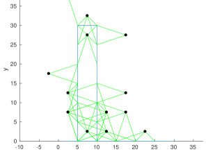
(a) Ground Truth - No Noise

(b) Random Initialization

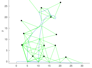
(c) Levenberg-Marquardt

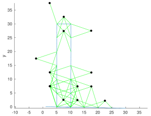
(d) SBSOS-SLAM

Figure 2: Sample estimated Landmark SLAM solution for 100 nodes of CityTrees10000 dataset [8].

(a) Ground Truth - No Noise

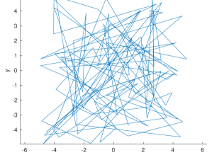
(b) Random Initialization

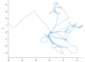
(c) Levenberg-Marquardt

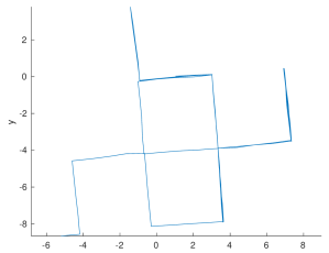
(d) SBSOS-SLAM

Figure 3: Sample estimated Pose Graph SLAM solution for 100 nodes of Manhattan3500 dataset [32].

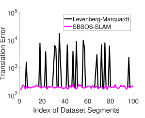
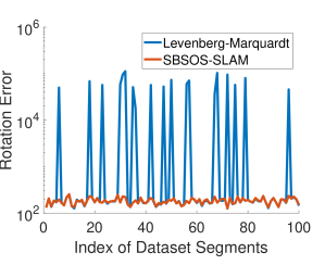
Figure 4: Translational and rotational error verses groundtruth for the CityTrees10000 dataset.

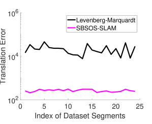
Figure 5: Translational and rotational error verses groundtruth for the Manhattan3500 dataset.

VIII-B SBSOS vs. Complex-domain SDP

We compared the SBSOS and the Complex-domain SDP (CSDP) formulations of the Rotational Averaging Problem in terms of solving time and at what level of the hierarchy the problem converges numerically. Per [9, Lemma 4] the SBSOS hierarchy convergences if the corresponding moment-based SDP, which is the dual of (26), has a rank-1 solution. Convergence of the CSDP hierarchy is checked by comparing its result against the rank-1 solution of the SBSOS formulation.

We randomly generated 500 fully connected graphs of 4,6,8,10 poses each. We then applied the SBSOS and CSDP on these graphs and evaluated their performance at the first and second steps of the hierarchy. Testing result are summarized in Table I. The SBSOS and CSDP formulations converged at the second step of the hierarchy in all evaluated examples. However, the solving time of CSDP at the second step of the hierarchy was considerably less than the solving time of SBSOS at the second step of its hierarchy. In addition, more examples converged at the first step of the CSDP hierarchy when compared to the SBSOS hierarchy.

Number of poses	SBSOS: 1st step (Mean, Std, Opt)	SBSOS: 2nd step (Mean, Std, Opt)	CSDP: 1st step (Mean, Std, Opt)	CSDP: 2nd step (Mean, Std, Opt)
4	(0.4638, 0.0577, 85.2%)	(0.4887, 0.0471, 100%)	(0.2840, 0.0367, 92.8%)	(0.2836, 0.0367, 100%)
6	(0.4003, 0.0212, 63.0%)	(2.1716, 0.1657, 100%)	(0.2600, 0.0157, 82.0%)	(0.4220, 0.0200, 100%)
8	(0.3909, 0.0216, 49.8%)	(21.1445, 1.8422, 100%)	(0.2434, 0.0155, 77.8%)	(2.9081, 0.2239, 100%)
10	(0.4310, 0.0406, 32.6%)	(148.9397, 12.2855, 100%)	(0.2954, 0.0251, 70.8%)	(23.1850, 1.1476, 100%)

TABLE I: Comparing the computation time and global convergence of the SBSOS and CSDP hierarchies on randomly generated fully connected pose graphs. Note that mean[sec] is the mean of solving time, std[sec] is the standard deviation of solving time, and opt is percentage of tests in which the problem converges.

The two formulations were also tested using the Manhattan3500 dataset with 15, 20, 25, 30 and 50 poses In each test, the initial pose of the sub-graph of the dataset was randomly chosen. The results for this test are summarized in Table II. Note that both SBSOS and CSDP formulations always converge by the second step in the hierarchy, and CSDP was considerably faster when compared to SBSOS. Note that on these subgraphs problems that were not fully connected, both SBSOS and CSDP always converged at the first step of their respective hierarchies.

Number of poses	Number of tests	SBSOS: 1st step (mean, std, opt)	SBSOS: 2nd step (mean, std, opt)	CSDP: 1st step (mean, std, opt)	CSDP: 2nd step (mean, std, opt)
15	100	(0.2553, 0.0225, 100%)	(0.9681, 2.2814, 100%)	(0.1683, 0.0165, 100%)	(0.2174, 0.1857, 100%)
20	100	(0.2225, 0.0262, 100%)	(3.6315, 12.035, 100%)	(0.1402, 0.0144, 100%)	(0.4194, 0.9496, 100%)
25	100	(0.2323, 0.0335, 100%)	(20.316, 83.996, 100%)	(0.1482, 0.0248, 100%)	(1.5447, 4.5637, 100%)
30	100	(0.2670, 0.0514, 100%)	(27.278, 101.61, 100%)	(0.2239, 0.0572, 100%)	(3.2297, 12.423, 100%)
50	23	(0.7328, 0.4335, 100%)	(527.13, 1006.4, 100%)	(0.4806, 0.2420, 100%)	(64.876, 140.94, 100%)

TABLE II: Comparing the computation time and global convergence of the SBSOS and CSDP hierarchies on randomly selected subgraphs in the Manhattan3500 dataset. Note that mean[sec] is the mean of solving time, std[sec] is the standard deviation of solving time, and opt is percentage of tests in which the problem converges.

IX Conclusion

In this paper, we proposed an algorithm called SBSOS-SLAM that formulates the planar Pose Graph and Landmark SLAM problems as polynomial optimization programs.We also described how the same problem can be implemented in the complex domain as a hierarchy of semi-definite programs. Empirical results showed that both formulations converged at the second step of the pair of hierarchies, and the implementation in complex domain was solved faster at higher hierarchical step compared to the SBSOS formulation.

References

- Cadena et al. [2016] C. Cadena, L. Carlone, H. Carrillo, Y. Latif, D. Scaramuzza, J. Neira, I. Reid, and J. J. Leonard, “Past, present, and future of simultaneous localization and mapping: Toward the robust-perception age,” IEEE Trans. on Robotics, vol. 32, no. 6, pp. 1309–1332, 2016.
- Rosen et al. [2016] D. Rosen, L. Carlone, A. Bandeira, and J. Leonard, “SE-Sync: A certifiably correct algorithm for synchronization over the Special Euclidean group,” in Proc. Int. Work. Algorithmic Foundations of Robot., 2016.
- Carlone et al. [2016] L. Carlone, G. C. Calafiore, C. Tommolillo, and F. Dellaert, “Planar pose graph optimization: Duality, optimal solutions, and verification.” IEEE Trans. on Robotics, vol. 32, no. 3, pp. 545–565, 2016.
- Rosen et al. [2015] D. M. Rosen, C. DuHadway, and J. J. Leonard, “A convex relaxation for approximate global optimization in simultaneous localization and mapping,” in Proc. IEEE Int. Conf. Robot. and Automation, Seattle, Washington, USA, May 2015, pp. 5822–5829.
- Carlone et al. [2015] L. Carlone, D. M. Rosen, G. Calafiore, J. J. Leonard, and F. Dellaert, “Lagrangian duality in 3D SLAM: Verification techniques and optimal solutions,” in Proc. IEEE/RSJ Int. Conf. Intell. Robots and Syst., Hamburg, Germany, September 2015, pp. 125–132.
- Hu et al. [2013] G. Hu, K. Khosoussi, and S. Huang, “Towards a reliable slam back-end,” in Proc. IEEE/RSJ Int. Conf. Intell. Robots and Syst., Tokyo, Japan, Nov 2013, pp. 37–43.
- Liu et al. [2012] M. Liu, S. Huang, G. Dissanayake, and H. Wang, “A convex optimization based approach for pose slam problems,” in Proc. IEEE/RSJ Int. Conf. Intell. Robots and Syst., Vilmoura, Portugal, Oct 2012, pp. 1898–1903.
- Kaess et al. [2008] M. Kaess, A. Ranganathan, and F. Dellaert, “iSAM: Incremental smoothing and mapping,” IEEE Trans. on Robotics, vol. 24, no. 6, pp. 1365–1378, 2008.
- Weisser et al. [2018] T. Weisser, J. B. Lasserre, and K.-C. Toh, “Sparse-BSOS: a bounded degree SOS hierarchy for large scale polynomial optimization with sparsity,” Mathematical Programming Computation, vol. 10, no. 1, pp. 1–32, 2018.
- Brynte et al. [2021] L. Brynte, V. Larsson, J. P. Iglesias, C. Olsson, and F. Kahl, “On the tightness of semidefinite relaxations for rotation estimation,” arXiv preprint arXiv:2101.02099, 2021.
- Lasserre et al. [2017] J. B. Lasserre, K.-C. Toh, and S. Yang, “A bounded degree SOS hierarchy for polynomial optimization,” EURO Journal on Computational Optimization, vol. 5, no. 1-2, pp. 87–117, 2017.
- Durrant-Whyte and Bailey [2006] H. Durrant-Whyte and T. Bailey, “Simultaneous localization and mapping (SLAM): Part I,” IEEE Robot. Autom. Mag., vol. 13, no. 2, pp. 99–110, 2006.
- Bailey and Durrant-Whyte [2006] T. Bailey and H. Durrant-Whyte, “Simultaneous localization and mapping (SLAM): Part II,” IEEE Robot. Autom. Mag., vol. 13, no. 3, pp. 108–117, 2006.
- Thrun et al. [2005] S. Thrun, W. Burgard, and D. Fox, Probabilistic robotics. MIT press, 2005.
- Lu and Milios [1997] F. Lu and E. Milios, “Globally consistent range scan alignment for environment mapping,” Auton. Robot., vol. 4, no. 4, pp. 333–349, 1997.
- Eustice et al. [2005] R. Eustice, M. Walter, and J. Leonard, “Sparse extended information filters: Insights into sparsification,” in Proc. IEEE/RSJ Int. Conf. Intell. Robots and Syst., Edmonton, AB, Canada, Aug 2005.
- Dellaert and Kaess [2006] F. Dellaert and M. Kaess, “Square Root SAM: Simultaneous localization and mapping via square root information smoothing,” Int. J. Robot. Res., vol. 25, no. 12, pp. 1181–1203, 2006.
- Boyd and Vandenberghe [2004] S. Boyd and L. Vandenberghe, Convex Optimization. New York, NY, USA: Cambridge University Press, 2004.
- Boumal [2015] N. Boumal, “A Riemannian low-rank method for optimization over semidefinite matrices with block-diagonal constraints,” ArXiv e-prints, Jun. 2015.
- Fan et al. [2019] T. Fan, H. Wang, M. Rubenstein, and T. Murphey, “Efficient and guaranteed planar pose graph optimization using the complex number representation,” in 2019 IEEE/RSJ International Conference on Intelligent Robots and Systems (IROS). IEEE, 2019, pp. 1904–1911.
- Fan et al. [2020] ——, “Cpl-slam: Efficient and certifiably correct planar graph-based slam using the complex number representation,” IEEE Transactions on Robotics, vol. 36, no. 6, pp. 1719–1737, 2020.
- Briales and Gonzalez-Jimenez [2017] J. Briales and J. Gonzalez-Jimenez, “Cartan-Sync: Fast and global SE(d)-synchronization,” IEEE Robot. Autom. Letters, vol. 2, 2017.
- Lasserre [2009] J. B. Lasserre, Moments, positive polynomials and their applications. World Scientific, 2009, vol. 1.
- Smail [2017] L. Smail, “Junction trees constructions in bayesian networks,” in Journal of Physics: Conference Series, vol. 893, no. 1. IOP Publishing, 2017, p. 012056.
- ApS [2015] M. ApS, The MOSEK C optimizer API manual Version 7.1 (Revision 54)., 2015. [Online]. Available: http://docs.mosek.com/7.0/capi/
- Schmidt and Spitzer [1960] P. Schmidt and F. Spitzer, “The toeplitz matrices of an arbitrary laurent polynomial,” Mathematica Scandinavica, vol. 8, no. 1, pp. 15–38, 1960.
- Gregor [1988] J. Gregor, “The multidimensional -transform and its use in solution of partial difference equations,” Kybernetika, vol. 24, no. 7, pp. 1–3, 1988.
- Horn and Johnson [2012] R. A. Horn and C. R. Johnson, Matrix analysis. Cambridge university press, 2012.
- ApS [2018] M. ApS, “Mosek modeling cookbook,” 2018.
- Wolkowicz et al. [2012] H. Wolkowicz, R. Saigal, and L. Vandenberghe, Handbook of semidefinite programming: theory, algorithms, and applications. Springer Science & Business Media, 2012, vol. 27.
- Serre [2002] D. Serre, “Matrices: Theory and applications,” 2002.
- Olson et al. [2006] E. Olson, J. Leonard, and S. Teller, “Fast iterative alignment of pose graphs with poor initial estimates,” in Proc. IEEE Int. Conf. Robot. and Automation, Orlando, Florida, May 2006, pp. 2262–2269.