Recent Improvements for the Lepton Propagator PROPOSAL

Abstract

The lepton propagator PROPOSAL is a Monte-Carlo Simulation library written in C++, propagating high energy muons and other charged particles through large distances of media. In this article, a restructuring of the code is described, which yields a performance improvement of up to $30\text{\,}\mathrm{\char 37\relax}$. For an improved accuracy of the propagation processes, more exact calculations of the leptonic and hadronic decay process and more precise parametrizations for the interaction cross sections are now available. The new modular structure allows a more flexible and custom usage, which is further facilitated with a python interface.

1 Introduction

Very large volume neutrino telescopes such as IceCube, ANTARES, GVD and the planned facilities IceCube-Gen2 and KM3net play a key role in searches for astrophysical neutrinos, the origin of cosmic rays, dark matter and exotic relic particles expected from the early universe. In all these investigations, the key process is the detection of light emitted by particles propagating through the detector and the adjacent medium. These particles, with energies from $\mathrm{GeV}$ up to several $\mathrm{PeV}$ or even $\mathrm{EeV}$, are charged leptons produced in extended air showers or neutrino interactions and possibly also heavy exotic particles.

The propagation of leptons through matter is a task, for which several codes have appeared over the years [1, 2, 3, 4, 5, 6, 7]. This article reports a major update to PROPOSAL [7], the Propagator with optimal precision and optimized speed for all leptons. The key requirements that a lepton propagator has to fulfill are a physical description that is as accurate as possible, while reducing computational errors and runtime as much as possible. To improve the accuracy of the propagation processes, precise parametrizations of the cross sections and a detailed treatment of decay processes are required.

The current version of PROPOSAL implements most recent cross section parametrizations and improves the treatment of both leptonic and hadronic decays by a more exact description of final state kinematics. The code has been restructured, which resulted in a significant increase of execution speed. The description of particles and their interaction has been changed, making heavy use of polymorphism, which facilitates the extension of PROPOSAL for the propagation of other particles; as an example, the treatment of sleptons predicted by supersymmetry is shown. Finally, a Python interface was added to allow easier usage and to enable the use of PROPOSAL in Python.

2 Updates

2.1 Updates of the code structure

The Software PROPOSAL is a further development of the former program MMC (Muon Monte Carlo) [6], which was written in Java where the version dependency of the code became a huge drawback. Therefore, PROPOSAL was developed in C++ based on MMC providing the same precision and increased performance [7]. In the first version of PROPOSAL, the code structure of MMC was reproduced. This code was now restructured to fit a more modern object-oriented C++ coding style. In particular, the data needed for the propagation routines are stored in corresponding classes, and polymorphism is used to get rid of the reliance on runtime type information.

The basic structure of the current code is shown in Fig. 1. Here the base class of PROPOSAL is the Propagator class, which holds the particle to be propagated, a geometry describing the detector volume and a list of at least one sector through which the particle is to be propagated. These parts are set once with the construction of the propagator and cannot be changed afterwards. The constructor takes a further argument, the InterpolationDef (Listing 1), which is used to determine whether to integrate or interpolate the implemented cross sections. If the interpolation is chosen, PROPOSAL saves interpolation tables in memory or on disk as determined by the InterpolationDef. These tables are sensitive to the parameters of the particle, sectors and especially the cross sections. Therefore the API prevents the user from changing the parameters of the propagator after the initialization, because the new state will not match with the generated tables. If the user needs to change the propagator, he is forced to create a new one.

In the following paragraph, the remaining three arguments of the constructor will be discussed. The first argument of the propagator is the ParticleDef, holding static data of the particle like the mass, charge, lifetime, decay modes and $e_{low}$, defining the energy below which the particle is treated as lost (defaults to the mass of the particle). The propagator creates an instance of the Particle class, a dynamic particle, out of the ParticleDef which is a composition of the static particle definition and member variables like position, energy, and momentum. The user can get a reference to the particle via a getter method to read out the information. However, the particle definition should not be changed, therefore all the members of ParticleDef are declared as const. There are several predefined particle definitions like the MuMinusDef or the TauMinusDef which are derived from the ParticleDef and obtained as singletons with MuMinusDef::Get(). To define custom particle definitions there is a ParticleDef::Builder class provided, which allows, for example, the creation of muon definitions with different masses directly from the MuMinusDef.

Listing 1: Constructor of the propagator class

⬇

1 Propagator(const ParticleDef&,

2 const std::vector<Sector::Definition>&,

3 const Geometry&,

4 const InterpolationDef&)

The core of the Propagator is defined by a list of sector definitions. In Table 1 the individual parameters are shown along with a short description. Noteworthy is the choice of a model for multiple scattering. As opposed to the previous version of PROPOSAL, two further multiple scattering models were added, which will be discussed in section 2.2. Furthermore, there is another definition object, the utility_def, which contains the definition of the individual cross section parameters for the bremsstrahlung, pair production, photonuclear interaction, and ionization. These parameters include a multiplier to manually scale the cross sections, a bool to decide whether to consider the LPM-effect (bremsstrahlung and pair production only) and an enum for the choice of the parametrization (bremsstrahlung and photonuclear interaction only).

Table 1: Description of the parameters for the sector definitions.

Parameter	Description
Medium	Medium of the sector
EnergyCutsSettings	Stores $e_{\text{cut}}$ and $v_{\text{cut}}$
Geometry	Geometry of the sector
stopping_decay	Whether to force a final decay of the particle if its energy is $\leq e_{\text{cut}}$
cont_rand	Whether to use continuous randomization
exact_time	Whether to calculation the time exactly out of the tracking integral or to use an approximation
scattering_model	Choice of the multiple scattering model, HighlandIntegral, Highland or Moliere
particle_location	Location of the particle
utility_def	Definition of cross section parameters

The main routine of the Propagator is the Propagate method shown in Listing 2. This method propagates the particle through the previously defined sectors and returns a list of secondaries expressed as DynamicData. These secondaries can be, determined by the id of this class, stochastic energy losses or particles in case of a particle decay.

Listing 2: Constructor of the propagator class

⬇

1 std::vector<DynamicData*>

2 Propagate(double MaxDistance_cm = 1e20);

Figure 1: Schematic of the main class structure.

As the programming language Python is getting more and more popular in scientific applications, a Python-interface, which can be created as a build option of PROPOSAL, is now provided. The library Boost.Python [8] is used for the interface. A typical Python code for PROPOSAL is shown in Listing 3. The comments in the listing explain some details of the different parts. In this example, a propagator is created with only one sector and $10^{6}$ muons are propagated through this sector to obtain a list of muon ranges.

Listing 3: Python code listing showing the basic instantiation of the propagator and creating data to visualize the muon ranges.

⬇

1 import pyPROPOSAL as pp

2

3 sec_def = pp.SectorDefinition()

4 sec_def.medium = pp.medium.Ice(density_correction=0.98)

5 # Init Sphere(position, outer radius, inner radius)

6 sec_def.geometry_def = pp.geometry.Sphere(pp.Vector3D(), 1e20, 0)

7

8 sec_def.scattering_model = pp.scattering.ScatteringModel.Moliere

9 sec_def.crosssection_defs.brems_def.lpm_effect = False

10 sec_def.crosssection_defs.epair_def.lpm_effect = False

11

12 sec_def.cut_settings.ecut = 500

13 sec_def.cut_settings.vcut = 0.05

14

15 interpolation_def = pp.InterpolationDef()

16 interpolation_def.path_to_tables = "~/.local/share/PROPOSAL"

17

18 prop = pp.Propagator(

19 particle_def=pp.particle.MuMinusDef.get(),

20 sector_defs=[sec_def],

21 detector=pp.geometry.Sphere(pp.Vector3D(), 1e20, 0),

22 interpolation_def=interpolation_def

23 )

24

25 mu = prop.particle

26

27 mu_length = []

28

29 for i in range(int(1e6)):

30 # Initial settings of the muon

31 mu.position = pp.Vector3D(0, 0, 0)

32 mu.direction = pp.Vector3D(0, 0, -1)

33 mu.energy = 1e6 # MeV

34 mu.propagated_distance = 0 # cm

35

36 secondaries = prop.propagate()

37

38 mu_length.append(mu.propagated_distance / 100)

The new code restructuring also has the effect of a performance gain. Previously the transition from MMC to PROPOSAL already came with a performance gain of up to $40\text{\,}\%$ [9]. This test was reproduced with the actual version of PROPOSAL and without multiple scattering to measure only the core routines. The result is shown in Fig. 2. Especially in the energy range relevant for the high energy physics, a performance gain of up to $25\text{\,}\%$ is obtained. A laptop computer with an Intel ^® Core^™ i5-4200U processor was used for these benchmarks.

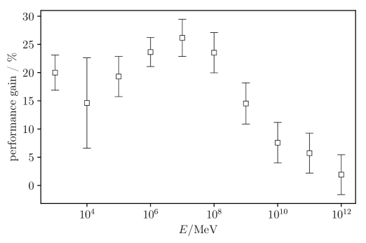
Figure 2: Runtime improvement $(t_{\text{old}}-t_{\text{new}})/t_{\text{old}}$ of the new version compared to the previous version. Multiple scattering is disabled. Per energy range $1000$ muons were propagated through ice until they lost their energy.

2.2 Physical updates

The physical improvements in the current version can be categorised in two parts; a whole restructuring of the decay process, especially for the hadronic $\tau$ decay and a broadening repertory of more accurate cross sections and multiple scattering parametrizations.

2.2.1 New Decay Implementation

The decay routines in PROPOSAL are divided into leptonic decays and hadronic decays, as already described in [7].

Leptonic Decay

For the leptonic decays, the energy distribution of the produced leptons are calculated with the differential decay width in the rest frame of the decaying lepton [10]

$$\frac{\mathrm{d}\Gamma}{\mathrm{d}x}=\frac{G_{\text{F}}^{2}M^{5}}{192\pi^{3}}(3-2x)x^{2},\quad x=\frac{E_{l}}{E_{\mathrm{max}}}$$ (1)

with the Fermi constant $G_{\text{F}}$, the mass of the decaying lepton $M$ and the limits for the energy of the produced leptons $E_{l}$ from their mass $m_{l}$ to $E_{\mathrm{max}}=(M^{2}+m_{l}^{2})/2M$.

In this parametrization of the decay width, the approximation $m_{l}^{2}/M^{2}\approx 0$ was applied, which is good for the muon decay ($m_{e}/m_{\mu}\approx 1/200$) and even better for the electronic tau decay. However, for the muonic tau decay the mass ratio ($m_{\mu}/m_{\tau}\approx 1/17$) is not small and the approximation is not valid anymore. Therefore a differential decay width without this approximation (e. g. [11]) is used

$$\frac{\mathrm{d}\Gamma}{\mathrm{d}x}=\frac{G_{\text{F}}^{2}}{12\pi^{3}}E_{\mathrm{max}}\sqrt{E_{l}^{2}-m_{l}^{2}}\left[ME_{l}(3M-4E_{l})+m_{l}^{2}(3E_{l}-2M)\right].$$ (2)

The integrated expression is, for the approximate decay width, just a polynomial ($x^{3}(1-x/2)$), while, for the more accurate decay width, it is a more complex expression

$$\int\frac{\mathrm{d}\Gamma}{\mathrm{d}x}\mathrm{d}x =\frac{G_{\text{F}}^{2}}{12\pi^{3}}\left(\frac{3}{2}m_{l}^{4}M\log(\sqrt{E_{l}^{2}-m_{l}^{2}}+E_{l})\right.$$ (3)

$$+\left.\sqrt{E_{l}^{2}-m_{l}^{2}}[(M^{2}+m_{l}^{2}-ME_{l})(E_{l}^{2}-m_{l}^{2})-1.5ME_{l}m_{l}^{2}]\right).$$ (4)

Since both integrals are not invertible, a root finding algorithm (Newton-Raphson method from [8]) is used to transform the uniformly sampled random numbers into the desired form. Therefrom the expressions are called multiple times and the higher accuracy of this parametrization goes along with a slower sampling (6 times slower) from this distribution.

The comparison between these two distributions is shown in Fig. 3.

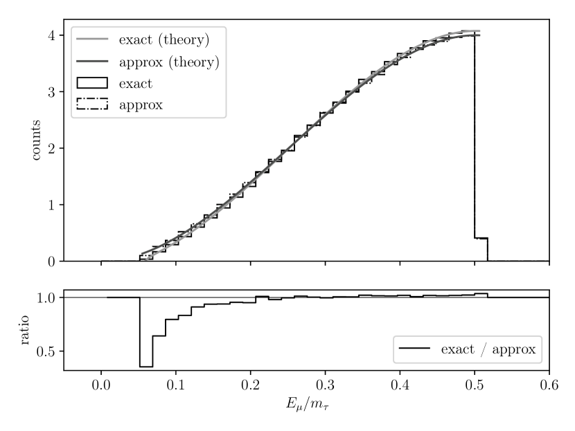
Figure 3: Normalized energy distribution of the muons in the rest frame of a muonic tau decay. Shown are the distribution with and without the approximation $m_{\mu}^{2}/m_{\tau}^{2}\approx 0$. The binned data are the results of $10^{6}$ simulated tau decays $\tau\rightarrow\mu\nu\nu$ while the solid lines represents the theoretical predictions.

Hadronic Decay

In the old version, a two body decay approximation was used for the hadronic decay [7], while leaving the matrix element constant and set to one. The hadronic secondaries produced are represented by a heavier meson or resonances, which mainly decay into the desired hadronic secondaries. The decay modes are listed in Table 2. The energy of each resonance with mass $m_{R}$ in the rest frame of the decaying lepton is $E_{\mathrm{rest}}=(M^{2}+m_{l}^{2})/2M$, which can be identified as peaks in the energy distribution of the hadronic secondaries. After boosting in the laboratory system, these peaks produce steps in the secondary energy distribution each time a new particle mass is reached, as can be seen in Fig. 4.

Table 2: Decay modes of the tau lepton used in the previous version [6].

Decay mode	Branching ratio / $\%$
$\mu$	$17.37$
$e$	$17.83$
$\pi$	$11.09$
$\rho-770$	$25.40$
$a_{1}-1260$	$18.26$
$\rho-1465$	$10.05$

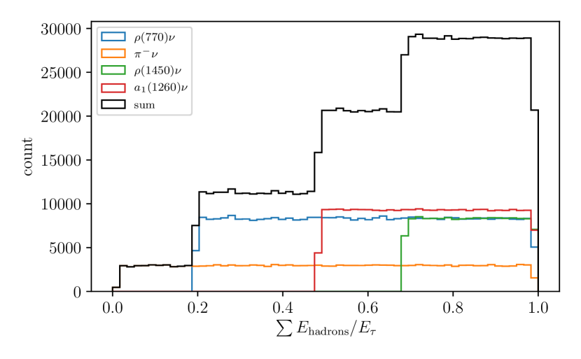
Figure 4: Energy distribution of the secondaries in the laboratory frame.

In the new version, hadronic decays are treated as $n$-body decays, increasing the phase space and smoothen the secondary distribution. For the sampling in this phase space the Raubold-Lynch algorithm [12] is used. The idea behind this algorithm is that the $n$-body phase space is recursively split up into $n$ 2-body phase spaces.

With this algorithm, more decay channels can be implemented, which can be seen in Table 3.

Table 3: Hadronic decay modes of the tau lepton with the highest branching ratios [10].

Decay mode	Branching ratio / $\%$
$\pi^{-}$	$10.82$
$K^{-}$	$0.70$
$\pi^{-}\pi^{0}$	$25.49$
$K^{-}\pi^{0}$	$0.43$
$\pi^{-}2\pi^{0}$	$9.26$
$\pi^{-}3\pi^{0}$	$1.04$
$\pi^{-}K^{0}$	$0.83$
$\pi^{-}\pi^{0}K^{0}$	$0.38$
$\pi^{-}\pi^{-}\pi^{+}$	$8.99$
$\pi^{-}\pi^{-}\pi^{+}\pi^{0}$	$2.74$
$\pi^{-}\omega$	$1.95$
$\pi^{-}\pi^{+}K^{-}$	$0.29$

With this larger phase space, the energy distribution of the decay modes with more than two particles is more smooth for the rest and laboratory system as shown in Fig. 5.

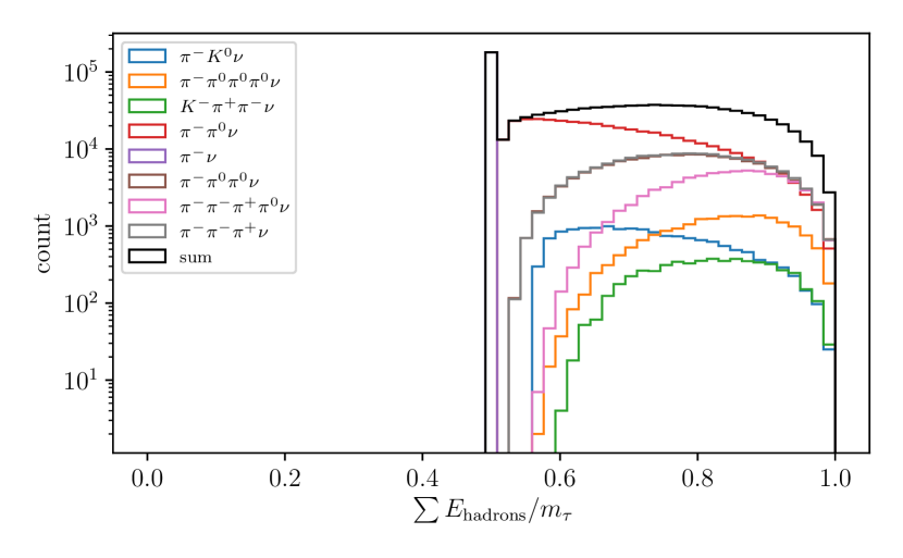
(a) rest frame

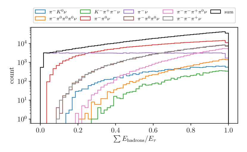
(b) laboratory frame

Figure 5: Energy distribution of the secondaries in hadronic tau decays in the rest frame (not boosted) and in the laboratory frame (boosted).

This method only improves the phase space sampling; the matrix element is still set to one. Furthermore the Raubold-Lynch algorithm does not sample the momenta uniformly distributed in the phase space. To create a uniform phase space distribution the rejection method is used, which results in a performance loss. The differences of the hadronic energy distributions between uniform and non uniform sampling are shown in Fig. 6. The performance differences can be seen in Fig. 7.

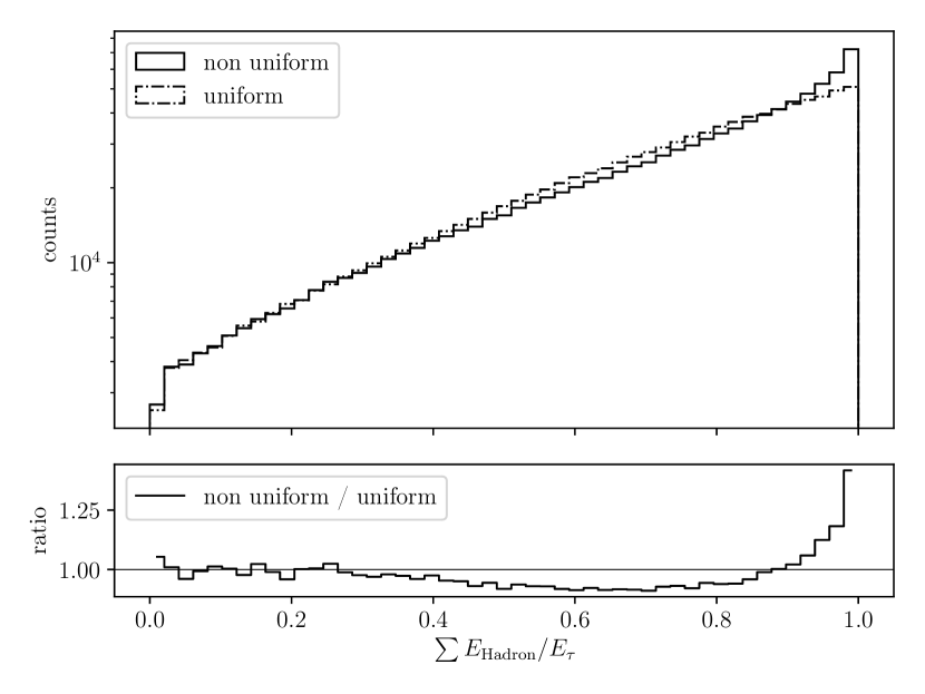
Figure 6: Comparison of the energy distributions of the secondaries for the tau decay with non uniform and uniform sampling of events in the phase phase. Shown are the results of $10^{6}$ decays with the decay channels given in Table 3.

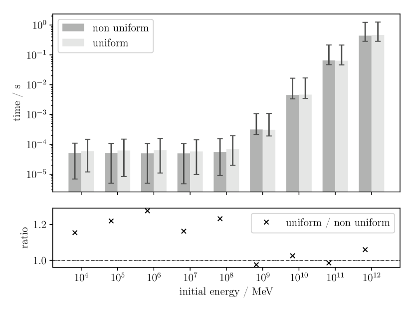
Figure 7: Comparison of run times between the non uniform and uniform phase space sampling of the tau decay with the decay channels given in Table 3. Measured are the run times of each tau propagation through ice while per energy $1000$ taus are propagated.

To illustrate the accuracy of this treatment, the leptonic decay mode with the known energy distribution is compared to the pure phase space calculation. Fig. 8 shows the pure phase space sampling of the leptonic decay with constant matrix element compared to the known energy distribution. If the sampled phase space points are now weighted with the known matrix elements for leptonic decays

$$\mathcal{M}=64G_{\text{F}}\left(p_{\tau}\cdot p_{\nu_{l}}\right)\left(p_{\nu_{\tau}}\cdot p_{l}\right)$$ (5)

the energy distribution agrees with the differential decay width, as shown in Fig. 9.

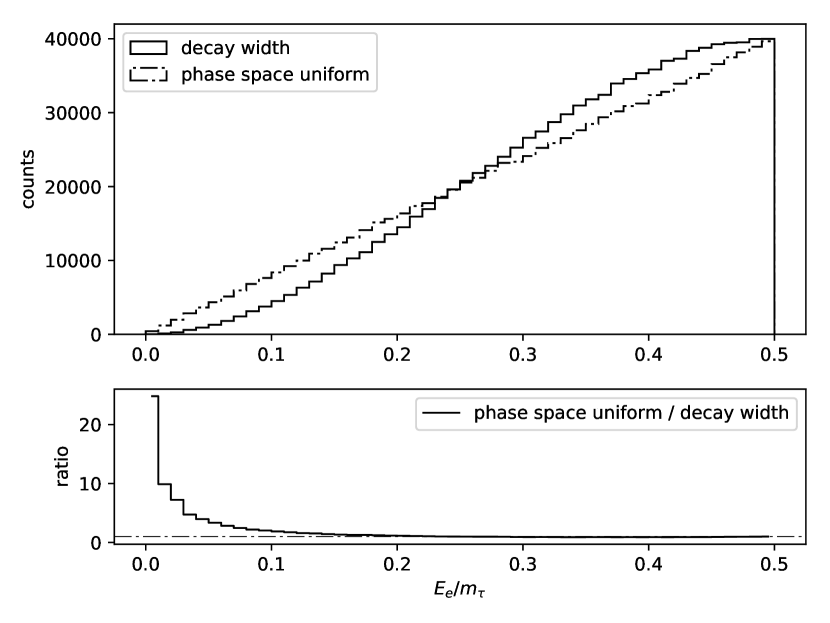
Figure 8: Comparison of the final state electron energy distribution of $\tau\rightarrow e\nu\nu$ simulated using the differential decay width and the uniform phase space sampling.

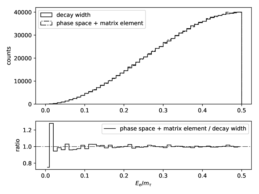
Figure 9: Comparison of the final state electron energy distribution of $\tau\rightarrow e\nu\nu$ simulated using the differential decay width and the phase space sampling with respect to the matrix element.

2.2.2 Multiple Parametrizations for systematic studies

The systematic uncertainties of the propagation mainly depend on the uncertainties of the interaction cross section. Due to the stochastic nature of the processes, a slight shift of one interaction cross section has great impacts on the probability of the occurrence of the other interactions. This results in different event signatures which influence the reconstruction and should be considered in the systematic uncertainties. Instead of simply shifting the interaction probability to study the systematic uncertainties, multiple parametrizations of the cross sections are available, which changes the probability in a more realistic way.

For bremsstrahlung and inelastic nuclear interaction, multiple parametrizations already existed in the old version. For pair production, only the [13, 14] parametrization is implemented. In the new version, a new parametrization [15], shown in A.2, without the approximation in the structure functions, describing the interaction with the target atom, is available. This approximation has an uncertainty of around $3\text{\,}\mathrm{\char 37\relax}$. To further reduce this uncertainty below $1\text{\,}\mathrm{\char 37\relax}$, radiative corrections have to be taken into account. Additionally, a new Bremsstrahlung parametrization [15], shown in A.1, also without the approximations in the structure functions and with next to leading order corrections, is now available. The effects of these new parametrizations will be illustrated in [15].

Furthermore a new parametrization for the photonuclear interaction is added. This parametrization describes the interaction of supersymmetric particles, especially charged sleptons, with nuclei under the exchange of virtual photons. The derivation of the parametrization is given in [16]. In PROPOSAL this parametrization is called PhotoRenoSarcevicSu (RSS). [16] also shows that this photonuclear interaction is the only interaction which must be treated differently from the lepton cases. The reason for adding this parametrization lies in the direct probe of the supersymmetric breaking scale by finding the supersymmetric particle stau with the IceCube detector [17]. In earlier analysis, the stau was described as a heavy muon, while using the photonuclear parametrization of Abramowicz, Levin, Levy and Maor (ALLM97) [18]. A comparison of the photonuclear parametrizations is given in Fig. 10.

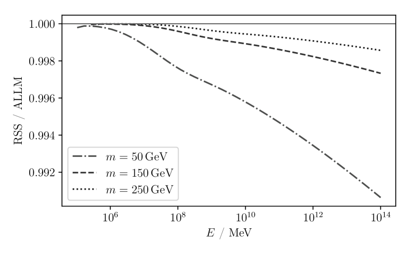
Figure 10: Shown are the energy losses $\rm{d}E/\rm{d}x$ per energy through the photonuclear interaction for heavy muons and staus with masses $m=$50\text{\,}\mathrm{G}\mathrm{e}\mathrm{V}$,$150\text{\,}\mathrm{G}\mathrm{e}\mathrm{V}$$ and $250\text{\,}\mathrm{G}\mathrm{e}\mathrm{V}$. For the muons the ALLM97 parametrization is used and for the staus the new RSS parametrization.

In addition to the new cross section parametrizations, new parametrizations for multiple scattering, which describes the deviation of the primary lepton to the shower axis, are implemented. The Highland approximation [19, 20] to the Molière scattering was implemented, with considering the decreasing energy during the propagation between two stochastic losses due to the continuous losses. To accelerate the propagation, a Highland parametrization with constant energy and no additional integration over the continuous losses is now available, although this is not a big time consuming calculation. If the precision of the position is more important than the simulation time, the original Molière algorithm [21] can be used.

To validate the implemented multiple scattering models, measured data of Akimenko et. al [22] is used. They measured the deviation of muons with a momentum of $7.3\text{\,}\mathrm{GeV}\text{\,}{\mathrm{c}}^{-1}$ traversing $1.44\text{\,}\mathrm{c}\mathrm{m}$ ($\approx 1$ radiation length) of copper. Such muons with all three implemented multiple scattering models were simulated. The comparison of the projected scattering angles $\theta$ with the data and the Monte Carlo simulation can be seen in Fig. 11. The deviations of the Monte Carlo data to the measured data is shown in Fig. 12. For this scenario the RMS of the Highland approximation is $\theta_{0}=$1.863\text{\,}\mathrm{mrad}$$. The deviation plot in Fig. 12 shows, that the Molière model is in good agreement with the data up to $4.5\cdot\theta_{0}$ whereas the Highland models are no longer acceptable when they exceed $2\cdot\theta_{0}$. In addition, Fig. 11 shows that for larger scattering angles the Molière model overestimates the measured data while both Highland models underestimate them.

Although the Molière model gives more reliable results, the performance costs are worth noting. In Fig. 13 the performance losses of all three multiple scattering models are presented compared to disabled multiple scattering. It can be seen that the propagation with the Molière scattering takes up to $250\text{\,}\%$ longer, especially for higher energies, while the performance loss for both Highland models is almost negligible. This situation is even worse when choosing a medium with more components since the Molière model is extremely sensitive to the number of components. Fig. 14 shows the same setup as Fig. 13 except for choosing ANTARES water [23] as the medium. In PROPOSAL ANTARES water is implemented with $8$ different components compared to Fréjus rock with technically one component. This causes a performance loss of up to a factor of $12$ for the propagation with Molière scattering enabled (Fig. 14). A comparison of the Highland models is given in Fig. 15. Since the integration of the original HighlandIntegral model is removed for the Highland model, the propagation with Highland scattering is slightly faster. The time measurements for this section have been performed on a laptop computer with an Intel ^® Core^™ i5-4200U processor.

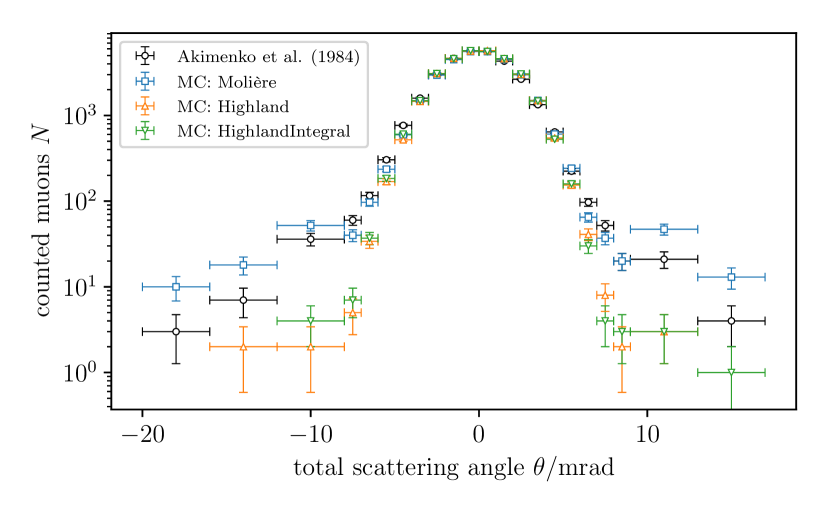
Figure 11: Measured data of $31125$ scattered muons compared with Monte Carlo simulations employing the multiple scattering model of Molière, Highland and Highland with integration.

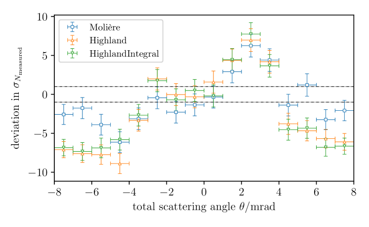
Figure 12: Deviation of the Monte Carlo data from the measurement in terms of the Poisson error of the measured data $\sigma_{N_{\text{measured}}}$.

Figure 13: Performance loss of the implemented multiple scattering models compared to disabled multiple scattering. At each energy $10^{5}$ muons are propagated $100\text{\,}\mathrm{m}$ through Fréjus rock.

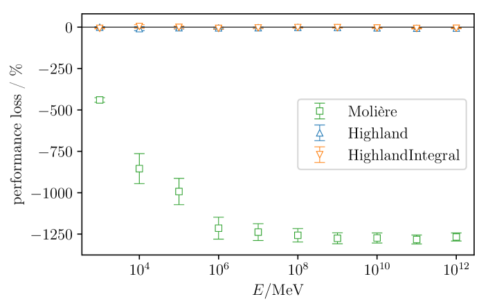
Figure 14: Performance loss of the implemented multiple scattering models compared to disabled multiple scattering. At each energy $10^{5}$ muons are propagated $100\text{\,}\mathrm{m}$ through ANTARES water [23].

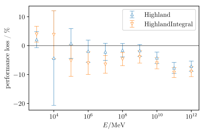
Figure 15: Performance loss of the implemented Highland and HighlandIntegral model compared to disabled multiple scattering. At each energy $10^{5}$ muons are propagated $100\text{\,}\mathrm{m}$ through Fréjus rock.

3 Conclusion

A new version of the lepton propagator PROPOSAL is presented. Compared to the previous version, computational as well as physical improvements are achieved. This new version of PROPOSAL is used in the simulation chain of the IceCube detector.

The description of particles was changed following a polymorphism paradigm. This allows one to add new particles and change the properties of already implemented particles before initialization, which is useful to investigate physics beyond the standard model and for systematic studies. The stau was added as an example of this new possibility.

In addition more recent cross sections for the energy loss processes of muons were added, and the description of hadronic tau decays was improved by dropping the two-particle decay approximation used in the previous version. This leads to more realistic secondary particle spectra.

The polymorphism and other improvements resulted in a performance increase of about $30\text{\,}\%$ compared to the previous version. This already includes the slight loss of speed due to the more exact treatment of tau decays etc.

Appendix A Improved cross section parametrizations

The cross section parametrizations reported here will be discussed in detail in a separate publication [15].

In this appendix, following symbols are used:

$B$	radiation logarithm ($\approx 183$) [24, 25]
$B^{\prime}$	inelastic radiation logarithm ($\approx 1429$) [14]
$D_{n}=1.54A^{0.27}$	nuclear formfactor parametrization [24]
$\mu$	mass of the incoming particle

A.1 Bremsstrahlung

This parametrization takes into account: elastic atomic and nuclear formfactors, inelastic nuclear formfactors, bremsstrahlung on atomic electrons ($\mu$-diagrams only), and radiative corrections.

$$\begin{split}\frac{d\sigma}{dv}&=4Z^{2}\alpha\left(r_{e}\frac{m_{e}}{\mu}\right)^{2}\frac{1}{v}\left\{\left[(2-2v+v^{2})\Phi_{1}(\delta)-\frac{2}{3}(1-v)\Phi_{2}(\delta)\right]\right.\\ &+\left.\frac{1}{Z}s_{\text{atomic}}(v,\delta)+\frac{\alpha}{4}\Phi_{1}(\delta)s_{\text{rad}}(v)\right\},\end{split}$$ (6)

where

$$\Phi_{1}(\delta) =\ln\frac{\frac{\mu}{m_{e}}BZ^{-1/3}}{1+BZ^{-1/3}\sqrt{e}\delta/m_{e}}-\Delta_{1}\left(1-\frac{1}{Z}\right),$$ (7)

$$\Phi_{2}(\delta) =\ln\frac{\frac{\mu}{m_{e}}BZ^{-1/3}e^{-1/6}}{1+BZ^{-1/3}e^{1/3}\delta/m_{e}}-\Delta_{2}\left(1-\frac{1}{Z}\right),$$ (8)

$$\Delta_{1} =\ln\frac{\mu}{q_{c}}+\frac{\rho}{2}\ln\frac{\rho+1}{\rho-1},$$ (9)

$$\Delta_{2} =\ln\frac{\mu}{q_{c}}+\frac{3\rho-\rho^{3}}{4}\ln\frac{\rho+1}{\rho-1}+\frac{2\mu^{2}}{q_{c}^{2}},$$ (10)

$$\rho =\sqrt{1+\frac{4\mu^{2}}{q_{c}^{2}}},q_{c}=m_{\mu}e/D_{n},$$ (11)

$$s_{\text{atomic}}(\delta) =\left[\frac{4}{3}(1-v)+v^{2}\right]\left[\ln\frac{\mu/\delta}{\mu\delta/m_{e}^{2}+\sqrt{e}}-\ln\left(1+\frac{m_{e}}{\delta B^{\prime}Z^{-2/3}\sqrt{e}}\right)\right],$$ (12)

$$s_{\text{rad}}(v) =\begin{cases}\sum_{n=0}^{2}a_{n}v^{n}&v<0.02,\\ \sum_{n=0}^{3}b_{n}v^{n}&0.02\leq v<0.1,\\ \sum_{n=0}^{2}c_{n}v^{n}+c_{3}v\ln v+c_{4}\ln(1-v)+c_{5}\ln^{2}(1-v)&0.1\leq v<0.9,\\ \sum_{n=0}^{2}d_{n}v^{n}+d_{3}v\ln v+d_{4}\ln(1-v)+d_{5}\ln^{2}(1-v)&v\geq 0.9,\end{cases}$$ (13)

where the values of the fit parameters $a_{n},b_{n},c_{n},d_{n}$ are given in table 4.

$n$	0	1	2	3	4	5
$a_{n}$	$-$0.00349	148.84	$-$987.531
$b_{n}$	0.1642	132.573	$-$585.361	1407.77
$c_{n}$	$-$2.8922	$-$19.0156	57.698	$-$63.418	14.1166	1.84206
$d_{n}$	2134.19	581.823	$-$2708.85	4767.05	1.52918	0.361933

Table 4: Parameters of the parametrization for the radiative corrections to the bremsstrahlung cross section.

A.2 Pair production

This parametrization of the pair production cross section takes into account: elastic atomic and nuclear formfactors, and pair production on atomic electrons.

$$\frac{d^{2}\sigma}{dv\,d\rho}=\frac{2}{3\pi}Z(Z+\zeta)\frac{1-v}{v}\left[\Phi_{e}+\frac{m_{e}^{2}}{m_{\mu}^{2}}\Phi_{\mu}\right],$$ (14)

where

$$\Phi_{e} =C_{1}^{e}L_{1}^{e}+C_{2}^{e}L_{e}^{2},$$ (15)

$$C_{1}^{e} =C_{e}-C_{2}^{e},$$ (16)

$$C_{2}^{e} =[(1-\rho^{2})(1+\beta)+\xi(3-\rho^{2})]\ln\left(1+\frac{1}{\xi}\right)+2\frac{1-\beta-\rho^{2}}{1+\xi}-(3-\rho^{2}),$$ (17)

$$L_{1}^{e} =\ln\frac{BZ^{-1/3}\sqrt{1+\xi}}{X_{e}+\frac{2m_{e}\sqrt{e}BZ^{-1/3}(1+\xi}{Ev(1-\rho^{2}}}-\frac{\Delta_{e}}{C_{e}}-\frac{1}{2}\ln\left[X_{e}+\left(\frac{m_{e}}{m_{\mu}}D_{n}\right)^{2}(1+\xi)\right]$$ (18)

$$L_{2}^{e} =\ln\frac{BZ^{-1/3}e^{-1/6}\sqrt{1+\xi}}{X_{e}+\frac{2m_{e}e^{1/3}BZ^{-1/3}(1+\xi}{Ev(1-\rho^{2})}}-\frac{\Delta_{e}}{C_{e}}-\frac{1}{2}\ln\left[X_{e}+\left(\frac{m_{e}}{m_{\mu}}D_{n}\right)^{2}e^{1/3}(1+\xi)\right]$$ (19)

$$X_{e} =\exp\left(-\frac{\Delta_{e}}{C_{e}}\right),$$ (20)

$$C_{e} =[(2+\rho^{2})(1+\beta)+\xi(3+\rho^{2})]\ln\left(1+\frac{1}{\xi}\right)+\frac{1-\rho^{2}-\beta}{1+\xi}-(3+\rho^{2}),$$ (21)

$$\Delta_{e} =[(2+\rho^{2})(1+\beta)+\xi(3+\rho^{2})]\operatorname{Li}_{2}\frac{1}{1+\xi}-(2+\rho^{2})\xi\ln\left(1+\frac{1}{\xi}\right)-\frac{\xi+\rho^{2}+\beta}{1+\xi},$$ (22)

where $L_{1,2}^{e}$ can be equivalently expressed in the case of large $X_{e}$ as

$$L_{1}^{e} =\ln\frac{BZ^{-1/3}\sqrt{1+\xi}}{1+\frac{2m_{e}\sqrt{e}BZ^{-1/3}(1+\xi)}{Ev(1-\rho^{2})}X_{e}^{-1}}-\frac{1}{2}\frac{\Delta_{e}}{C_{e}}-\frac{1}{2}\ln\left[1+\left(\frac{m_{e}}{m_{\mu}}D_{n}\right)^{2}(1+\xi)X_{e}^{-1}\right],$$ (23)

$$L_{2}^{e} =\ln\frac{BZ^{-1/3}e^{-1/6}\sqrt{1+\xi}}{1+\frac{2m_{e}e^{1/3}BZ^{-1/3}(1+\xi)}{Ev(1-\rho^{2})}X_{e}^{-1}}-\frac{1}{2}\frac{\Delta_{e}}{C_{e}}-\frac{1}{2}\ln\left[1+\left(\frac{m_{e}}{m_{\mu}}D_{n}\right)^{2}e^{1/3}(1+\xi)X_{e}^{-1}\right],$$ (24)

and

$$\Phi_{\mu} =C_{1}^{\mu}L_{1}^{\mu}+C_{2}^{\mu}L_{2}^{\mu},$$ (25)

$$L_{1}^{\mu} =\ln\frac{B\frac{\mu}{m_{e}}Z^{-1/3}/D_{n}}{X_{\mu}+\frac{2m_{e}\sqrt{e}BZ^{-1/3}(1+\xi)}{Ev(1-\rho^{2})}}-\frac{\Delta_{\mu}}{C_{\mu}},$$ (26)

$$L_{2}^{\mu} =\ln\frac{B\frac{\mu}{m_{e}}Z^{-1/3}/D_{n}}{X_{\mu}+\frac{2m_{e}e^{1/3}BZ^{-1/3}(1+\xi)}{Ev(1-\rho^{2})}}-\frac{\Delta_{\mu}}{C_{\mu}},$$ (27)

$$C_{1}^{\mu} =C_{\mu}-C_{2}^{\mu},$$ (28)

$$C_{2}^{\mu} =[(1-\beta)(1-\rho^{2})-\xi(1+\rho^{2})]\frac{\ln(1+\xi)}{\xi}-2\frac{1-\beta-\rho^{2}}{1+\xi}+1-\beta-(1+\beta)\rho^{2},$$ (29)

$$C_{\mu} =\left[(1+\rho^{2})\left(1+\frac{3}{2}\beta\right)-\frac{1}{\xi}(1+2\beta)(1-\rho^{2})\right]\ln(1+\xi)$$ (30)

$$+\frac{\xi(1-\rho^{2}-\beta)}{1+\xi}+(1+2\beta)(1-\rho^{2}),$$ (31)

$$X_{\mu} =\exp\left(-\frac{\Delta_{\mu}}{C_{\mu}}\right),$$ (32)

$$\begin{split}\Delta_{\mu}&=\left[(1+\rho^{2})\left(1+\frac{3}{2}\beta\right)-\frac{1}{\xi}(1+2\beta)(1-\rho^{2})\right]\operatorname{Li}_{2}\left(\frac{\xi}{1+\xi}\right)\\ &+\left(1+\frac{3}{2}\beta\right)\frac{1-\rho^{2}}{\xi}\ln(1+\xi)+\left[1-\rho^{2}-\frac{\beta}{2}(1+\rho^{2})+\frac{1-\rho^{2}}{2\xi}\beta\right]\frac{\xi}{1+\xi},\end{split}$$ (33)

where $L_{1,2}^{\mu}$ can be expressed for large $X_{\mu}$ equivalently as

$$L_{1}^{\mu} =\ln\frac{B\frac{\mu}{m_{e}}Z^{-1/3}/D_{n}}{1+\frac{2m_{e}\sqrt{e}BZ^{-1/3}(1+\xi)}{Ev(1-\rho^{2})}X_{\mu}^{-1}},$$ (34)

$$L_{2}^{\mu} =\ln\frac{B\frac{\mu}{m_{e}}Z^{-1/3}/D_{n}}{1+\frac{2m_{e}e^{1/3}BZ^{-1/3}(1+\xi)}{Ev(1-\rho^{2})}X_{\mu}^{-1}},$$ (35)

with the abbreviations

$$\beta =\frac{v^{2}}{2(1-v)},$$ (36)

$$\xi =\left(\frac{\mu v}{m_{e}}\right)^{2}\frac{1-\rho^{2}}{1-v},$$ (37)

$$\zeta =\frac{0.073\ln\frac{E/\mu}{1+\gamma_{1}Z^{2/3}E/\mu}-0.26}{0.058\ln\frac{E/\mu}{1+\gamma_{2}Z^{1/3}E/\mu}-0.14},$$ (38)

$$\gamma_{1} =$1.95\text{\times}{10}^{-5}$,\quad\gamma_{2}=$5.3\text{\times}{10}^{-5}$\text{ for }Z\neq 1,$$ (39)

$$\gamma_{1} =$4.4\text{\times}{10}^{-5}$,\quad\gamma_{2}=$4.8\text{\times}{10}^{-5}$\text{ for }Z=1.$$ (40)

The dilogarithm $\operatorname{Li}_{2}(x)$ is defined as

$$\operatorname{Li}_{2}(x)=-\operatorname{Re}\int_{0}^{x}\frac{\ln(1-t)}{t}dt.$$ (41)

References

- [1] V. A. Kudryavtsev, Muon simulation codes MUSIC and MUSUN for underground physics, Comp. Phys. Commun. 180 (2008) 339–346.
- [2] I. A. Sokalski, E. V. Bugaev, S. I. Klimushin, MUM: Flexible precise Monte Carlo algorithm for muon propagation through thick layers of matter, Phys. Rev. D 64 (2001) 074015.
- [3] S. Agostinelli, et al., Geant4—a simulation toolkit, Nucl. Instr. Meth. Phys. Res. A 506 (2003) 250–303.
- [4] J. Allison, et al., Geant4 developments and applications, IEEE Trans. Nucl. Sci. 53 (2006) 270–278.
- [5] J. Allison, et al., Recent developments in Geant4, Nucl. Instr. Meth. Phys. Res. A 835 (2016) 186–225.
- [6] D. Chirkin, W. Rhode, arXiv:hep-ph/0407075 (2004).
- [7] J.-H. Koehne, K. Frantzen, M. Schmitz, T. Fuchs, W. Rhode, D. Chirkin, J. B. Tjus, PROPOSAL: A tool for propagation of charged leptons, Comput. Phys. Commun. 184 (2013) 2070–2090.
- [8] A. Polukhin, Boost C++ Application Development Cookbook, Packt Publishing, Birmingham, UK, 2013.
- [9] J.-H. Köhne, Der Leptonpropagator PROPOSAL, Ph.D. thesis, TU Dortmund (2013).
- [10] M. Tanabashi, et al., Review of particle physics, Phys. Rev. D 98 (2018) 030001. doi:10.1103/PhysRevD.98.030001.
- [11] A. Lahiri, P. B. Pal, A First Book of Quantum Field Theory, 2nd Edition, Narosa Publishing House, 2004.
- [12] E. Byckling, K. Kajantie, Particle Kinematics, John Wiley and Sons, 1973.
- [13] R. P. Kokoulin, A. A. Petrukhin, Influence of the nuclear formfactor on the cross section of electron pair production by high-energy muons, in: Proc. 12th Int. Conf. on Cosmic Rays, Hobart 1971, Vol. 6, 1971, pp. 2436–2444.
- [14] S. R. Kelner, Pair production in collisions between muons and atomic electrons, Phys. At. Nucl. 61 (1998) 448–456.
- [15] A. Sandrock, et al., in Preparation.
- [16] M. H. Reno, I. Sarcevic, S. Su, Propagation of supersymmetric charged sleptons at high energies, Astropart. Phys. 24 (2005) 107–115. doi:10.1016/j.astropartphys.2005.06.002.
- [17] I. Albuquerque, G. Burdman, Z. Chacko, Neutrino telescopes as a direct probe of supersymmetry breaking, Phys. Rev. Lett. 92 (2004) 221802. doi:10.1103/PhysRevLett.92.221802.
- [18] H. Abramowicz, A. Levy, The ALLM parametrization of : an update, arXiv:hep-ph/9712415 (1997).
- [19] V. Highland, Some practical remarks on multiple scattering, Nucl Instr. Meth. 129 (2) (1975) 497–499. doi:10.1016/0029-554X(75)90743-0.
- [20] G. Lynch, O. Dahl, Approximations to multiple Coulomb scattering, Nucl. Instr. Meth. Phys. Res. B 58 (1) (1991) 6–10. doi:10.1016/0168-583X(91)95671-Y.
- [21] G. Molière, Theorie der Streuung schneller geladener Teilchen II – Mehrfach- und Vielfachstreuung, Zeitschrift für Naturforschung A 3 (2) (1948) 78–97.
- [22] S. Akimenko, V. Belousov, A. Blik, G. Britvich, V. Kolosov, V. Kutin, V. Lebedev, V. Peleshko, Y. Rastzvetalov, A. Soloviev, Multiple Coulomb scattering of 7.3 and 11.7 muons on a Cu target, Nucl. Instr. Meth. Phys. Res. A 243 (2) (1986) 518 – 522. doi:https://doi.org/10.1016/0168-9002(86)90990-3.
- [23] M. Ageron, et al., ANTARES: the first undersea neutrino telescope, Nucl. Instr. Meth. Phys. Res. A 656 (2011) 11–38.
- [24] S. R. Kelner, R. P. Kokoulin, A. A. Petrukhin, About cross section for high-energy muon bremsstrahlung, Preprint MEPhI 024-95, Moscow (1995).
- [25] S. R. Kelner, R. P. Kokoulin, A. A. Petrukhin, Radiation logarithm in the Hartree-Fock model, Phys. At. Nucl. 62 (1999) 1894–1898.