Evolutionary hypergame dynamics

Abstract

A common assumption employed in most previous works on evolutionary game dynamics is that every individual player has full knowledge about and full access to the complete set of available strategies. In realistic social, economical, and political systems, diversity in the knowledge, experience, and background among the individuals can be expected. Games in which the players do not have an identical strategy set are hypergames. Studies of hypergame dynamics have been scarce, especially those on networks. We investigate evolutionary hypergame dynamics on regular lattices using a prototypical model of three available strategies, in which the strategy set of each player contains two of the three strategies. Our computations reveal that more complex dynamical phases emerge from the system than those from the traditional evolutionary game dynamics with full knowledge of the complete set of available strategies, which include single-strategy absorption phases, a cyclic competition (“rock-paper-scissors”) type of phase, and an uncertain phase in which the dominant strategy adopted by the population is unpredictable. Exploiting the pair interaction and mean field approximations, we obtain a qualitative understanding of the emergence of the single strategy and uncertain phases. We find the striking phenomenon of strategy revival associated with the cyclic competition phase and provide a qualitative explanation.Our work demonstrates that the diversity in the individuals’ strategy set can play an important role in the evolution of strategy distribution in the system. From the point of view of control, the emergence of the complex phases offers the possibility for harnessing evolutionary game dynamics through small changes in individuals’ probability of strategy adoption.

I Introduction

Evolutionary games are a powerful mathematical and computational paradigm to gain qualitative and quantitative insights into a variety of phenomena in diverse disciplines such as biology, ecology, economics, social and political sciences Szabó and Borsos (2016); Smith (1982); Von Neumann and Morgenstern (2007); Colman (2013). A key success of evolutionary game theory is the discovery of the general principles that govern the emergence and evolution of cooperation, a phenomenon that seems to contradict the principle of natural selection, which provides a convincing explanation of its ubiquity in both animal world and human society Smith and Price (1973); Hamilton and Axelrod (1981); Dugatkin (1997); J. L. Sachs et al. (2004); Nowak (2006); Vukov et al. (2006); Szolnoki and Szabó (2007). In particular, in most previous works on evolutionary game dynamics, an assumption is that each and every player participating in the game has full knowledge about and access to the complete set of possible strategies Nowak and May (1992); Nowak et al. (1994); Ohtsuki et al. (2006); Taylor et al. (2007); Débarre et al. (2014); Allen et al. (2017). A typically studied game setting is the following: a number of agents interact with one another via some kind of network topology (e.g., regular or complex), and each agent can take on one strategy from a pre-defined strategy set determined according to the typical individual behaviors observed from real world systems, leading to classic games such as the Prisoner’s dilemma games (PDGs) Hamilton and Axelrod (1981), the snowdrift games (SGs) Sugden (1986), and the public goods games (PGGs) Hardin (1968). Such a game system typically contains two strategies: cooperation and defection, where the latter is a selfish action that usually generates immediate higher payoff Smith (1982). A remarkable achievement of evolutionary game theory is that it resolves this paradox in a counterintuitive but completely reasonable way. In fact, previous works have uncovered a variety of cooperation-facilitating mechanisms such as reputation and punishment Fehr and Gächter (2002), random diffusion Sicardi et al. (2009), memory effect Wang et al. (2006), network reciprocity Nowak and May (1992); Hauert and Doebeli (2004), random noise Szabó et al. (2005); Vukov et al. (2006, 2008), success-driven migration Helbing and Yu (2009), asymmetric cost Du et al. (2009), teaching ability Szolnoki and Szabó (2007), and social or financial diversity Santos et al. (2008); Chen et al. (2009); Chen and Lai (2012). In addition to game dynamics with two strategies (i.e., cooperation and defection), there are also games with three or more strategies, such as the “rock-paper-scissors” type of games where any strategy has a cyclic advantage over another May and Leonard (1975); Frean and Abraham (2001); Kerr et al. (2002); Szabó and Hauert (2002); Semmann et al. (2003); Reichenbach et al. (2007); Szabó and Fath (2007); Reichenbach et al. (2008); Berr et al. (2009); Wang et al. (2010); Shi et al. (2010); Yang et al. (2010); Ni et al. (2010a, b); Wang et al. (2011); Jiang et al. (2012); Park et al. (2013) and extensions Szabó and Sznaider (2004); Peltomäki and Alava (2008); Szabó et al. (2007); Szabó and Szolnoki (2008); Avelino et al. (2012); Vukov et al. (2013); Kang et al. (2013); Zheng et al. (2014); Park et al. (2017). Studies of such game dynamics have led to great insights into species coexistence and biodiversity in complex ecosystems. Theoretically, methodologies from statistical physics have been used to understand complex spatiotemporal game dynamics Szabó and Tőke (1998); Szabó and Hauert (2002); Hauert and Szabó (2005); Szabó et al. (2005); Vukov et al. (2008); Szabó and Borsos (2016).

In spite of its widespread use in previous works on evolutionary game dynamics, the assumption that every agent (game player) in the system has the same strategy set may be idealized. In reality, due to the diversity in the knowledge background and personal experience, it is only natural to assume heterogeneity in individuals’ available strategy sets. It is also possible that an individual’s strategies are affected by his/her emotions and external factors. In addition, individuals playing a game may have quite different understandings of other’s strategies. When the game players do not possess an identical strategy set because not everyone has full knowledge about the complete set of available strategies, the underlying game is called hypergame, a term coined by Bennett in 1977 Bennett (1977). In general, hypergame takes into account the realistic situation where players’ understandings and choices of the game strategies can be different. As a result, hypergame dynamics are capable of modeling competitions and conflicts in the real world more closely, leading to better and more realistic solutions than the classic game dynamics Gharesifard and Cortés (2012); Sasaki and Kijima (2012); Kovach et al. (2015). During a hypergame, an agent has his/her own knowledge base to make judgment of the environment and determines which strategy to use. The true payoff gained by the agent is determined by his/her current strategy versus the actual strategies in the system. In fact, the player’s choice of action reflects the way he/she perceives the reality and the game outcome, which is usually not accurate. The inaccuracy in the perception can affect the evolutionary dynamics of cooperation in a fundamental way, and may lead to different phenomena than predicted by classical evolutionary game dynamics in previous works.

In this paper, we study hypergame from the perspective of network dynamics. In spite of its importance, there has been little previous study of evolutionary hypergame dynamics. Because of the system complexity induced by the uncertainties in individual agent’s understanding and choice of the game strategies, we seek to construct the simplest possible class of prototypical models that retain the essential features of hypergame dynamics to uncover the underlying generic behaviors. In particular, we consider the system setting where there are three possible strategies in the system. To every agent in the system, two of the three strategies are available. During the dynamical evolution, at any given time an agent can use either one of the two available strategies with certain probabilities. The probability of adopting a strategy is thus a key (bifurcation) parameter in our model. Our computations reveal that, as the bifurcation parameter is changed, our parsimonious model generates distinct and more complex dynamical phases than those from the classical evolutionary game models. In particular, there are deterministic single-strategy-absorption phases, a “rock-paper-scissors” type phase, and a phase of high uncertainty in which the dominant strategy adopted by the population is unpredictable. We obtain an qualitative understanding of the emergence of the multiple dynamical phases by exploiting the pair approximation and solving the mean-field master equation. A striking finding is the phenomenon of strategy revival: the population adopting a specific strategy can decrease and approach zero but it can revive and dominate at later time. While qualitatively this can be explained based on cyclic competitions among three strategies, to develop a quantitative understanding is an open issue. From the network control perspective, our finding that a slight change in the bifurcation parameter can completely overturn the relative advantage between the strategies suggests that the complex game dynamics can be harnessed through small perturbations to the parameter.

II Evolutionary hypergame model

To construct a parsimonious model of evolutionary hypergame dynamics, we begin with the generalized prisoner’s dilemma game (gPDG) with three strategies: cooperation ($C$), defection ($D$), and loneliness ($L$). If an agent adopts the $L$ strategy, he/she does not actually participate in the game but nonetheless is guaranteed to receive a low payoff. For simplicity, we use the prisoner’s dilemma game model introduced by Nowak and May Nowak and May (1993), which captures the essential feature of hypergame. The payoff matrix $M$ is given by

$$\left(\begin{array}[]{cccc}&C&D&L\\ C&1&0&0\\ D&b&0&0\\ L&\sigma&\sigma&\sigma\\ \end{array}\right)$$ (1)

Because agents have a different understanding of the competition environment, during the hypergame, each agent is able to distinguish and adopt only two of the three strategies. For each agent, the resource is constrained, so the two strategies have weights that sum up to unity. There are thus three types of agents in the model: agents having available strategies (1) $C$ and $D$, (2) $D$ and $L$, and (3) $L$ and $C$, respectively. For each of the three combinations, the probability of adopting the first strategy is $\rho$ while that adopting the second strategy is $1-\rho$. For each agent, the strategy set is thus restrictively mixed because there is a missing strategy. For the whole system, there are then three distinct such strategies. Mathematically, the three strategies can be represented by the following three vectors:

$$S^{(1)} = \left(\begin{array}[]{cc}\rho\\ 1-\rho\\ 0\\ \end{array}\right),\ \ \ S^{(2)}=\left(\begin{array}[]{cc}0\\ \rho\\ 1-\rho\\ \end{array}\right),$$ (8)

$$S^{(3)} = \left(\begin{array}[]{cc}1-\rho\\ 0\\ \rho\\ \end{array}\right),$$ (12)

where rows 1, 2, and 3 indicate the adoption probabilities of strategies $C$, $D$, and $L$, respectively.

In the simulations, agents are placed on a square lattice with periodic boundary conditions. At each time step, each agent plays gPDG with its nearest neighbors. The total payoff gained is the sum of the payoffs from playing the game with all its neighbors, which is given by

$$U_{n}=\sum\limits_{m}u_{nm}=\sum\limits_{n,m}{S_{n}}^{T}MS_{m},$$ (13)

where $U_{n}$ denotes the total payoff of agent at lattice node $n$, $u_{nm}$ is the payoff obtained by agent $n$ while playing the game with agent at lattice node $m$, $M$ is the payoff matrix in Eq. (1), $S_{n}$ and $S_{m}$ are the strategy vectors of the two agents, respectively. After obtaining the payoff, agent $n$ with strategy $S_{n}$ is replaced by agent $m$ with the probability given by the Fermi rule Chen et al. (2009):

$$P_{S_{n}\longrightarrow S_{m}}=\frac{1}{1+\exp[(U_{m}-U_{n})/\kappa]},$$ (14)

where $\kappa$ measures the stochastic uncertainties (noise) characterizing irrational choices.

In each dynamical realization, initially $N$ agents with the three types of strategies are randomly distributed in the square lattice with equal probability, i.e., $F_{1}=F_{2}=F_{3}=1/3$, where $F_{x}$ is defined in Eq. (15). The system evolves in time until an equilibrium is reached. To be concrete, we set the game parameters as $b=1.02$, $\kappa=0.1$, and $\sigma=0.25$. We check to ensure that reasonably different choices of the parameters lead to qualitatively identical behaviors from the simulations. The adoption probability $\rho$ is a key parameter in the system, which is chosen as the control or bifurcation parameter.

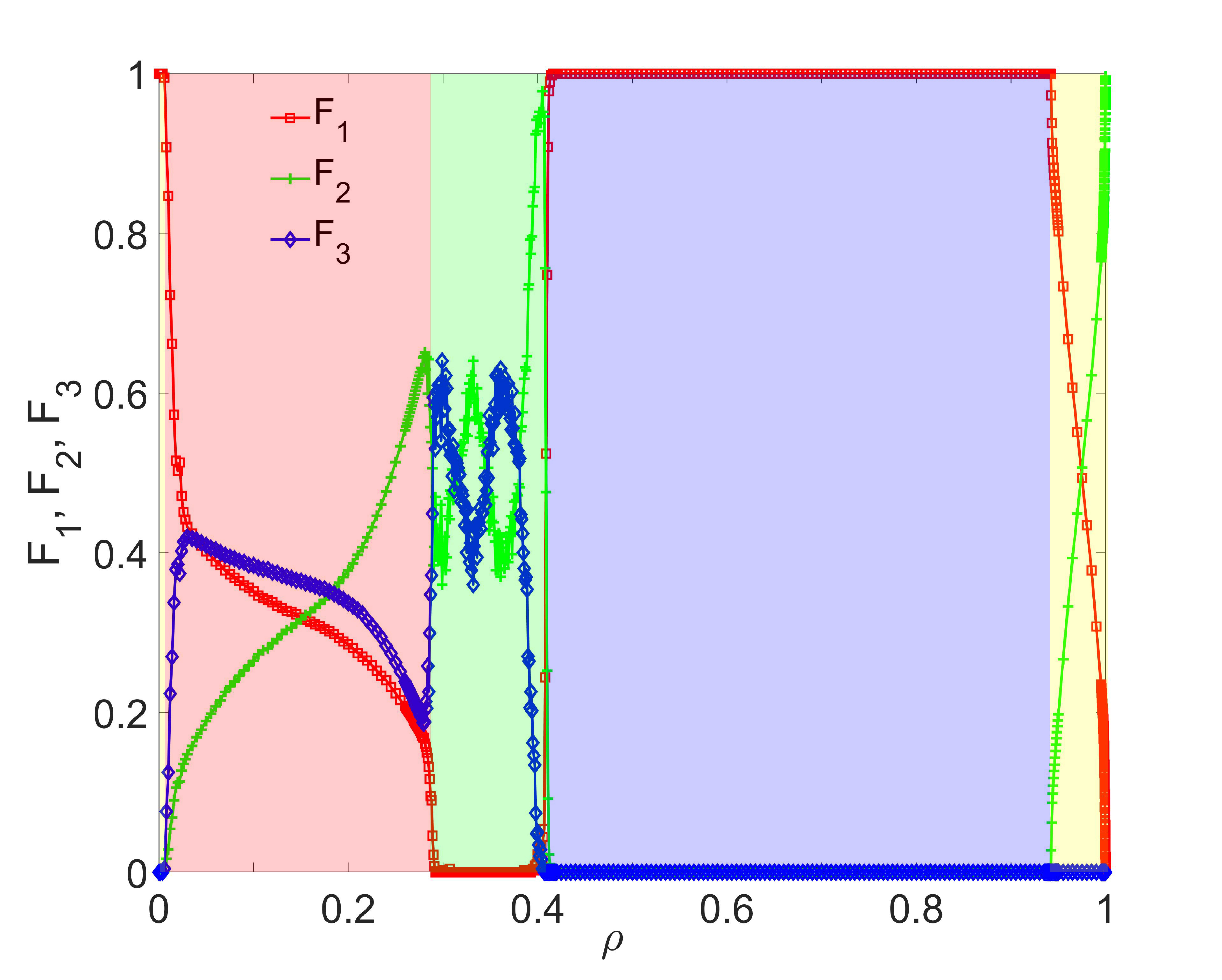
Figure 1: (Color online) Dependence of agent frequency on the bifurcation parameter. The system is a $70\times 70$ square lattice with periodic boundaries. The number of agents is $N=4900$. The red (medium gray), green (light gray) and blue (dark gray) curves show the frequencies $F_{1}$, $F_{2}$, and $F_{3}$ of the three agents versus the bifurcation parameter $\rho$, respectively. For different values of $\rho$, the system evolves into a final equilibrium state in different time $T$. In particular, for $0\leq\rho\leq 0.03$, $0.26\leq\rho\leq 0.3$, $0.935\leq\rho\leq 0.95$, and $0.995\leq\rho\leq 1$, we have $T=5\times 10^{5}$. For $0.3<\rho<0.42$, the system approaches a final state for $T<10^{4}$. For other values of $\rho$, the system needs $T=10^{4}$ time steps to approach the final state. The values of $F_{1}$, $F_{2}$, and $F_{3}$ shown are the results of averaging over 100 ensembles (random realizations) for most values of $\rho$ except for $0.3<\rho<0.42$, where 500 ensembles are used because of the relatively strong statistical fluctuations in this parameter interval. Depending on the behavior of the equilibrium strategy frequencies, the whole parameter interval can be divided into four regions: (1) $0<\rho\lesssim 0.03$ and $0.95\gtrsim\rho<1$ (region 1), (2) $0.03\lesssim\rho\lesssim 0.3$ (region 2), (3) $0.3\lesssim\rho\lesssim 0.4$ (region 3), and (4) $0.4\lesssim\rho\lesssim 0.95$ (region 4)

.

III Numerical results

III.1 The equilibrium state

The equilibrium frequency of the restrictively mixed strategy $S^{(x)}$ ($x=1,2,3$) on a square lattice of $N$ nodes is given by

$$F_{x}=\frac{\sum\limits_{n=1}^{N}I(S_{n},S^{(x)})}{N},$$ (15)

where $S_{n}$ denotes the strategy of agent at lattice node $n$ and $I(S_{n},S^{(x)})$ is an indicator function [$I(S_{n},S^{(x)})=1$ for $S_{n}=S^{(x)}$ and $I(S_{n},S^{(x)})=0$ otherwise]. We use 100 random simulation realizations to obtain the value of $F_{x}$. Figure 1 shows the frequencies $F_{1}$, $F_{2}$, and $F_{3}$ associated with the strategies $S^{(1)}$, $S^{(2)}$, and $S^{(3)}$, respectively, versus the parameter $\rho$. In different regions of $\rho$ value, the frequencies exhibit dramatically different behaviors. Specifically, for $\rho\gtrsim 0$, $S^{(1)}$ dominates the entire population, while the frequencies of $S^{(2)}$ and $S^{(3)}$ are essentially zero. As $\rho$ is increased, a sharp reduction in $F_{1}$ occurs, leading to an increase in the values of both $F_{2}$ and $F_{3}$. At this point, the system enters into a state in which strategies coexist with similar frequency values. When $\rho$ reaches the value of about $0.3$, the value of $F_{1}$ becomes effectively zero, while those of $F_{2}$ and $F_{3}$ alternate. For $\rho\approx 0.4$, $F_{2}$ peaks, indicating that $S^{(2)}$ now dominates the system. With a small increment in the value of $\rho$, $S^{(1)}$ becomes dominant, after which the system remains in the $S^{(1)}$-absorption state for a large range of the $\rho$ value until about $\rho\approx 0.94$ when the gradual increase and decrease in the values of $F_{2}$ and $F_{1}$, respectively, drive the system into an $S^{(2)}$-absorption state at $\rho=1$. We thus see that, as $\rho$ is changed, the system shows highly complex behaviors with distinct evolutionary patterns. For example, one strategy may have superior advantage over the others in some parameter region but may lose appeals completely in other regions. The phase transitions associated with most of the dramatic changes in the system dynamics are abrupt. This numerical finding indicates that hypergame dynamics can be much richer than conventional game dynamics with pure strategies.

For convenience, we use different colors to denote the four regions with qualitatively different behaviors (i.e., different phases), as shown in Fig. 1. From the model setting, we see that each of the three strategy vectors can get infinitesimally close to another for $\rho\rightarrow 0$ or $\rho\rightarrow 1$: $S^{(1)}|_{\rho\rightarrow 0}\rightarrow S^{(2)}|_{\rho\rightarrow 1}$, $S^{(2)}|_{\rho\rightarrow 0}\rightarrow S^{(3)}|_{\rho\rightarrow 1}$, and $S^{(3)}|_{\rho\rightarrow 0}\rightarrow S^{(1)}|_{\rho\rightarrow 1}$, providing an explanation for the similarities in the behaviors of $F_{1}$, $F_{2}$, and $F_{3}$ for $\rho\rightarrow 0$ and $\rho\rightarrow 1$. For this reason, the regions corresponding to $\rho\rightarrow 0$ and $\rho\rightarrow 1$ are marked with the same color.

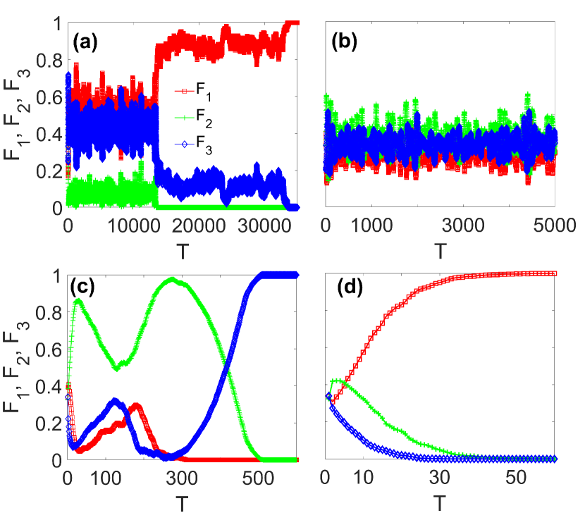
Figure 2: (Color online) Transient behaviors associated with hypergame dynamics. (a-d) Transient behaviors in the evolution of the restrictively mixed strategies for $\rho=0.001$ (in region 1), $\rho=0.2$ (in region 2), $\rho=0.31$ (in region 3) and $\rho=0.7$ (in region 4), respectively. The red (medium gray), green (light gray), and blue (dark gray) curves represent the fractions of $S^{1}$, $S^{2}$, and $S^{3}$, respectively, where $T$ is the number of evolution time steps. The results from all four panels are from a single realization of the system. The system parameters are the same as those in Fig. 1.

III.2 Transient behaviors

The transient behaviors that the system exhibits before approaching the equilibrium reveal more about the hypergame dynamics than the equilibrium itself. For example, in region 1 ($0<\rho\lesssim 0.03$ and $0.95\gtrsim\rho<1$), there are two restrictively mixed strategies: $S^{(1)}$ and $S^{(3)}$ on the left side of $\rho=0$ (or $S^{(2)}$ and $S^{(3)}$ on the right side of $\rho=1$), where the strategy with a stronger defective weight gains evolutionary advantage over the one with more cooperative weight while the third strategy disappears long before the equilibrium is reached, as shown in Fig. 2(a). This is due to that, when the value of $\rho$ is near zero or unity, the restrictively mixed strategies are similar to the pure strategies in traditional game dynamics, where the defective strategy dominate on networks with a homogeneous topology due to fluctuations and the finite size effect. In this case, the third strategy has little chance to lead to high payoff and would be eliminated quickly, so the final state is the coexistence of two restrictively mixed strategies. In region 2 ($0.03\lesssim\rho\lesssim 0.3$), the final state is the coexistence of all three restrictively mixed strategies. In this case, no strategy can be eliminated, as shown in Fig. 2(b). The rapid increase in the frequency of $S^{(2)}$ for $\rho$ close to $0.1$ indicates that a slight increment in $\rho$ can reactivate the strategy $S^{(2)}$ and a small amount of defection can lead to a substantial increase in the evolutionary fitness. As the value of $\rho$ approaches $0.3$, the strategy $S^{(2)}$ becomes relatively dominant, while the strategies $S^{(1)}$ and $S^{(3)}$ approach extinction, as shown in Fig. 2(c). As $\rho$ passes through a certain threshold value, the system enters into region 3 ($0.3\lesssim\rho\lesssim 0.4$), in which the transient behavior can be complicated but the equilibrium falls into only one of two states: the $S^{(2)}$ or the $S^{(3)}$ absorption state. This means that a single strategy always wins, either $S^{(2)}$ or $S^{(3)}$. The frequencies of $S^{(2)}$ and $S^{(3)}$ shown in Fig. 1 are ensemble averaged values of the number of agents in the $S^{(2)}$ and $S^{(3)}$ absorption states, respectively, where a single realization leads to a state with only one strategy: $S^{(2)}$ or $S^{(3)}$. Strikingly, before the equilibrium is reached, $S^{(1)}$ and $S^{(3)}$ enter into a nearly extinction state, where their frequencies are so low that random fluctuations can eliminate one of them. However, if $S^{(1)}$ becomes extinct, $S^{(3)}$ will take over the entire system. Figure 2(c) also shows the dramatic change in the frequency of $S^{(3)}$. The coexistence of the three strategies lasts longer for a larger network, so $S^{(1)}$ and $S^{(3)}$ are more resilient to random fluctuations. In region 4 ($0.4\lesssim\rho\lesssim 0.95$), $S^{(1)}$ take over after it wins the competition with $S^{(2)}$, while $S^{(3)}$ survives only in the first few time steps. The final state is one dominated by $S^{(1)}$.

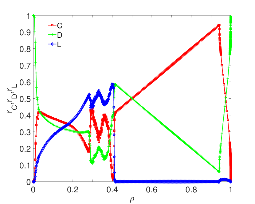
Figure 3: (Color online) Actual fractions of cooperation, defection, and loneliness. These fractions are denoted by $r_{C}$, $r_{D}$, $r_{L}$, respectively, which depend on the value of $\rho$ in a somewhat complicated manner. However, there are parameter regions in which cooperation dominates, e.g., $0.5\lesssim\rho\lesssim 0.95$. Simulation parameters are the same as those in Fig. 1.

III.3 Fraction of cooperation

The fraction of cooperation is a more intuitive characterizing quantity of the system dynamics. Figure 3 shows the actual fractions of cooperation, defection, and loneliness versus $\rho$. While the dependence of the fraction of cooperation on $\rho$ is complicated, there are parameter regions in which cooperation dominates, e.g., $0.5\lesssim\rho\lesssim 0.95$, For $\rho\approx 0.95$, the fraction of cooperation is nearly one.

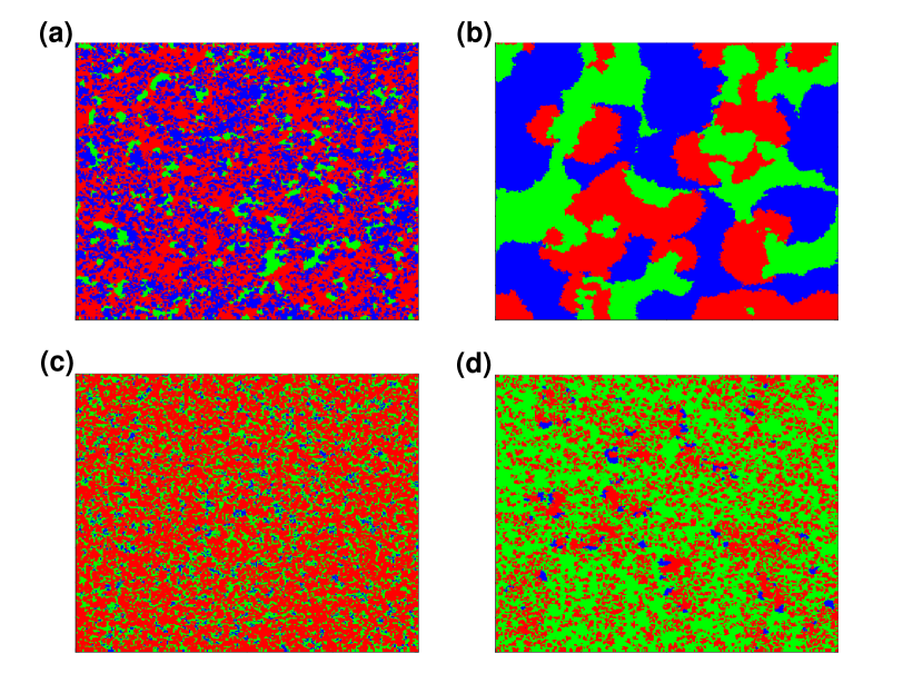
Figure 4: (Color online) Snapshots of typical lattice configuration for different $\rho$ values. (a-d) Snapshots of self-organizing patterns on the lattice associated with equilibrium coexistence of $S^{(1)}$ [red (medium gray)], $S^{(2)}$ [green (light gray)], and $S^{(3)}$ [blue (dark gray)] for $\rho=0.01,0.35,0.65$ and $0.99$, respectively. Other parameters are $b=1.02$, $\sigma=0.25$, and $K=0.1$. The lattice size is $400\times 400$.

Figure 5: (Color online) Strategy revival. (a,f,g,h,i) For $\rho=0.35$, the patterns of $S^{(1)}$ [red (medium gray)], $S^{(2)}$ [green (light gray)], $S^{(3)}$ [blue (dark gray)] on the square lattice of size $400\times 400$. (b-e) Magnification of the patterns at different time. Other parameters are the same as in Fig. 4.

Figure 6: (Color online) Persistence of strategy revival in small world networks. (a-c) The small world networks are generated by randomly rewiring $1\%$, $1.5\%$, $2\%$ of the links of the square lattice, respectively. In all cases, there is strategy revival, in spite of an increase in the time that it takes for it to occur. This time can be reduced by increasing the average degree of the network, as shown in (d) for $\langle k\rangle=8$. The network size for (a-d) is $160000$. The value of the parameter $\rho$ is 0.35 for (a-c) and 0.325 for (d). All other parameters are the same as in Fig. 5.

Figure 7: (Color online) Frequency of a dominant state. The frequency values for the system to exhibit an $S2$ or an $S3$ dominant state. All data points are the result of averaging over 500 statistical ensembles. The red (medium gray), green (light gray), and blue (dark gray) curves represent $S1$, $S2$, and $S3$, respectively. (a-d) The frequencies of $S2$ and $S3$ for a $70\times 70$, $200\times 200$, $250\times 250$, and $400\times 400$ lattice, respectively. Periodic boundary conditions are used.

III.4 Evolution pattern on lattice and strategy revival

To further understand the coexistence of strategies for values of $\rho$ in distinct dynamical regimes, we compute the patterns of the equilibrium coexistence states on the lattice, as shown in Fig. 4. In region 1, on the right side of $\rho=0$, before an equilibrium state is reached, a typical pattern is that $S^{(3)}$ forms small but relatively stable clusters with irregular boundaries distributed evenly on the lattice. In between the clusters is $S^{(1)}$, as shown in Fig. 4(a). A similar phenomenon occurs on the near left of $\rho=1$ for strategies $S^{(2)}$ and $S^{(1)}$. In region 2, $S^{(1)}$ and $S^{(3)}$ form large clusters with regular boundaries, while $S^{(2)}$ acts as the background of those clusters, as shown in Fig. 4(b). Frequent strategy transitions occur on the boundaries. For example, on the boundary between $S^{(1)}$ and $S^{(2)}$, the probability of $S^{(1)}$ transforming into $S^{(2)}$ is higher than that of the transformation in the opposite direction. On the boundary between $S^{(2)}$ and $S^{(3)}$, $S^{(3)}$ is more likely to replace $S^{(2)}$, and on the boundary between $S^{(1)}$ and $S^{(3)}$, $S^{(1)}$ is more likely to exclude $S^{(3)}$. This interaction pattern is effectively that of a cyclic (rock-paper-scissors - RPS) game. Closer to region 3, the frequencies of $S^{(1)}$ and $S^{(3)}$ in the equilibrium states decrease continuously, indicating the possible occurrence of a region in which only $S^{(2)}$ exists as $\rho$ is increased. However, this cannot occur for the reason that, in region 3, the existence of $S^{(3)}$ is robust, as shown in Fig. 4(b). In particular, in this parameter region, for a long period of time, the transient evolution patterns of the three strategies are similar to those associated with the RPS-like game in which all three strategies coexist. Surprisingly, after a long time evolution, $S^{(1)}$ or $S^{(3)}$ can suddenly disappear as their frequencies approach zero, which breaks the symmetry: if $S^{(1)}$ becomes extinct first, $S^{(3)}$ would eventually take over the entire network since $S^{(3)}$ is more likely to replace $S^{(2)}$. Likewise, if $S^{(3)}$ disappears before $S^{(1)}$, the $S^{(2)}$ absorption state will finally be realized, since there is a higher probability for $S^{(2)}$ to exclude $S^{(1)}$. The emergence of distinct equilibrium states, namely the $S^{(2)}$ or the $S^{(3)}$ absorption state, depends on which strategy [$S^{(1)}$ or $S^{(3)}$] becomes extinct first. In region 4, there is no clustering behavior, and $S^{(1)}$ takes over the entire lattice rapidly. (See Supplementary Videos Sup for a vivid presentation of the different evolution processes.)

Figure 5 shows a concrete example of the striking phenomenon of strategy revival: $S^{(3)}$ takes over the entire lattice system even when it has become almost extinct at a time (in region 3). In particular, Fig. 5(a) shows that the system can reach a state in which there is only a single $S^{(3)}$ cluster of extremely small size in contact with a small size $S^{(1)}$ cluster. Figures 5(d-f) show the evolution pattern after the state in Fig. 5(c) has been reached. We see that, the smaller $S^{(1)}$ cluster first collapses into several components and the part still in contact with $S^{(3)}$ disappears, leaving a cluster of $S^{(3)}$ surrounded by $S^{(2)}$ only, while the other $S^{(1)}$ regions are surrounded by $S^{(2)}$. The $S^{(1)}$ and $S^{(3)}$ clusters become well separated, leading to the dominance of $S^{(3)}$: $S^{(1)}$ would eventually be replaced by the surrounding $S^{(2)}$. When no $S^{(1)}$ is left, no matter how few $S^{(3)}$ holders there are, they will exclude all the $S^{(2)}$ holders and overturn the whole square lattice into the $S^{(3)}$ absorption state. Without the separation, $S^{(3)}$ would be completely excluded by $S^{(1)}$ at certain time. In this case, when there are only $S^{(1)}$ and $S^{(2)}$ left, $S^{(2)}$ will take over by excluding all $S^{(1)}$. This is the mechanism by which the $S^{(2)}$ absorption state is generated.

Figure 6 shows that the phenomenon of strategy revival can also occur in networks with a more complex structure than a regular lattice. In particular, the networks in Figs. 6(a-c) are constructed from a regular square lattice with three different percentages of link rewiring to generate long range random links - they are small world networks. There is strategy revival in all three networks, in spite of the increase in the time for the system to reach the state in which the strategy $S^{(1)}$ is extinct and eventually replaced by the strategy $S^{(3)}$. The time can be reduced by increasing the average degree of the network, as exemplified in Fig. 6(d).

To better visualize the spatiotemporal evolution of patterns, we provide four Supplementary movies Sup .

III.5 Emergence of a dominant state

Figure 7 shows the frequencies of the three restrictively mixed strategies versus the control parameter $\rho$. There exist parameter regions where one of the strategies dominates. For $0.32\lesssim\rho\lesssim 0.4$, the dominant strategy can be either $S^{(2)}$ or $S^{(3)}$. The frequencies also depend on the system size. For small systems, the frequency values for $S^{(2)}$ and $S^{(3)}$ (green and blue curves) oscillate about the value of $0.5$ as $\rho$ is varied in the interval. There are three distinct points of $\rho$ at which the two probabilities are equal. As the system size is increased, there exists only one such value of $\rho$. For example, for $\rho\in[0.32,0.36]$, the probability for $S^{(3)}$ to be dominant increases with system size. For $\rho\in[0.36,0.4]$, $S^{(2)}$ will dominate for relatively large systems.

IV Theory

Figure 8: (Color online) Boundary structure of clusters and agents in an eight-node motif. In (a), the red (dark gray), green (light gray), and blue (medium gray) nodes represent the target agent, the opponent node, and the neighbors of this pair of nodes, respectively. (b) The cluster boundary structure, where there are two types of agents. The upper part of the panel appears on the boundary of the large cluster, while others arise on the boundary of the small cluster. The boundaries of the various clusters typically contain two types of agents. The red and green nodes in (b) represent two types of agents.

Index of structure	1	2	3	4	5	6
1	S1	S1	S1	S1	S1	S1
2	S1	S1	S1	S1	S1	S2
3	S1	S1	S1	S1	S1	S3
4	S1	S1	S1	S1	S2	S1
…	…	…	…	…	…	…
729	S3	S3	S3	S3	S3	S3

Table 1: Indexing scheme for the six neighbor structures

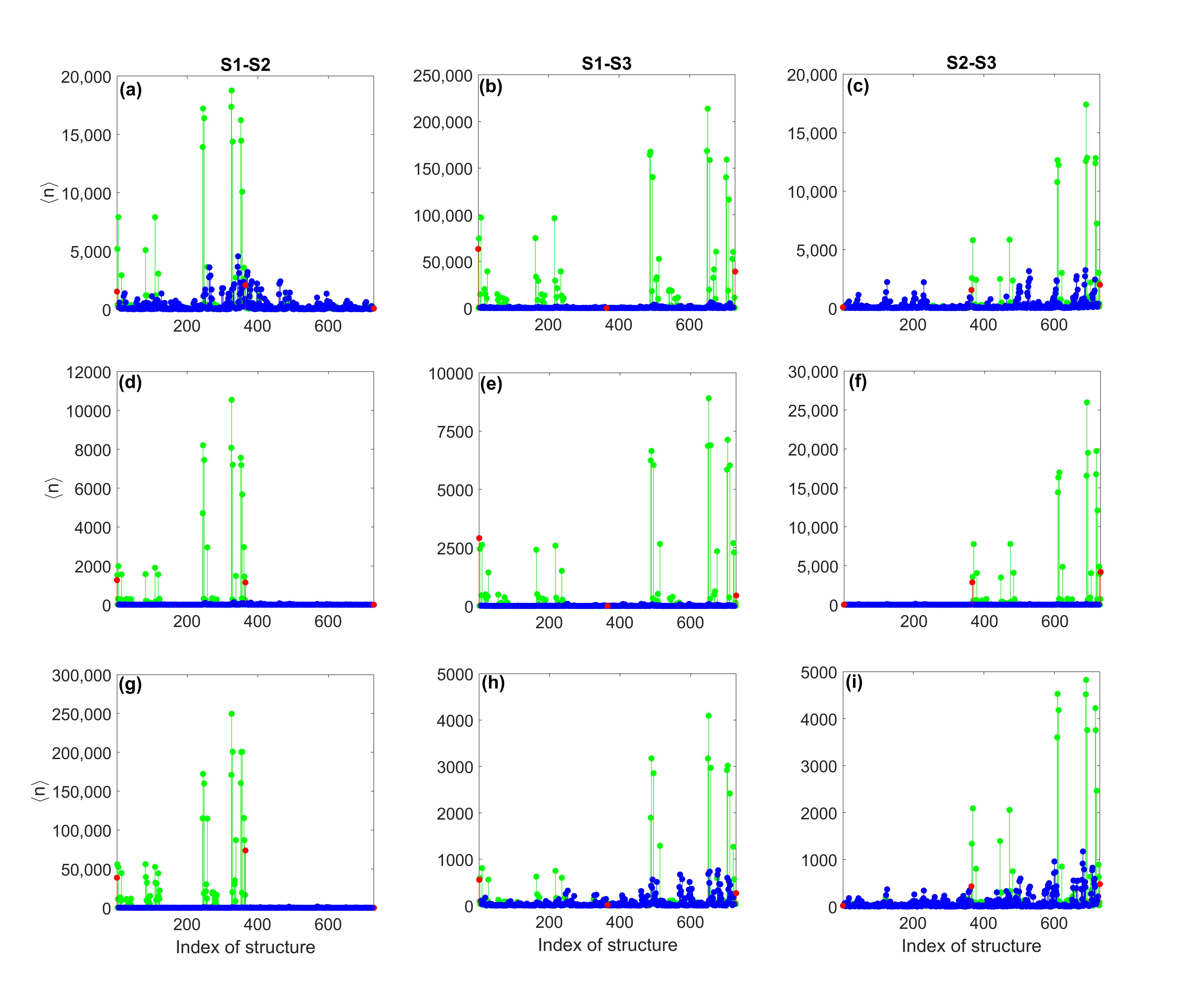
Figure 9: (Color online) Statistical distribution of distinct strategy configurations. (a-i) Counts of every neighboring structure from simulation data, where the red (medium gray), green (light gray), and blue (dark gray) dots represent the cases where there is only one type, two types, and three types of agents within the six neighbors [Fig. 8(a)], respectively. The values of the parameter $\rho$ are: $\rho=0.01$ for (a-c), $\rho=0.35$ for (d-f), and $\rho=0.99$ for (g-i). The distinct boundary structures are: target agent $S^{(1)}$ versus opponent agent $S^{(2)}$ (a,d,g), $S^{(1)}$ versus $S^{(3)}$ (b,e,h), and $S^{(2)}$ versus $S^{(3)}$ (c,f,i). For each panel, the structure index is an encoding of the six neighbors in Fig. 8(a), where are 729 such combinations. All data points are the result of taking the average between time steps 251 and 300. The lattice size is $400\times 400$.

IV.1 Modeling of interaction configurations and pair approximation on interaction motifs

Methods of theoretical analysis of the evolutionary dynamics on square include the mean-field theory Szabó et al. (2005) in combination with pair approximation Wu and Wang (2007); Perc and Marhl (2006); Hauert and Szabó (2005) and the master equation Gleeson (2013). To develop a theoretical understanding of complex dynamical behaviors as exemplified in Figs. 1-4, we take the mean field/pair approximation approach. To enumerate the possible pairwise interactions, we assume that each strategy exists in the clusters of the agents adopting that strategy (Fig. 4), so the interactions (strategy transitions) occur only at the boundaries of the clusters between different strategies. Figure 8(a) shows the typical configurations of pair interactions on a square lattice, where the two focal nodes are surrounded by six other nodes, and each of the eight nodes can adopt any of the three strategies. However, the boundaries between the clusters of different strategies typically contain two distinct strategies only, which can be empirically verified via the statistics of the strategy distribution configurations of the eight-node motif.

For two clusters with regularly shaped boundaries, there are altogether six typical configurations of strategies on the eight-node motif, as shown in Fig. 8(b). The focal node on the left and its left neighbor can be assumed to have the same strategy, as they belong to the same cluster. The upper and lower neighbors of the focal node can have the same strategy or the strategy of the other focal node on the right, which is different from that of the left focal node. Similarly, the focal node on the right and its right neighbor are in the same cluster and thus have the same strategy, while its upper and lower neighbor can choose to have either of the two strategies freely. Due to the fact that the payoff of each focal node depends only on the number of its neighbors in each type of two strategies, symmetric configurations are regarded as the same. Consequently, there are only six distinct cases, which are denoted as configurations (1-6) in Fig. 8(b). For boundaries with an irregular shape, the left (or right) neighbor of the left (or right) focal node on the motif may have a different strategy. Accordingly, there are three additional configurations, denoted as cases (7-9) in Fig. 8(b). Given two distinct strategies, $S^{(x)}$ and $S^{(y)}$, the payoffs of the two focal nodes in each of the nine configurations can be calculated. Furthermore, under the assumption that the nine configurations occur with equal probability, the average payoff of each focal node can be obtained, leading to the probability $P_{S^{(x)}\rightarrow S^{(y)}}$ of a focal node to replaced by its opponent focal node, namely, the probability for the strategy of a focal node to be excluded by that of the other focal node.

To gain insights, we study the statistical distributions of distinct strategy configurations, with results shown in Fig. 9. The coding scheme of the six-neighbor structures is shown in Table 1. We see that the green dots occur most frequently at the cluster boundaries, indicating that the boundaries are mostly between two types of agents. The most frequently occurring boundary structures are those shown Fig 8(b). From Fig. 4, we see that there are more small clusters for $\rho=0.01$ or $\rho=0.99$ than for $\rho=0.35$. The six large cluster boundary structures appear more often for $\rho=0.35$. For $\rho=0.01$, the frequencies of $S^{(1)}$ and $S^{(3)}$ are larger than that of $S^{(2)}$. There are many more boundary points between $S^{(1)}$ and $S^{(3)}$ than any other combinations of agent pairs. Based on the two types of agent boundaries and the nine kinds of cluster boundaries, we can exploit the mean field theory (below) to calculate the theoretical transfer probability for any type of agents and predict their frequencies.

The various probabilities of strategy adoptions can be calculated by resorting to the pairwise interaction approximation. For each of the nine strategy distribution configurations on the eight-node interaction motif in Fig. 8, the payoffs of the two focal nodes with strategies $S^{(x)}$ and $S^{(y)}$ are $U_{x}^{(1)}=(u_{xx}+u_{xy})+2u_{xx}$, $U_{y}^{(1)}=(u_{yy}+u_{yx})+2u_{yx}$, $U_{x}^{(2)}=(u_{xx}+u_{xy})+2u_{xx}$, $U_{y}^{(2)}=(u_{yy}+u_{yx})+u_{yx}+u_{yy}$, $U_{x}^{(3)}=(u_{xx}+u_{xy})+u_{xx}+u_{xy}$, $U_{y}^{(3)}=(u_{yy}+u_{yx})+u_{yx}+u_{yy}$, $U_{x}^{(4)}=(u_{xx}+u_{xy})+2u_{xx}$, $U_{y}^{(4)}=(u_{yy}+u_{yx})+2u_{yy}$, $U_{x}^{(5)}=(u_{xx}+u_{xy})+u_{xx}+u_{xy}$, $U_{y}^{(5)}=(u_{yy}+u_{yx})+2u_{yy}$, $U_{x}^{(6)}=(u_{xx}+u_{xy})+2u_{xy}$, $U_{y}^{(6)}=(u_{yy}+u_{yx})+2u_{yy}$, $U_{x}^{(7)}=(u_{xx}+u_{xy})+u_{xx}+u_{xy}$, $U_{y}^{(7)}=(u_{yy}+u_{yx})+2u_{yx}$, $U_{x}^{(8)}=(u_{xx}+u_{xy})+2u_{xy}$, $U_{y}^{(8)}=(u_{yy}+u_{yx})+u_{yx}+u_{yy}$, $U_{x}^{(9)}=(u_{xx}+u_{xy})+2u_{xy}$, and $U_{y}^{(9)}=(u_{yy}+u_{yx})+2u_{yx}$, where $(x,y)=1,2,3$ but $x\neq y$. The quantities $u_{xx}$, $u_{xy}$, $u_{yx}$, and $u_{yy}$ denote the payoffs of one focal node with strategies $S^{(x)}$, $S^{(x)}$, $S^{(y)}$, $S^{(y)}$ against an opponent node with strategies $S^{(x)}$, $S^{(y)}$, $S^{(x)}$, and $S^{(y)}$, respectively. The quantity $U_{x}^{(i)}$ (or $U_{y}^{(i)}$) stands for the total payoff obtained by the focal node with strategy $S^{(x)}$ (or $S^{(y)}$) in configuration $i$ in the games with its four opponents. Accordingly, the probability for a focal node with strategy $S^{(x)}$ to be replaced by its opponent focal node with strategy $S^{(y)}$ can be calculated as

$$P_{S^{(x)}\rightarrow S^{(y)}}=\frac{1}{1+\exp[(\langle{U_{y}}\rangle-\langle{U_{x}}\rangle)/K]},$$ (16)

where $\langle{U_{x}}\rangle=1/9\cdot\sum_{i=1}^{9}U_{x}^{(i)}$ and $\langle{U_{y}}\rangle=1/9\cdot\sum_{i=1}^{9}U_{y}^{(i)}$.

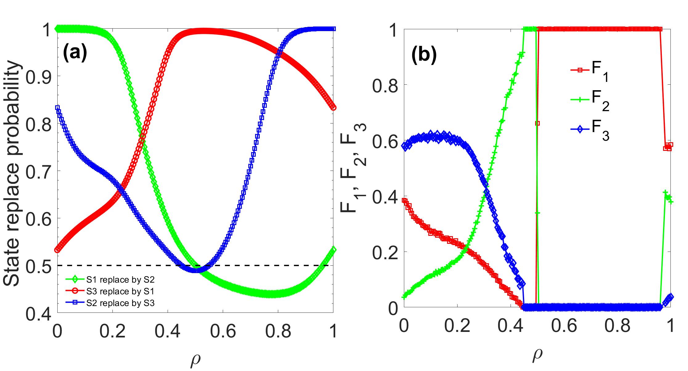
Figure 10: (Color online) Predictions of mean field/pair approximation theory. The replacement probability between any two types of agents and the frequency of every type of agents as predicted theoretically, where the latter is calculated from the mean field theory based on the former. (a) Theoretically predicted replacement probability based on the nine boundary structures in Fig. 8(b). Each point is the average value of the replacement probability from the nine boundary configurations. The green (light gray), red (medium gray), and blue (dark gray) curves are the probabilities of state $S^{(1)}$ replaced by $S^{(2)}$, of $S^{(3)}$ replaced by $S^{(1)}$, and of $S^{(2)}$ replaced by $S^{(3)}$, respectively. (b) The mean-field predicted frequency of every types of agents, where the red (medium gray), green (light gray), and blue (dark gray) curves are the frequencies of $S^{(1)}$, $S^{(2)}$, and $S^{(3)}$ type of agents, respectively, and every point is the average value of the last $500$ time steps of total $10000$ mean-field simulation steps. The incremental step in $\rho$ is $0.005$.

The pairwise interaction based picture suggests that the replacement probability $P_{S^{(x)}\rightarrow S^{(y)}}$ can in fact be regarded as an approximation of the strategy transformation probability on the square lattice. Figure 10(a) shows the interdependence between $P_{S^{(x)}\rightarrow S^{(y)}}$ and $\rho$, where $x,y\in[1,2,3]$. We see that, for $\rho<0.4$ (regions 1, 2, and 3), the values of $P_{S^{(1)}\rightarrow S^{(2)}}$, $P_{S^{(3)}\rightarrow S^{(1)}}$, and $P_{S^{(2)}\rightarrow S^{(3)}}$ are all above $0.5$, indicating the following RPS mechanism: $S^{(2)}$ excludes $S^{(1)}$, $S^{(1)}$ drives out $S^{(3)}$, and $S^{(3)}$ precludes $S^{(2)}$. For $0.495<\rho<0.96$, we have $P_{S^{(1)}\rightarrow S^{(2)}}<0.5$, which means $P_{S^{(2)}\rightarrow S^{(1)}}>0.5$, so $S^{(1)}$ actually ousts $S^{(2)}$ in this case. Since $P_{S^{(3)}\rightarrow S^{(1)}}\approx 1$, $S^{(1)}$ eliminates both $S^{(2)}$ and $S^{(3)}$, and this explains the dominance of $S^{(1)}$ in region 4. Our pair approximation method thus provides an understanding of the qualitative behavior of the system in a wide parameter range through local interactions.

IV.2 Mean-field theory

From a pairwise interaction based microscopic analysis of the replacement probability, the behaviors of the hypergame dynamics on a global scale can be understood quantitatively. In terms of the mean field theory, the frequencies of the three strategies in the system are governed by the following master equation

$$\frac{dF_{1}}{dt} = [{P_{S^{(2)}\rightarrow S^{(1)}}}-{P_{S^{(1)}\rightarrow S^{(2)}}}]\cdot F_{1}F_{2}$$

$$+ [{P_{S^{(3)}\rightarrow S^{(1)}}}-{P_{S^{(1)}\rightarrow S^{(3)}}}]\cdot F_{1}F_{3},$$

$$\frac{dF_{2}}{dt} = [{P_{S^{(1)}\rightarrow S^{(2)}}}-{P_{S^{(2)}\rightarrow S^{(1)}}}]\cdot F_{1}F_{2}$$

$$+ [{P_{S^{(3)}\rightarrow S^{(2)}}}-{P_{S^{(2)}\rightarrow S^{(3)}}}]\cdot F_{2}F_{3},$$

$$F_{3} = 1-F_{1}-F_{2},$$

where $F_{1}$, $F_{2}$, $F_{3}$ are the frequencies of $S^{(1)}$, $S^{(2)}$, and $S^{(3)}$, respectively. The numerical solution of the master equation group gives estimates of the frequencies of the three strategies. A comparison between Figs. 1 and 10(b) reveals that our mean-field calculation captures the essential dynamical behavior of the system in a wide range of parameter $\rho$ (regions 2 and 4 as well as the right side of region 1). For $\rho<0.445$, the behaviors of $F_{1}$, $F_{2}$, and $F_{3}$ from the mean-field theory coincide with the behavior of the real system in region 2, the RPS-like state, almost exactly. For $0.445<\rho<0.495$, the dominant behavior of $S^{(2)}$ is similar to that in the ending part of region 3. For $0.495<\rho<0.96$, the dominance of $S^{(1)}$ is well reproduced by the theory. For $\rho>0.96$, the numerically observed advantage of $S^{(2)}$ is reproduced. The transition points between the various regions are determined by the points where the probabilities $P_{S^{(x)}\rightarrow S^{(y)}}$ cross the line of $P_{S^{(x)}\rightarrow S^{(y)}}=0.5$ in Fig. 10(a) as $\rho$ increases, due to the flip over of the “predator-prey” relation between $S^{(x)}$ and $S^{(y)}$.

Our mean field theory fails to predict the behaviors in region 3, where the equilibrium state can be the absorption state of two strategies. There are two reasons for this: extremely long transient time and finite size effect. Firstly, to predict which strategy would take over according to the evolution pattern even after a very long simulation time (a typical transient time is $0.5\times 10^{6}$ time steps) is not feasible, since it is not possible to determine which strategy would die first when the number of critical time steps determining the fate of a strategy is negligibly small. Our numerical simulations show that, even if the frequency of one strategy, $S^{(1)}$ or $S^{(3)}$, approaches zero, revival at later time can occur with a high probability. Toward the right end of region 2, $F_{1}$ and $F_{3}$ are close to zero and, as $\rho$ is increased, there comes a point at which one of frequencies actually becomes zero so that the system enters into region 3. Secondly, calculations with different lattice sizes reveal that the absorption state emerges earlier in smaller lattices, and the critical $\rho$ value separating regions 2 and 3 increases with the lattice size. This implies that a finite-size effect plays the role of eliminating $S^{(1)}$ or $S^{(3)}$ to generate the one-strategy dominant state. Fluctuation effects are more severe in smaller lattices, so $S^{(1)}$ may become extinct or $S^{(1)}$ and $S^{(3)}$ clusters may be separated spatially with a higher probability.

V Discussion

In most existing works on evolutionary game dynamics on networks, a basic assumption is that the set of possible strategies is common to all players in the system Nowak and May (1992); Nowak et al. (1994); Ohtsuki et al. (2006); Taylor et al. (2007); Débarre et al. (2014); Allen et al. (2017). This assumption is reasonable for a variety of real-world phenomena and, in certain cases, makes possible a deep mathematical understanding of the game dynamics. The consideration motivating our work is that, in the real world, there can be situations where this assumption is not accurate. For example, in a social network, the individuals can have different backgrounds of knowledge, financial status, and experience. It is then conceivable that the strategy sets available to different players may not be identical. To investigate hypergame dynamics on networks is technically quite difficult, and such studies are still rare in the literature. We are led to consider the simplest setting of three available strategies with any player’s access to two (restrictively mixed-strategies). Even for the relatively simple setting, a mathematical treatment is not feasible: we thus rely on a combination of numerical computations and physical reasoning based on the pairwise interaction and mean field approximations to gain insights into evolutionary hypergame dynamics on regular networks.

We find a variety of dynamical behaviors and equilibrium states, including states in which most players use one strategy (one dominant strategy) and those where players use multiple strategies (coexisting strategies). There are parameter regions in which the equilibrium frequencies of the strategies are completely predictable (e.g., regions 1, 2, and 4 in Fig. 2), but there is also a region of unpredictability (region 3). We also uncover equilibrium states characteristic of those from cyclic competition dynamics, e.g., RPS-like states. A striking phenomenon is that, a nearly extinct strategy can revive and dominate the whole system. Qualitatively, this may be understood as a consequence of the unpredictability: in a parameter region where prediction of the system’s asymptotic state is ruled out, there can be transitions from the RPS-like state. In particular, starting from an RPS state, if the advantage of one strategy keeps growing and wins more and more agents, the living space of the other two strategies would be suppressed. At a certain point, the coverage of the two weak strategies would be so low that random fluctuations would remove one of them. If the remaining strategy is a prey of the strong strategy, the system would be dominated by the strong one. However, if the remaining strategy of the two weak ones is the prey of the extinct one, then regardless of its weakness, it would eventually overturn the entire population. A quantitative understanding of this phenomenon is lacking at the present.

We also find that, in hypergame of the prisoner’s dilemma type, self-organization of cooperation can be promoted. For example, as the parameter $\rho$ is increased, the probability of cooperation can increase monotonically and reaches the value of close to unity (Fig. 3). Comparing with the traditional prisoner’s dilemma game with loneliness Szabó and Hauert (2002), in our hypergame, it is not necessary for voluntary participation to create a cyclic dominance of strategies to promote cooperation.

Our work demonstrates that the diversity in the individuals’ understanding of the environmental strategies can play an important role in the evolution of strategy distribution on a global scale, and it can generate behaviors that are fundamentally different from those from the traditional explicit-strategy game dynamics. The basic parameter $\rho$ in our model, the probability of adopting a strategy, is key to generating the various complex dynamical behaviors. This parameter in fact measures the fraction of each pure strategy within the restrictively mixed strategy, whose changes drive the system into dramatically different equilibrium states. Our study reveals that a slight change in the fraction may completely overturn the relative advantage between the strategies, suggesting that the game dynamics can be manipulated through small changes in the parameter. This opens a door to controlling evolutionary hypergame dynamics.

References

- Szabó and Borsos (2016) G. Szabó and I. Borsos, Phys. Rep. 624, 2 (2016).
- Smith (1982) J. M. Smith, Evolution and the Theory of Games (Cambridge university press, Cambridge UK, 1982).
- Von Neumann and Morgenstern (2007) J. Von Neumann and O. Morgenstern, Theory of Games and Economic Behavior (Princeton university press, Princeton NJ, 2007).
- Colman (2013) A. M. Colman, Game Theory and Its Applications in the Social and Biological Sciences, 2nd ed. (Routledge Taylor and Francis Group, London, 2013).
- Smith and Price (1973) J. M. Smith and G. Price, Nature 246, 15 (1973).
- Hamilton and Axelrod (1981) W. D. Hamilton and R. Axelrod, Science 211, 1390 (1981).
- Dugatkin (1997) L. A. Dugatkin, BioScience 47, 355 (1997).
- J. L. Sachs et al. (2004) J. L. Sachs, U. G. Mueller, T. P. Wilcox, and J. J. Bull, Quart. Rev. Biol. 79, 135 (2004).
- Nowak (2006) M. A. Nowak, Science 314, 1560 (2006).
- Vukov et al. (2006) J. Vukov, G. Szabó, and A. Szolnoki, Phys. Rev. E 73, 067103 (2006).
- Szolnoki and Szabó (2007) A. Szolnoki and G. Szabó, Europhysics Letters 77, 30004 (2007).
- Nowak and May (1992) M. A. Nowak and R. M. May, Nature 359, 826 (1992).
- Nowak et al. (1994) M. A. Nowak, S. Bonhoeffer, and R. M. May, Proc. Nat. Acad. Sci. (USA) 91, 4877 (1994).
- Ohtsuki et al. (2006) H. Ohtsuki, C. Hauert, E. Lieberman, and M. A. Nowak, Nature 441, 502 (2006).
- Taylor et al. (2007) P. D. Taylor, T. Day, and G. Wild, Nature 447, 469 (2007).
- Débarre et al. (2014) F. Débarre, C. Hauert, and M. Doebeli, Nat. Commun. 5, 3409 (2014).
- Allen et al. (2017) B. Allen, G. Lippner, Y.-T.Chen, B. Fotouhi, N. Momeni, S.-T. Yau, and M. A. Nowak, Nature 544, 227 (2017).
- Sugden (1986) R. Sugden, The Economics of Rights Co-operation and Welfare (Blackwell, Oxford UK, 1986).
- Hardin (1968) G. Hardin, Science 162, 1243 (1968).
- Fehr and Gächter (2002) E. Fehr and S. Gächter, Nature 415, 137 (2002).
- Sicardi et al. (2009) E. A. Sicardi, H. Fort, M. Vainstein, and J. J. Arenzon, J. Theo. Biol. 256, 240 (2009).
- Wang et al. (2006) W.-X. Wang, J. Ren, G.-R. Chen, and B.-H. Wang, Phys. Rev. E 74, 056113 (2006).
- Hauert and Doebeli (2004) C. Hauert and M. Doebeli, Nature 428, 643 (2004).
- Szabó et al. (2005) G. Szabó, J. Vukov, and A. Szolnoki, Phys. Rev. E 72, 047107 (2005).
- Vukov et al. (2008) J. Vukov, G. Szabó, and A. Szolnoki, Phys. Rev. E 77, 026109 (2008).
- Helbing and Yu (2009) D. Helbing and W.-J. Yu, Proc. Nat. Acad. Sci. (USA) 106, 3680 (2009).
- Du et al. (2009) W.-B. Du, X.-B. Cao, M.-B. Hu, and W.-X. Wang, Europhys. Lett. 87, 60004 (2009).
- Santos et al. (2008) F. C. Santos, M. D. Santos, and J. M. Pacheco, Nature 454, 213 (2008).
- Chen et al. (2009) Y.-Z. Chen, Z.-G. Huang, S.-J. Wang, Y. Zhang, and Y.-H. Wang, Phys. Rev. E 79, 055101(R) (2009).
- Chen and Lai (2012) Y.-Z. Chen and Y.-C. Lai, Phys. Rev. E 86, 045101(R) (2012).
- May and Leonard (1975) R. M. May and W. J. Leonard, SIAM J. Appl. Math. 29, 243 (1975).
- Frean and Abraham (2001) M. Frean and E. R. Abraham, P. Roy. Soc. B-Biol. Sci. 268, 1323 (2001).
- Kerr et al. (2002) B. Kerr, M. A. Riley, M. W. Feldman, and B. J. Bohannan, Nature 418, 171 (2002).
- Szabó and Hauert (2002) G. Szabó and C. Hauert, Phys. Rev. Lett. 89, 118101 (2002).
- Semmann et al. (2003) D. Semmann, H.-J. Krambeck, and M. Milinski, Nature 425, 390 (2003).
- Reichenbach et al. (2007) T. Reichenbach, M. Mobilia, and E. Frey, Nature 448, 1046 (2007).
- Szabó and Fath (2007) G. Szabó and G. Fath, Phys. Rep. 446, 97 (2007).
- Reichenbach et al. (2008) T. Reichenbach, M. Mobilia, and E. Frey, J. Theor. Biology 254, 368 (2008).
- Berr et al. (2009) M. Berr, T. Reichenbach, M. Schottenloher, and E. Frey, Phys. Rev. Lett. 102, 048102 (2009).
- Wang et al. (2010) W.-X. Wang, Y.-C. Lai, and C. Grebogi, Phys. Rev. E 81, 046113 (2010).
- Shi et al. (2010) H. Shi, W.-X. Wang, R. Yang, and Y.-C. Lai, Phys. Rev. E 81, 030901 (2010).
- Yang et al. (2010) R. Yang, W.-X. Wang, Y.-C. Lai, and C. Grebogi, Chaos 20, 023113 (2010).
- Ni et al. (2010a) X. Ni, W.-X. Wang, Y.-C. Lai, and C. Grebogi, Phys. Rev. E 82, 066211 (2010a).
- Ni et al. (2010b) X. Ni, R. Yang, W.-X. Wang, Y.-C. Lai, and C. Grebogi, Chaos 20, 045116 (2010b).
- Wang et al. (2011) W.-X. Wang, X. Ni, Y.-C. Lai, and C. Grebogi, Phys. Rev. E 83, 011917 (2011).
- Jiang et al. (2012) L.-L. Jiang, W.-X. Wang, Y.-C. Lai, and X. Ni, Phys. Lett. A 376, 2292 (2012).
- Park et al. (2013) J. Park, Y. Do, Z.-G. Huang, and Y.-C. Lai, Chaos 23, 023128 (2013).
- Szabó and Sznaider (2004) G. Szabó and G. A. Sznaider, Phys. Rev. E 69, 031911 (2004).
- Peltomäki and Alava (2008) M. Peltomäki and M. Alava, Phys. Rev. E 78, 031906 (2008).
- Szabó et al. (2007) G. Szabó, A. Szolnoki, and G. A. Sznaider, Phys. Rev. E 76, 051921 (2007).
- Szabó and Szolnoki (2008) G. Szabó and A. Szolnoki, Phys. Rev. E 77, 011906 (2008).
- Avelino et al. (2012) P. Avelino, D. Bazeia, L. Losano, J. Menezes, and B. Oliveira, Phys. Rev. E 86, 036112 (2012).
- Vukov et al. (2013) J. Vukov, A. Szolnoki, and G. Szabó, Phys. Rev. E 88, 022123 (2013).
- Kang et al. (2013) Y. Kang, Q. Pan, X. Wang, and M. He, Physica A 392, 2652 (2013).
- Zheng et al. (2014) H.-Y. Zheng, N. Yao, Z.-G. Huang, J. Park, Y.-H. Do, and Y.-C. Lai, Sci. Rep. 4, 7486 (2014).
- Park et al. (2017) J.-P. Park, Y.-H. Do, B.-S. Jang, and Y.-C. Lai, Sci. Rep. 7, 7465 (2017).
- Szabó and Tőke (1998) G. Szabó and C. Tőke, Phys. Rev. E 58, 69 (1998).
- Hauert and Szabó (2005) C. Hauert and G. Szabó, Am. J. Phys 73, 405 (2005).
- Bennett (1977) P. G. Bennett, Omega 5, 749 (1977).
- Gharesifard and Cortés (2012) B. Gharesifard and J. Cortés, IEEE Trans. Automat. Contr. 57, 1627 (2012).
- Sasaki and Kijima (2012) Y. Sasaki and K. Kijima, J. Syst. Sci. Complex. 25, 720 (2012).
- Kovach et al. (2015) N. S. Kovach, A. S. Gibson, and G. B. Lamont, Game Theo. 2015, 570639 (2015).
- Nowak and May (1993) M. A. Nowak and R. M. May, Int. J. Bifur. chaos 3, 35 (1993).
- (64) Supplementary movies: examples of time evolution of hypergame dynamics .
- Wu and Wang (2007) Z.-X. Wu and Y.-H. Wang, Phys. Rev. E 75, 041114 (2007).
- Perc and Marhl (2006) M. Perc and M. Marhl, New J. Phys. 8, 142 (2006).
- Gleeson (2013) J. P. Gleeson, Phys. Rev. X 3, 021004 (2013).