Model Hamiltonian for strongly correlated systems: Systematic, self-consistent, and unique construction

Abstract

An interacting lattice model describing the subspace spanned by a set of strongly correlated bands is rigorously coupled to density functional theory to enable ab initio calculations of geometric and topological material properties. The strongly correlated subspace is identified from the occupation number band structure as opposed to a mean-field energy band structure. The self-consistent solution of the many-body model Hamiltonian and a generalized Kohn-Sham equation exactly incorporates momentum-dependent and crystal-symmetric correlations into electronic structure calculations in a way that does not rely on a separation of energy scales. Calculations for a multiorbital Hubbard model demonstrate that the theory accurately reproduces the many-body macroscopic polarization.

I Introduction

Predicting electronic properties of strongly correlated materials is an enduring challenge in condensed matter physics. Homogeneous electron gas based semilocal density functional approximations do not capture the strong correlations between electrons hopping within a manifold of localized states, as present in Mott insulators Mott (1949, 1964); Brandow (1977); Imada et al. (1998), cuprate superconductors Anderson (1987); Monthoux et al. (1991); Dagotto (1994); Lee et al. (2006); Schrieffer and Brooks (2007) and heavy-fermion compounds Stewart (1984); Freeman et al. (1987); Fuggle et al. (1988); Grewe and Steglich (1991); Hewson (1997). While progress has been made, there remains a need for ab initio computational methods capable of accurately predicting the emergent phenomena, phase diagrams and sensitive dependence on external parameters in such systems.

Density functional theory (DFT) calculations of correlated solids may encounter two types of deficiencies. First, a calculation may deliver a qualitatively incorrect density or total energy. By virtue of the Hohenberg-Kohn theorem Hohenberg and Kohn (1964), these two quantities should be correct if the exchange-correlation functional is accurate. The inability of semilocal approximations to correctly predict orbital ordering in some compounds, e.g., KCuF₃ Liechtenstein et al. (1995); Towler et al. (1995); Pavarini et al. (2008); Leonov et al. (2010), LaMnO₃ Elfimov et al. (1999); Yin et al. (2006); Pavarini and Koch (2010); Leonov et al. (2010), and KCrF₃ Autieri et al. (2014); Novoselov et al. (2016), implies that not only the densities and energies but also the structures are incorrect, since they lack the associated symmetry-lowering Jahn-Teller distortion. Similarly, spin-DFT von Barth and Hedin (1972); Gunnarsson and Lundqvist (1976) calculations of the spin state or pressure-induced spin state crossover in transition metal atoms in oxides Cohen et al. (1997) may fail qualitatively, or suffer from large uncertainties, as seen for Fe in MgO Korotin et al. (1994); Tsuchiya et al. (2006) and MgSiO₃ Zhang and Oganov (2006); Umemoto et al. (2008); Hsu et al. (2010).

A second type of deficiency occurs when the Kohn-Sham system Kohn and Sham (1965), an auxiliary noninteracting system that reproduces the density of the interacting system, does not provide a qualitatively correct reference state for subsequent higher-level calculations. In the absence of spin-symmetry breaking, Kohn-Sham band structures are metallic for Mott insulators and as such do not provide an appropriate reference state for calculations of the macroscopic polarization and related quantities. An important unsolved problem is to find a way to perform accurate ab initio calculations of topological invariants in strongly correlated systems. Topological invariants were originally formulated in terms of the Bloch states of a mean-field band structure Thouless et al. (1982); Haldane (1988); Kane and Mele (2005); Fu et al. (2007); Bernevig et al. (2006); Moore and Balents (2007); Roy (2009), almost invariably the Kohn-Sham band structure, an approach that may give incorrect results in strongly correlated systems. Although interacting topological invariants can be rigorously defined in terms of the Berry curvature of the correlated many-body wavefunction Thouless (1983); Niu and Thouless (1984), those formulas have not been applied in ab initio calculations of real materials due to the formidable difficulty of approximating the correlated wavefunction of an infinite solid. The mean-field-based geometric phase formula for the macroscopic polarization King-Smith and Vanderbilt (1993); Resta (1994) has been similarly generalized to interacting systems Ortiz and Martin (1994), but the latter formula has not been applied to real materials for the same reason.

To study the phases and physical properties of strongly correlated materials, one typically introduces an effective Hamiltonian defined on a lattice and comprising a small but relevant subset of low-energy degrees of freedom. Thus, the single narrow band in the Hubbard model Hubbard (1963); Kanamori (1963); Gutzwiller (1963); Anderson (1959) represents the Mott insulator-metal transition in transition metal oxides, while the coexistence of localized and itinerant electrons in the periodic Kondo and Anderson models Doniach (1977); Tsunetsugu et al. (1997); Hewson (1997) embodies the key physics of heavy fermion compounds. At this level of theory, the interaction between high-energy and low-energy degrees of freedom is one-way: the coupling to high-energy states is assumed to renormalize the parameters of the low-energy Hamiltonian, but the effects of many-body quantum fluctuations within the correlated low-energy sector on the high-energy degrees of freedom are neglected. Effective low-energy models can be rigorously derived by a procedure called downfolding Löwdin (1951, 1962); Brandow (1979).

The downsides of model Hamiltonian approaches are ambiguities in the choice of the model and uncertainties in the model parameters. Quantitative results depend on the precise values of the model parameters, which are often estimated from ab initio calculations or fixed empirically by comparison with experiment. Empirical approaches have limited predictive power, and often there are more relevant parameters than could conceivably be determined by fitting to experiment. DFT has long been used to guide the choice of the relevant orbital, spin, and lattice degrees of freedom to be included in a model Hamiltonian and to estimate their mutual interactions. The one-body hopping and on-site potential terms of approximate tight-binding models are routinely derived by fitting Papaconstantopoulos (1986); Horsfield and Bratkovsky (2000); Papaconstantopoulos and Mehl (2003) Kohn-Sham band structures with Slater-Koster parameters Slater and Koster (1954) or by transforming the Kohn-Sham Hamiltonian from the basis of Bloch states to a basis of localized (Wannier) functions Andersen and Jepsen (1984); Mattheiss and Hamann (1989); McMahan et al. (1990); Marzari and Vanderbilt (1997); Ku et al. (2002).

The definition of two-body interaction parameters, on the other hand, is fraught with difficulty. The largest Coulomb matrix element is the Hubbard interaction $U$ between two electrons occupying the same atomic-like (e.g. $d$ or $f$) orbital. The definition $U=E(d^{n+1})+E(d^{n-1})-2E(d^{n})$ Vleck (1953) in terms of atomic configurations with different numbers of localized $d$ electrons self-consistently screened by conduction electrons Herring (1966) agrees well with photoemission spectra for very localized orbitals, such as the $4f$ orbitals in rare-earth metals Herbst et al. (1978), but still needs to be rigorously connected to an interaction term $U\hat{n}_{i\uparrow}\hat{n}_{i\downarrow}$ in a model Hamiltonian. If one associates a localized Wannier function $w_{i}(\mathbf{r})=w(\mathbf{r}-\mathbf{R}_{i})$ to the lattice site $i$ of a model Hamiltonian, then it is natural to define $U$ as the on-site matrix element of the Coulomb interaction, $U=\langle w_{i}w_{i}|V_{ee}|w_{i}w_{i}\rangle$ Anderson (1959, 1961); Hubbard (1963). However, this gives unrealistically large values, since the bare Coulomb interaction $V_{ee}(\mathbf{r},\mathbf{r}^{\prime})=e^{2}/|\mathbf{r}-\mathbf{r}^{\prime}|$ should be screened Anisimov et al. (1997a); Springer and Aryasetiawan (1998); Kotani (2000); Biermann et al. (2003). Interatomic and interorbital Coulomb matrix elements are usually not negligible and, if not included in the model Hamiltonian, contribute to further renormalizing the value of $U$ Gunnarsson and Schönhammer (1989); Gunnarsson (1990). Screening is accounted for in the constrained random phase approximation Aryasetiawan et al. (2004); Miyake et al. (2009); Vaugier et al. (2012), where Coulomb matrix elements are defined as $U_{ijkl}=\langle w_{i}w_{j}|\epsilon^{-1}V_{ee}|w_{k}w_{l}\rangle$. The dielectric function $\epsilon$ is calculated from an ab initio irreducible electronic polarizability in which the contribution from a low-energy correlated subspace has been subtracted out to avoid double-counting screening channels that are already present in the many-body model. Since the width and shape of conventional Wannier functions depend on the gauge of the Bloch functions from which they are constructed, the $U_{ijkl}$ determined in this way are dependent on the specific gauge choices that are made.

The constrained occupation method in DFT provides a seamless estimate of effective interaction parameters by relating them to how the energy changes in response to changes in the occupation or magnetic moment of a local orbital Dederichs et al. (1984); Min et al. (1986); McMahan et al. (1988); Gunnarsson et al. (1989); Hybertsen et al. (1989). Although the effective $U$ is thus calculated self-consistently in the presence of all screening channels and with only the information contained in the exchange-correlation functional, it still depends on the arbitrary definition of the local orbital whose occupation is to be constrained. All existing approaches to the calculation of model parameters suffer from this fundamental nonuniqueness. Even the one-body terms evaluated in Wannier-based tight-binding approaches are not unambiguously defined, as the hopping amplitudes depend implicitly on the many-body configuration of the relevant local orbitals Gunnarsson and Jepsen (1988); Gunnarsson et al. (1989) and should be renormalized by Coulomb interactions Gunnarsson and Schönhammer (1989).

A general procedure for deriving effective low-energy models is to integrate out the high-energy degrees of freedom. The Hamiltonian for the high-energy sector and the interaction terms that couple the high-energy and low-energy sectors are “downfolded” Löwdin (1951, 1962); Brandow (1979) into an effective operator that acts on the low-energy Hilbert space, thus defining an effective low-energy model with renormalized Hamiltonian parameters Gunnarsson (1990); Andersen et al. (1995). This strategy has developed into a widely used ab initio downfolding method Lichtenstein and Katsnelson (1998); Aryasetiawan et al. (2004); Solovyev and Imada (2005); Solovyev (2008); Miyake and Aryasetiawan (2008); Aryasetiawan et al. (2009); Miyake et al. (2009); Imada and Miyake (2010); Vaugier et al. (2012); Casula et al. (2012); E. $\c{S}$aşıoglu et al. (2013); Hirayama et al. (2013, 2017); Nilsson and Aryasetiawan (2018). After defining an energy window for the construction of localized Wannier functions and choosing a correlated subspace spanned by Wannier functions of specific orbital character, the frequency-dependent interaction parameters of an effective low-energy model are calculated by applying the constrained random phase approximation to the disentangled band structure. The effective low-energy model depends on the number and character of the Wannier orbitals in the correlated subspace, as well as the energy window and gauge choices used in constructing the Wannier functions Vaugier et al. (2012); Miyake et al. (2009).

Downfolding methods are justified when there is a separation of energy scales. In ab initio downfolding methods, the separation into low- and high-energy subspaces, as well as the definition of the Wannier orbital basis for the many-body model, are based on the mean-field Kohn-Sham band structure. The low-energy localized Wannier orbitals are chosen as the degrees of freedom to be correlated at a higher level of theory by solving the many-body model Miyake et al. (2009); Vaugier et al. (2012); Hirayama et al. (2017). Another approach to downfolding is to start from an ab initio quantum Monte Carlo calculation and use a fitting procedure to determine the effective Hamiltonian that best reproduces the two-body reduced density matrix in a low-energy sector Changlani et al. (2015).

Many materials of current interest have complex multiband character with several competing interactions, involving charge, spin, orbital and lattice degrees of freedom, making it hard to arrive at a unique model Hamiltonian. In several cases, multiple different models have been introduced to describe the same material property; for example, one-band Anderson (1987); Zhang and Rice (1988) and three-band Emery (1987); Varma et al. (1987); Abrahams et al. (1987); Hirsch (1987) extended Hubbard models for high $T_{c}$ cuprate superconductors with parameters estimated early on from DFT band structure calculations Mattheiss (1987); Yu et al. (1987); McMahan et al. (1988); Hybertsen et al. (1989); Mattheiss and Hamann (1989); Pickett (1989); McMahan et al. (1990); Andersen et al. (1995); a Kane-Mele-type model Shitade et al. (2009) and a Kitaev-Heisenberg model Jackeli and Khaliullin (2009); Chaloupka et al. (2010) with a raft of additional interactions Kimchi and You (2011); Albuquerque et al. (2011); Choi and et al. (2012); Singh et al. (2012); Ye et al. (2012); Chaloupka et al. (2013); Rau et al. (2014); Bhattacharjee et al. (2012); Sizyuk et al. (2014); Winter et al. (2016); Laubach et al. (2017) for sodium iridate (Na₂IrO₃) and its zigzag spin ordering Liu et al. (2011); Choi and et al. (2012); Ye et al. (2012), which has also been studied with first-principles calculations Foyevtsova et al. (2013); Yamaji et al. (2014); Katukuri and et al. (2014); Hu et al. (2015); one-band Perfetti et al. (2005, 2006); Sipos et al. (2008); Lahoud et al. (2014) and multiband Qiao and et al. (2017) Hubbard models, possibly with additional interlayer coupling Bovet et al. (2003); Ritschel et al. (2015), spin-orbit coupling Rossnagel and Smith (2006), disorder Di Salvo et al. (1975); Mutka et al. (1981); Zwick et al. (1998); Lahoud et al. (2014) and Hubbard-Holstein renormalization Cho et al. (2015) effects, for the Mott Tosatti and Fazekas (1976); Fazekas and Tosatti (1979) and superconducting Morosan et al. (2006); Sipos et al. (2008); Ang et al. (2013) phases in the charge density wave state Wilson et al. (1975); Scruby et al. (1975) of the transition metal dichalcogenide 1$T$-TaS₂. The challenges one faces in defining a unique model Hamiltonian make it difficult to reach agreement on the underlying physical explanation for the observed phases and emergent phenomena, particularly for cuprate superconductors, where various issues have been debated for decades Zaanen and et al. (2006). Does every material have a model Hamiltonian that is unique in some well-defined sense for a chosen subset of variables?

While DFT is the standard framework for itinerant, nearly free-electron-like states and model Hamiltonians are widely used for strongly correlated localized states, both approaches have limitations when local and itinerant electrons coexist. The advantages of treating localized and itinerant electrons differently was appreciated long ago in the works of Anderson, Hubbard, Kanamori, Gutzwiller and others Anderson (1959, 1961); Hubbard (1963); Kanamori (1963); Gutzwiller (1963). Several methods that combine model Hamiltonians with DFT have since been developed. Most approaches involve a mapping to an auxiliary Anderson impurity model, i.e. they single out an atomic-like orbital with strong on-site interactions and treat it as an impurity that hybridizes with a band of noninteracting electrons representing the remaining delocalized degrees of freedom of the solid. In DFT+dynamical mean field theory (DFT+DMFT) Anisimov et al. (1997b); Lichtenstein and Katsnelson (1998); Kotliar et al. (2006); Held et al. (2006), the frequency-dependent hybridization function of the Anderson impurity model is determined by requiring self-consistency between the local lattice Green’s function calculated within DFT and the impurity Green’s function of the Anderson model. In the DFT+numerical renormalization group (DFT+NRG) approach Lucignano et al. (2009); Baruselli et al. (2012, 2013); Requist et al. (2014); Baruselli et al. (2015), frequency-independent impurity model parameters are determined by equating the mean-field scattering phase shifts of the Anderson model to the scattering phase shifts calculated within DFT. In density matrix embedding theory (DMET), the Schmidt decomposition between a few localized states and the rest of the system leads to an effective Anderson model in which the frequency-independent coupling to bath states is determined by imposing self-consistency on the local reduced density matrix Knizia and Chan (2012). In site occupation embedding theory fromager2015; senjean2017, one solves self-consistently for the site occupation numbers of a lattice model, with Hubbard interactions turned on only in a fragment consisting of a few sites, in the presence of an embedding potential derived from a bath correlation energy functional.

By limiting correlations to the impurity model subspace, DFT+DMFT and all impurity-based embedding approaches explicitly break lattice translational symmetry in the correlated part of the problem. As a result, they do not provide information on nonlocal momentum-dependent correlations. This will cause inaccuracies in the calculation of geometric and topological quantities, which are specifically related to the $\mathbf{k}$-dependence of the single-particle Bloch functions in the mean-field case and the total quasimomentum-dependence of the correlated wavefunction in the interacting case. Geometric and topological properties are therefore sensitive to the momentum-dependence of two-body correlations in strongly correlated systems.

In this article, we propose an ab initio theory that rigorously couples DFT to a unique many-body lattice model. The strongly correlated subspace described by the lattice model is chosen by selecting a subset of natural occupation number bands ($\mathbf{k}$-dependent eigenvalues of the one-body reduced density matrix) that are isolated from all others. Since natural occupation number bands are intrinsic variables directly calculable from the many-body wave function without the introduction of auxiliary mean-field quantities, they may provide a more accurate partitioning into strongly and weakly correlated subspaces than a partitioning based on mean-field energy bands. The one-body reduced density matrix is invariant with respect to the symmetry group of the crystal, and therefore its eigenfunctions, called natural Bloch orbitals, transform exactly as mean-field Bloch functions do and can be labeled by a wavevector $\mathbf{k}$ that is an element of the true Brillouin zone of the crystal. The many-body model Hamiltonian expressed in the subspace of strongly correlated natural Bloch orbitals therefore preserves lattice translational symmetry and all other symmetries of the crystal. Since the Hamiltonian model parameters are frequency independent, the many-body problem can be solved more efficiently than models with frequency-dependent parameters, for which a Lagrangian formalism is necessary. The lack of frequency dependence is an exact feature of the theory and does not imply that dynamical correlations are neglected.

Our theory provides a practical way to make ab initio calculations of geometric and topological properties in strongly correlated systems. It has recently been shown that the natural Bloch orbitals, natural occupation numbers and their conjugate phases, which combine to form a set of natural orbital geometric phases, contain most of the information about the effects of many-body correlations on geometric and topological quantities in the Rice-Mele-Hubbard model Requist and Gross (2018). Since these variables are included in our theory through the self-consistent solution of the many-body lattice model and a generalized Kohn-Sham equation, we expect to obtain accurate results for geometric and topological quantities in real systems. These quantities can be problematic in standard DFT. For example, the King-Smith–Vanderbilt formula King-Smith and Vanderbilt (1993) for the macroscopic polarization is undefined for Mott insulators and other systems for which the Kohn-Sham system is metallic. Calculating topological invariants in terms of mean-field Bloch states is similarly problematic, since it is only by neglecting the interaction-induced broadening of the mean-field band structure that one obtains a quantized result. In contrast, the natural occupation numbers form exact, unbroadened bands irrespective of the interaction strength. Hence, topological invariants calculated in terms of the natural Bloch orbitals are precisely quantized Requist and Gross (2018). Quantum Monte Carlo methods have been used to evaluate many-body topological invariants in correlated model systems Hohenadler and Assaad (2013). Although the application of such many-body methods to real systems with all electronic degrees of freedom is computationally prohibitive, they could be used instead of exact diagonalization to solve the model Hamiltonian in our theory, which self-consistently retains all electronic degrees of freedom in a generalized DFT framework.

Our main results from numerical calculations for a two-orbital Hubbard model are (i) a demonstration that two strongly correlated natural occupation number bands split off from the weakly correlated bands as the on-site interaction $U$ increases and (ii) a demonstration that our theory accurately predicts the many-body macroscopic polarization in strongly, weakly and intermediately correlated regimes of the model.

The article is organized as follows. In Sec. II, we present the fundamentals of the theory. In Sec. III, we define the two-orbital Hubbard model for which all calculations are made. In Sec. IV, we calculate the exact natural occupation number band structure and demonstrate the partitioning into weakly and strongly correlated bands. In Sec. V, we evaluate the model Hamiltonian for the strongly correlated bands and investigate its density dependence. In Sec. VI, we calculate the many-body polarization and verify that it is given correctly in our theory. We provide conclusions and an outlook on future challenges in Sec. VII.

II Theory

Our theory is based on the idea of partitioning the natural occupation number bands into weakly and strongly correlated subsets and treating the latter at a higher level of theory. To define the natural occupation number bands, we first need the one-body reduced density matrix

$$\rho_{1,\sigma\sigma^{\prime}}(\mathbf{r},\mathbf{r}^{\prime})=\mathrm{Tr}\big{[}\hat{\psi}_{\sigma^{\prime}}^{{\dagger}}(\mathbf{r}^{\prime})\hat{\psi}_{\sigma}(\mathbf{r})\,\hat{\rho}\big{]}{,}$$ (1)

where $\hat{\psi}_{\sigma}^{{\dagger}}(\mathbf{r})$ and $\hat{\psi}_{\sigma}(\mathbf{r})$ are the electronic creation and annihilation operators and $\hat{\rho}=\sum_{N,\alpha}w_{N\alpha}|\Psi_{N\alpha}\rangle\langle\Psi_{N\alpha}|$ is the density matrix of the system, which at equilibrium is an ensemble of $N$-electron eigenstates with weights $w_{N\alpha}=\exp[-\beta(E_{N\alpha}-\mu N)]/\sum_{N\alpha}\exp[-\beta(E_{N\alpha}-\mu N)]$. Our theory is formulated in the grand canonical ensemble for a system with temperature $\tau$ ($\beta=1/k_{B}\tau$) and chemical potential $\mu$. Since $\hat{\rho}_{1}$ commutes with lattice translations $\hat{T}_{\mathbf{a}}$, its eigenfunctions, which we call natural Bloch orbitals $\phi_{n\mathbf{k}}(\mathbf{r})$, obey the Bloch condition $\phi_{n\mathbf{k}}(\mathbf{r}+\mathbf{a})=e^{i\mathbf{k}\cdot\mathbf{a}}\phi_{n\mathbf{k}}(\mathbf{r})$ and can be labeled by a band index $n$, a wavevector $\mathbf{k}$, and other possible quantum numbers associated with the crystallographic space group. The natural Bloch orbitals are spin-orbitals, or generally two-component spinors $\phi_{n\mathbf{k}}(\mathbf{r})=\{\phi_{n\mathbf{k}\uparrow}(\mathbf{r}),\phi_{n\mathbf{k}\downarrow}(\mathbf{r})\}$, determined by the eigenvalue equation

$$\sum_{\sigma^{\prime}}\int\rho_{1\sigma\sigma^{\prime}}(\mathbf{r},\mathbf{r}^{\prime})\phi_{n\mathbf{k}\sigma^{\prime}}(\mathbf{r}^{\prime})d\mathbf{r}^{\prime}=f_{n\mathbf{k}}\phi_{n\mathbf{k}\sigma}(\mathbf{r}){.}$$ (2)

The occupation numbers $f_{n\mathbf{k}}$ form bands in the Brillouin zone of the crystal Requist and Gross (2018). In our theory, these natural occupation number bands take the place of mean-field energy bands. Bands whose occupation numbers differ significantly from 0 and 1, if present, will be called strongly correlated, and the remaining bands whose occupation numbers are close to 0 or 1 will be called weakly correlated. The natural Bloch orbitals are correspondingly partitioned into weakly and strongly correlated sets $\mathcal{S}$ and $\mathcal{D}$. In DFT, only a finite number of energy bands are occupied at $\tau=0$. In contrast, there are generally an infinite number of nonvanishing natural occupation number bands even at $\tau=0$, due to many-body correlations. If the $f_{n\mathbf{k}}$ are ordered in a nonincreasing sequence $f_{1\mathbf{k}},f_{2\mathbf{k}},\ldots$ for each $\mathbf{k}$, there will not generally exist a lower bound $b_{\mathbf{k}}>0$ such that $f_{n\mathbf{k}}\geq b_{\mathbf{k}}\;\forall n$; zero is an accumulation point of the spectrum.

Since there have been no many-body calculations of the natural occupation number bands in real materials, the extent to which they can be unambiguously partitioned into weakly and strongly correlated subsets is presently unknown. Our numerically exact results for a two-orbital Hubbard model (Fig. 2) provide a concrete example of a system where two strongly correlated bands clearly split off from the remaining two weakly correlated bands as the Hubbard interaction is increased. The distinction between weakly and strongly correlated bands is only an approximate notion, e.g. if one occupation number band hovers around 0.98 and another around 0.99, it would hardly be possible to argue that the former is more correlated than the latter. Moreover, if a band whose occupation numbers differ significantly from 0 and 1 in some region of the Brillouin zone has symmetry-enforced or accidental intersections with weakly correlated bands or is otherwise strongly “entangled” with them, it might be questionable to single it out for special treatment. Nevertheless, our theory is formally exact (in the DFT sense of returning the exact equilibrium values of the functional variables) for any partitioning of the occupation number bands. Specifically, if none of the bands are treated as strongly correlated, then our theory reduces to DFT (or current-DFT Vignale and Rasolt (1987)). On the other hand, if all of the bands are treated as strongly correlated, then the model Hamiltonian is simply the full many-body Hamiltonian expressed in the basis of natural Bloch orbitals. For real strongly correlated materials, where a few relevant bands would be treated at the full many-body level, we expect that it will be easier to find accurate functional approximations in our theory than in conventional DFT.

Even in cases where it is not possible to cleanly disentangle the bands, there may still be advantages to using the natural Bloch orbitals or natural Wannier functions Requist and Gross (2018), as opposed to mean-field Bloch orbitals or mean-field Wannier functions, in selecting a subset of degrees of freedom to treat at a higher level of theory. Natural Bloch orbitals are intrinsic variables of the system, being defined in terms of the one-body reduced density matrix, a quantity obtained by simply tracing out degrees of freedom—a linear operation—and may therefore provide a more suitable starting point than mean-field Bloch orbitals in strongly correlated systems.

The next step is to introduce a generalized density functional theory in which the basic variables are the density $n(\mathbf{r})$, the paramagnetic current density $\mathbf{j}_{p}(\mathbf{r})$, and the strongly correlated natural Bloch orbitals $\phi_{d\mathbf{k}\sigma}(\mathbf{r})$. The paramagnetic current density is included to correctly account for the coupling to an artificial vector potential that will be introduced to evaluate the macroscopic polarization, yet we expect that the $\mathbf{j}_{p}(\mathbf{r})$-dependence of the functionals can be neglected as a first approximation. As we are working at temperature $\tau$ and chemical potential $\mu$, we define the following grand potential functional for a system of interacting electrons in the presence of scalar and vector potentials $v(\mathbf{r})$ and $\mathbf{A}(\mathbf{r})$ (a uniform $\mathbf{A}$ is sufficient for our purposes ) Mermin (1965):

$$\Omega[n,\mathbf{j}_{p},\phi_{d\mathbf{k}},f_{d\mathbf{k}},\rho_{2}^{d}] =\int[v(\mathbf{r})-\mu]n(\mathbf{r})d\mathbf{r}$$

$$\quad+\frac{e}{c}\int\mathbf{A}(\mathbf{r})\cdot\mathbf{j}_{p}(\mathbf{r})d\mathbf{r}$$

$$\quad+\frac{e^{2}}{2mc^{2}}\int|\mathbf{A}(\mathbf{r})|^{2}n(\mathbf{r})d\mathbf{r}$$

$$\quad+F[n,\mathbf{j}_{p},\phi_{d\mathbf{k}},f_{d\mathbf{k}},\rho_{2}^{d}]{,}$$ (3)

where the universal functional $F$ is defined by the following constrained search Levy (1979) over density matrices $\rho$ that yield the set of variables $X=(n,\mathbf{j}_{p},\phi_{d\mathbf{k}},f_{d\mathbf{k}},\rho_{2}^{d})$:

$$F[n,\mathbf{j}_{p},\phi_{d\mathbf{k}},f_{d\mathbf{k}},\rho_{2}^{d}]=\min_{\rho\rightarrow X}\mathrm{Tr}[(\hat{T}+\hat{V}_{ee}-\tau\hat{S})\hat{\rho}]{,}$$ (4)

where $\hat{T}$ is the kinetic energy, $\hat{V}_{ee}$ is the electron-electron interaction, and $\hat{S}=-k_{B}\ln\hat{\rho}$ is the entropy operator. The functionals $\Omega$ and $F$ additionally depend on the natural occupation numbers $f_{d\mathbf{k}}$ and the two-body reduced density matrix $\rho_{2}^{d}$ in the strongly correlated $\mathcal{D}$ subspace. The matrix elements of $\rho_{2}^{d}$ are

$$(\rho^{d}_{2})_{121^{\prime}2^{\prime}} =\frac{1}{2}\mathrm{Tr}(c_{2^{\prime}}^{{\dagger}}c_{1^{\prime}}^{{\dagger}}c_{1}c_{2}\,\hat{\rho}){,}$$ (5)

where $1=(d_{1}\mathbf{k}_{1})$ and $c_{1}^{{\dagger}}$ is the creation operator for an electron in the natural Bloch orbital state $\phi_{d_{1}\mathbf{k}_{1}}\in\mathcal{D}$. The grand potential can be further decomposed by defining a kinetic-energy-entropy functional for noninteracting electrons (with $\hat{S}_{s}=-k_{B}\ln\hat{\rho}_{s}$)

$$K_{s}[n,\mathbf{j}_{p},\phi_{d\mathbf{k}},f_{d\mathbf{k}}] =\min_{\rho_{s}\rightarrow(n,\mathbf{j}_{p},\phi_{d\mathbf{k}},f_{d\mathbf{k}})}\mathrm{Tr}[(\hat{T}-\tau\hat{S}_{s})\hat{\rho}_{s}]$$ (6)

and a Hartree-exchange-correlation grand potential

$$\Omega_{hxc}[n,\mathbf{j}_{p},\phi_{d\mathbf{k}},f_{d\mathbf{k}},\rho_{2}^{d}] =F[n,\mathbf{j}_{p},\phi_{d\mathbf{k}},f_{d\mathbf{k}},\rho_{2}^{d}]$$

$$\quad-K_{s}[n,\mathbf{j}_{p},\phi_{d\mathbf{k}},f_{d\mathbf{k}}]{.}$$ (7)

The kinetic-energy-entropy functional $K_{s}[n,\mathbf{j}_{p},\phi_{d\mathbf{k}},f_{d\mathbf{k}}]$, defined by a constrained search over ensembles of Slater determinants $\rho_{s}$, is intermediate between the corresponding functionals in DFT Pittalis et al. (2011) and reduced density matrix functional theory Baldsiefen et al. (2015). Since $K_{s}[n,\mathbf{j}_{p},\phi_{d\mathbf{k}},f_{d\mathbf{k}}]$ accounts for the fractional occupation numbers of the strongly correlated natural Bloch orbitals, we expect it to provide a better approximation to the true kinetic-energy-entropy than the DFT functional. $\Omega$ and $F$ are defined on the domain of $(n,\mathbf{j}_{p},\phi_{d\mathbf{k}},f_{d\mathbf{k}},\rho_{2}^{d})$ that can be obtained from a fermionic density matrix, which we denote as the ensemble representable (ER) domain in analogy to the ensemble $N$ representable domain for fixed particle number $N$ Coleman (1963). Using the quantum generalization of Gibb’s variational principle for ensembles Mermin (1965), it is straightforward to prove the following variational principle.

Theorem.— The grand potential functional satisfies $\Omega[n,\mathbf{j}_{p},\phi_{d\mathbf{k}},f_{d\mathbf{k}},\rho_{2}^{d}]>\Omega_{0}$ for any $(n,\mathbf{j}_{p},\phi_{d\mathbf{k}},f_{d\mathbf{k}},\rho_{2}^{d})$ that are not equal to the correct equilibrium variables $(n_{0},\mathbf{j}_{p0},\phi_{d\mathbf{k}0},f_{d\mathbf{k}0},\rho^{d}_{20})$ yielding the potential $\Omega_{0}$.

The density and paramagnetic current density can be expressed in terms of the natural Bloch orbitals as

$$n(\mathbf{r}) =\sum_{n\mathbf{k}\sigma}f_{n\mathbf{k}}|\phi_{n\mathbf{k}\sigma}(\mathbf{r})|^{2}$$

$$\mathbf{j}_{p}(\mathbf{r}) =\frac{\hbar}{m}\mathrm{Im}\sum_{n\mathbf{k}\sigma}f_{n\mathbf{k}}\phi_{n\mathbf{k}\sigma}^{*}(\mathbf{r})\nabla\phi_{n\mathbf{k}\sigma}(\mathbf{r}){.}$$ (8)

Our strategy is now to postulate that a semilocal density functional Kohn and Sham (1965); von Barth and Hedin (1972); Perdew et al. (1996) provides a sufficiently accurate description of the weakly correlated bands in the sense that their contribution to the density in Eq. (8) can be well-approximated by a sum $\sum_{\sigma,n\mathbf{k}\in\mathcal{S}}g_{n\mathbf{k}}|\chi_{n\mathbf{k}\sigma}(\mathbf{r})|^{2}$ over KS-like Bloch orbitals $\chi_{n\mathbf{k}\sigma}(\mathbf{r})$ that are eigenstates of a noninteracting Hamiltonian with a scalar multiplicative potential $v_{s}(\mathbf{r})$. The thermal occupation numbers in this sum, $g_{n\mathbf{k}}=(1+\exp[\beta(\epsilon_{n\mathbf{k}}-\mu)])^{-1}$, follow the Fermi-Dirac distribution and therefore manifest thermal fluctuations but not quantum fluctuations. At the same time, we retain the fractional occupation numbers $f_{d\mathbf{k}}$ of the strongly correlated natural Bloch orbitals $\phi_{d\mathbf{k}}(\mathbf{r})$ as variational parameters, since they do exhibit significant quantum fluctuations.

The grand potential is minimized in an iterative fashion. First, for fixed $(f_{d\mathbf{k}},\rho_{2}^{d})$, $\Omega$ is minimized with respect to $n(\mathbf{r})$, $\mathbf{j}_{p}(\mathbf{r})$, and $\phi_{d\mathbf{k}\sigma}(\mathbf{r})$ by finding the self-consistent solution of a generalized Kohn-Sham equation (see Appendix A)

$$\hat{h}^{\mathit{eff}}|\psi_{b\mathbf{k}}\rangle=\epsilon_{b\mathbf{k}}|\psi_{b\mathbf{k}}\rangle$$ (9)

with the Hamiltonian ($e$ is the absolute value of charge)

$$\hat{h}^{\mathit{eff}} =\frac{1}{2m}\big{(}\hat{\mathbf{p}}+\frac{e}{c}\mathbf{A}_{s}(\hat{\mathbf{r}})\big{)}^{2}+v_{s}(\hat{\mathbf{r}})$$

$$\quad+\sum_{d\mathbf{k}d^{\prime}\mathbf{k}^{\prime}}w_{d\mathbf{k},d^{\prime}\mathbf{k}^{\prime}}|\phi_{d\mathbf{k}}\rangle\langle\phi_{d^{\prime}\mathbf{k}^{\prime}}|{,}$$ (10)

where $\mathbf{A}_{s}(\mathbf{r})=\mathbf{A}(\mathbf{r})+\mathbf{A}_{xc}(\mathbf{r})$ and $v_{s}(\mathbf{r})=v(\mathbf{r})+v_{hxc}(\mathbf{r})+e^{2}(|\mathbf{A}(\mathbf{r})|^{2}-|\mathbf{A}_{s}(\mathbf{r})|^{2})/2mc^{2}$, similar to current-density functional theory Vignale and Rasolt (1987). The set of eigenfunctions $\{\psi_{b\mathbf{k}}\}$ of $\hat{h}^{\mathit{eff}}$ contains the strongly correlated orbitals $\phi_{d\mathbf{k}}$ as well as the Kohn-Sham-like orbitals $\chi_{n\mathbf{k}}$. The latter span the same space as the weakly correlated natural Bloch orbitals $\phi_{n\mathbf{k}}$. These orbitals, together with the strongly correlated natural occupation numbers $f_{d\mathbf{k}}$, are used to evaluate the density and paramagnetic current density

$$n(\mathbf{r}) =\sum_{\sigma,n\mathbf{k}}g_{n\mathbf{k}}|\chi_{n\mathbf{k}\sigma}(\mathbf{r})|^{2}+\sum_{\sigma,d\mathbf{k}\in\mathcal{D}}f_{d\mathbf{k}}|\phi_{d\mathbf{k}\sigma}(\mathbf{r})|^{2}$$

$$\mathbf{j}_{p}(\mathbf{r}) =\frac{\hbar}{m}\mathrm{Im}\Big{[}\sum_{\sigma,n\mathbf{k}}g_{n\mathbf{k}}\chi_{n\mathbf{k}\sigma}^{*}(\mathbf{r})\nabla\chi_{n\mathbf{k}\sigma}(\mathbf{r})\Big{]}$$

$$\quad+\frac{\hbar}{m}\mathrm{Im}\Big{[}\sum_{\sigma,d\mathbf{k}\in\mathcal{D}}f_{d\mathbf{k}}\phi_{d\mathbf{k}\sigma}^{*}(\mathbf{r})\nabla\phi_{d\mathbf{k}\sigma}(\mathbf{r})\Big{]}{.}$$ (11)

Second, $\Omega$ is minimized with respect to $f_{d\mathbf{k}}$ and $\rho_{2}^{d}$ on the ER domain for fixed $(n,\mathbf{j}_{p},\phi_{d\mathbf{k}})$. Instead of minimizing $\Omega$ directly, we minimize the grand potential of an auxiliary system describing only the strongly correlated subspace and constructed to have the same $f_{d\mathbf{k}}$ and $\rho_{2}^{d}$ at its minimum. As a first step to defining the auxiliary grand potential, the full density matrix is expanded as

$$\hat{\rho}=\sum_{i}a_{i}\hat{\mu}_{i}+\sum_{i}b_{i}\hat{\nu}_{i}+\sum_{i}c_{i}\hat{\xi}_{i}+\sum_{i}d_{i}\hat{o}_{i}{,}$$ (12)

where $\hat{\mu}_{i}$, $\hat{\nu}_{i}$, $\hat{\xi}_{i}$ and $\hat{o}_{i}$ are a complete basis of Hermitian operators that are mutually orthonormal with respect to the Hilbert-Schmidt inner product $\langle\hat{A},\hat{B}\rangle=\mathrm{Tr}(\hat{A}^{{\dagger}}\hat{B})$. The $\hat{\mu}_{i}$ form a complete basis of one-body operators in the $\mathcal{D}$ subspace, the $\hat{\nu}_{i}$ form a complete basis for all two-body operators in the $\mathcal{D}$ subspace that are linearly independent of all $\hat{\mu}_{i}$, the $\hat{\xi}_{i}$ form a complementary basis of one- and two-body operators that are linearly independent of all $\hat{\mu}_{i}$ and $\hat{\nu}_{i}$, and $\hat{o}_{i}$ span all remaining three-body, four-body, $\ldots$ operators Requist (2014); for details see Appendix B. Since $\hat{\mu}_{i}$, $\hat{\nu}_{i}$ and $\hat{\xi}_{i}$ are a complete one- and two-body basis, we can expand the full two-body reduced density matrix as

$$\hat{\rho}_{2}=\sum_{i}a_{i}\hat{\mu}_{i}+\sum_{i}b_{i}\hat{\nu}_{i}+\sum_{i}c_{i}\hat{\xi}_{i}$$ (13)

and the reduced density matrix in the $\mathcal{D}$ subspace as

$$\hat{\rho}_{2}^{d}=\sum_{i}a_{i}\hat{\mu}_{i}+\sum_{i}b_{i}\hat{\nu}_{i}{.}$$ (14)

The one-body reduced density matrix in the $\mathcal{D}$ subspace, which contains the information about $f_{d\mathbf{k}}$, can be written as $\hat{\rho}_{1}^{d}=\sum_{i}a_{i}\hat{\mu}_{i}$. Finally, the Hamiltonian, which is assumed to contain only one-body and two-body terms, can be expanded as

$$\hat{H}-\mu\hat{N}=\sum_{i}V_{i}\hat{\mu}_{i}+\sum_{i}U_{i}\hat{\nu}_{i}+\sum_{i}W_{i}\hat{\xi}_{i}{.}$$ (15)

Next, we define the auxiliary grand potential functional

$$\Omega^{aux}[a_{i},b_{i}|n,\mathbf{j}_{p},\phi_{d\mathbf{k}}] =\sum_{i}V_{i}a_{i}+\sum_{i}U_{i}b_{i}$$

$$\quad+\mathcal{F}[a_{i},b_{i}|n,\mathbf{j}_{p},\phi_{d\mathbf{k}}]{,}$$ (16)

where

$$\mathcal{F}[a_{i},b_{i}|n,\mathbf{j}_{p},\phi_{d\mathbf{k}}]=\min_{\rho\rightarrow a_{i},b_{i},n,\mathbf{j}_{p},\phi_{d\mathbf{k}}}\mathrm{Tr}\Big{[}\Big{(}\sum_{i}W_{i}\hat{\xi}_{i}-\tau\hat{S}\Big{)}\hat{\rho}\Big{]}$$ (17)

is a universal functional that does not depend on $\{V_{i},U_{i}\}$.

Now we use a reductio ad absurdum argument to prove that $\rho_{1}^{d}$ and $\rho_{2}^{d}$ uniquely determine $\{V_{i},U_{i}\}$ for fixed $\{W_{i}\}$. Consider two Hamiltonians $\hat{H}$ and $\hat{H}^{\prime}$ with $\{V_{i},U_{i}\}$ and $\{V_{i}^{\prime},U_{i}^{\prime}\}$ that are different. The corresponding equilibrium density matrices are denoted $\rho$ and $\rho^{\prime}$. Suppose that $\rho$ and $\rho^{\prime}$ yield the same $\rho_{1}^{d}$ and $\rho_{2}^{d}$, i.e. have the same $\{a_{i},b_{i}\}$. Then, according to the variational principle for the grand potential Mermin (1965), we have

$$\mathrm{Tr}[(\hat{H}-\mu\hat{N}-\tau\hat{S})\hat{\rho}] <\mathrm{Tr}[(\hat{H}-\mu\hat{N}-\tau\hat{S}^{\prime})\hat{\rho}^{\prime}]$$

$$\mathrm{Tr}[(\hat{H}^{\prime}-\mu\hat{N}-\tau\hat{S}^{\prime})\hat{\rho}^{\prime}] <\mathrm{Tr}[(\hat{H}^{\prime}-\mu\hat{N}-\tau\hat{S})\hat{\rho}]{,}$$ (18)

which leads to

$$\mathrm{Tr}\Big{[}\sum_{i}(V_{i}-V_{i}^{\prime})\hat{\mu}_{i}\sum_{j}(a_{j}-a_{j}^{\prime})\hat{\mu}_{j}\Big{]}$$

$$+\mathrm{Tr}\Big{[}\sum_{i}(U_{i}-U_{i}^{\prime})\hat{\nu}_{i}\sum_{j}(b_{j}-b_{j}^{\prime})\hat{\nu}_{j}\Big{]} <0$$

$$\sum_{i}(V_{i}-V_{i}^{\prime})(a_{i}-a_{i}^{\prime})+\sum_{i}(U_{i}-U_{i}^{\prime})(b_{i}-b_{i}^{\prime}) <0{.}$$ (19)

Since having $a_{i}=a_{i}^{\prime}$ and $b_{i}=b_{i}^{\prime}$ for all $i$ would give a contradiction, we find that if $V_{i}\neq V_{i}^{\prime}$ or $U_{i}\neq U_{i}^{\prime}$ for some $i$, then $(\rho_{1}^{d},\rho_{2}^{d})\neq(\rho_{1}^{d\prime},\rho_{2}^{d\prime})$; hence, there is a unique mapping $\{a_{i},b_{i}\}\rightarrow\{V_{i},U_{i}\}$ . $\Omega^{aux}$ and $\mathcal{F}$ are defined on the ER domain, and $\Omega^{aux}$ satisfies the variational principle $\Omega^{aux}[a_{i},b_{i}|n,\mathbf{j}_{p},\phi_{d\mathbf{k}}]>\Omega_{0}$ for $(a_{i},b_{i}|n,\mathbf{j}_{p},\phi_{d\mathbf{k}})\neq(a_{i0},b_{i0}|n_{0},\mathbf{j}_{p0},\phi_{d\mathbf{k}0})$.

A Kohn-Sham-type construction will be used to derive the model Hamiltonian for the auxiliary system. We first define the functional

$$\Lambda[a_{i},b_{i}|n,\mathbf{j}_{p},\phi_{d\mathbf{k}}] =\Omega^{aux}[a_{i},b_{i}|n,\mathbf{j}_{p},\phi_{d\mathbf{k}}]$$

$$\quad+\sum_{n}\lambda_{n}g_{n}[a_{i},b_{i}|n,\mathbf{j}_{p},\phi_{d\mathbf{k}}]{,}$$ (20)

where $\lambda_{n}$ are Karush-Kuhn-Tucker multipliers Kuhn and Tucker (1951) that impose all ER constraints $g_{n}\leq 0$ on $\{a_{i},b_{i}\}$. In addition to the usual stationary conditions, the minimum $\{a_{i0},b_{i0}\}$ must satisfy the following necessary conditions for each ER constraint that is an inequality rather than a strict equality: (i) the complementary slackness condition $\lambda_{n}g_{n}[a_{i0},b_{i0}]=0$ and (ii) the feasibility conditions $g_{n}[a_{i0},b_{i0}]\leq 0$ and $\lambda_{n}\geq 0$ Kuhn and Tucker (1951). The stationary conditions $\partial\Lambda/\partial a_{i}=0$ and $\partial\Lambda/\partial b_{i}=0$ yield

$$V_{i}+\frac{\partial\mathcal{F}}{\partial a_{i}}+\sum_{n}\lambda_{n}\frac{\partial g_{n}}{\partial a_{i}} =0$$

$$U_{i}+\frac{\partial\mathcal{F}}{\partial b_{i}}+\sum_{n}\lambda_{n}\frac{\partial g_{n}}{\partial b_{i}} =0{.}$$ (21)

Setting $W_{i}=0$, we define the functional

$$\Lambda^{d}[a_{i},b_{i}] =\Omega^{d}[a_{i},b_{i}]+\sum_{n}\lambda_{n}^{d}g_{n}^{d}[a_{i},b_{i}]{,}$$ (22)

where $g_{n}^{d}[a_{i},b_{i}]\leq 0$ are ER constraints and

$$\Omega^{d}[a_{i},b_{i}] =\sum_{i}V_{i}^{model}a_{i}+\sum_{i}U_{i}^{model}b_{i}+\mathcal{F}^{d}[a_{i},b_{i}]$$ (23)

with

$$\mathcal{F}^{d}[a_{i},b_{i}]=\min_{\rho^{d}\rightarrow(a_{i},b_{i})}\mathrm{Tr}[-\tau\hat{S}^{d}\hat{\rho}^{d}]{.}$$ (24)

Here, $\hat{S}^{d}=-k_{B}\ln\hat{\rho}^{d}$ and $\hat{\rho}^{d}=\sum_{N\alpha}w_{N\alpha}^{d}|\Phi_{N\alpha}\rangle\langle\Phi_{N\alpha}|$ is a density matrix comprising many-body states built up exclusively from natural Bloch orbitals in the $\mathcal{D}$ subspace, i.e. $|\Phi_{N\alpha}\rangle=\sum_{D}A_{N\alpha,D}c_{d_{1}\mathbf{k}_{1}}^{{\dagger}}\ldots c_{d_{N}\mathbf{k}_{N}}^{{\dagger}}|0\rangle$, where $D=(d_{1}\mathbf{k}_{1},\ldots,d_{N}\mathbf{k}_{N})$. The stationary conditions for $\Lambda^{d}$ are the same as those in Eq. (21) if we set

$$V_{i}^{model} =V_{i}+\frac{\partial(\mathcal{F}-\mathcal{F}^{d})}{\partial a_{i}}+\sum_{n}\Big{(}\lambda_{n}\frac{\partial g_{n}}{\partial a_{i}}-\lambda_{n}^{d}\frac{\partial g_{n}^{d}}{\partial a_{i}}\Big{)}$$

$$U_{i}^{model} =U_{i}+\frac{\partial(\mathcal{F}-\mathcal{F}^{d})}{\partial b_{i}}+\sum_{n}\Big{(}\lambda_{n}\frac{\partial g_{n}}{\partial b_{i}}-\lambda_{n}^{d}\frac{\partial g_{n}^{d}}{\partial b_{i}}\Big{)}{.}$$ (25)

This defines a model Hamiltonian

$$\hat{H}^{model}-\mu\hat{N}^{d}=\sum_{i}V_{i}^{model}\hat{\mu}_{i}+\sum_{i}U_{i}^{model}\hat{\nu}_{i}$$ (26)

containing only one-body and two-body operators in the $\mathcal{D}$ subspace; $\hat{N}^{d}=\sum_{\sigma,d\mathbf{k}\in\mathcal{D}}c_{d\mathbf{k}\sigma}^{{\dagger}}c_{d\mathbf{k}\sigma}$. It is the unique Hamiltonian of this form such that the minimization of

$$\Omega^{model}[\rho^{d}]=\mathrm{Tr}[(\hat{H}^{model}-\mu\hat{N}^{d}-\tau\hat{S}^{d})\hat{\rho}^{d}]{,}$$ (27)

on the ER domain yields the exact equilibrium $\rho_{1}^{d}$ and $\rho_{2}^{d}$. The existence of $\hat{H}^{model}$ is presently a working assumption but appears to be true for the two-orbital Hubbard model studied in the following section.

The model Hamiltonian is a functional of the density, paramagnetic current density and the strongly correlated natural orbitals $\phi_{d\mathbf{k}}$. Equations (9), (11) and the minimization of $\Omega^{model}$ in Eq. (27) lead to a set of coupled equations whose self-consistent solution returns the equilibrium $(n,\mathbf{j}_{p},\phi_{d\mathbf{k}},f_{d\mathbf{k}},\rho_{2}^{d})$. The model Hamiltonian can be identified with a lattice model by Fourier transforming from momentum space to real space. Assuming Born-von Kármán boundary conditions, the number of lattice sites is equal to the number of primitive cells times the number of bands. One can perform numerical calculations for finite $\mathbf{k}$ point grids (a finite number of primitive cells) and extrapolate to the thermodynamic limit to obtain the result for the infinite crystal. In the following sections, we demonstrate the viability of the above theory by constructing $\hat{H}^{model}$ and evaluating how it depends on the density in a two-orbital Hubbard model.

III Two-orbital Hubbard model

The effectiveness of the theory will depend on the ability to find accurate density functionals for $v_{hxc}(\mathbf{r})$ and $w_{d\mathbf{k},d^{\prime}\mathbf{k}^{\prime}}$ in Eq. (10) as well as the parameters in $\hat{H}^{model}$. Assuming that $v_{s}(\mathbf{r})$ can be approximated by an existing semilocal DFT approximation and that $w_{d\mathbf{k},d^{\prime}\mathbf{k}^{\prime}}$ has a relatively weak density dependence, the key issue is finding functional approximations for $\hat{H}^{model}$. If the density dependence of the model parameters is too strong or pathological, $\hat{H}^{model}$ will be difficult to approximate. To investigate this issue, we perform numerically exact calculations for a one-dimensional two-orbital Hubbard model. The model is defined on a bipartite lattice with each atom hosting two atomic orbitals, an $s$ orbital and a $d$ orbital. Since the $s$ orbitals are assumed to be noninteracting and the $d$ orbitals feel a strong on-site Hubbard interaction, the model forms two strongly correlated and two weakly correlated natural occupation number bands. The difference $n_{s}=(n_{Bs}-n_{As})/2$ in the $s$-orbital occupation on the $A$ and $B$ sublattices serves as a representative for the density $n(\mathbf{r})$ in the continuum case, and we investigate how strongly the effective model Hamiltonian for the $d$ bands depends on $n_{s}$ at temperature $\tau=0$.

The Hamiltonian of our two-orbital Hubbard model is

$$\hat{H} =\hat{H}_{s}+\hat{H}_{d}+\hat{H}_{sd}$$ (28)

with

$$\hat{H}_{s} =-\sum_{i\sigma}(t_{s,ii+1}(\xi)c_{i\sigma}^{{\dagger}}c_{i+1\sigma}+H.c.)+\sum_{i\sigma}\epsilon_{s,i}c_{i\sigma}^{{\dagger}}c_{i\sigma}$$

$$\hat{H}_{d} =-\sum_{i\sigma}(t_{d,ii+1}(\xi)d_{i\sigma}^{{\dagger}}d_{i+1\sigma}+H.c.)+\sum_{i\sigma}\epsilon_{d,i}d_{i\sigma}^{{\dagger}}d_{i\sigma}$$

$$\quad+U\sum_{i}\hat{n}_{d,i\uparrow}\hat{n}_{d,i\downarrow}$$

$$\hat{H}_{sd} =-t_{sd}\sum_{i\sigma}(c_{i\sigma}^{{\dagger}}d_{i+1\sigma}+H.c.+d_{i\sigma}^{{\dagger}}c_{i+1\sigma}+H.c.){,}$$ (29)

where $c_{i\sigma}^{{\dagger}}$ and $c_{i\sigma}$ are the creation and annihilation operators for an electron in the $s$ orbital at site $i$ and $d_{i\sigma}^{{\dagger}}$ and $d_{i\sigma}$ are the corresponding operators for the $d$ orbital. Odd sites correspond to $A$ atoms and even sites to $B$ atoms. The staggered on-site potentials are

$$\epsilon_{s,i} =(-1)^{i-1}\Delta_{s}$$

$$\epsilon_{d,i} =(-1)^{i-1}\Delta_{d}{,}$$ (30)

and the hopping amplitudes of the dimerized bonds are

$$t_{s,ii+1}(\xi) =\left\{\begin{array}[]{ll}t_{s1}=t_{s0}-2g_{s}\xi&\quad i=\textrm{odd}\\ t_{s2}=t_{s0}+2g_{s}\xi&\quad i=\textrm{even}\end{array}\right.{,}$$ (33)

and similarly for $t_{d,ii+1}$. Here, $\xi$ denotes the displacement of sublattice $B$ with respect to sublattice $A$ and $g_{\alpha}$ is the electron-phonon coupling of orbital $\alpha$. Unlike in other models of strongly correlated electrons, the $d$ bands are not assumed to be narrower than the $s$ bands. In fact, we set $t_{s0}=t_{d0}$, so that the paramagnetic mean-field energy bands shown in Fig. 1 cannot be separated into narrow low-energy bands near the Fermi energy and high-energy bands farther away, as they overlap energetically in a large region of the Brillouin zone. $\hat{H}_{sd}$ describes a nearest-neighbor $s$-$d$ hybridization; on-site $s$-$d$ hybridization is forbidden by symmetry. We shall show that the natural occupation number bands can be unequivocally separated into strongly- and weakly correlated sets even when the mean-field energy bands, representative of KS energy bands, do not separate into sets of wide and narrow bands. In contrast to a common view, a partitioning into strongly and weakly correlated bands does not require some mean-field bands to be narrower than others.

All our calculations are performed at half-filling for a supercell consisting of three primitive cells (supercell length $L=3a$ with lattice constant $a$), so there are 12 electrons occupying 12 orbitals (6 sites $\times$ 2 orbitals/site). The many-body basis and Hamiltonian were generated with the SNEG program Zitko (2011).

IV Natural occupation number band structure

The natural occupation number band structure is an alternative, more intrinsic single-particle picture of the crystal-symmetric electronic structure of a material that is useful in identifying strongly correlated degrees of freedom and calculating correlated geometric and topological properties. To illustrate this point, we consider again the case shown in Fig. 1, where the mean-field Bloch states are strongly hybridized, i.e. they are nearly equal mixtures of $s$ and $d$ orbitals, and relatively unaffected by $U$, provided we insist on maintaining the spin-symmetry of the problem. The natural occupation number bands in Fig. 2 display a strikingly different behavior. Already for moderate interaction strength $U/t_{d0}=2$, there is a clear separation into two predominantly $d$-character bands (red curves) with occupation numbers significantly different from 0 and 1 and two predominantly $s$-character bands (blue curves) with occupation numbers near 0 and 1. The $d$ bands split off further as $U$ increases, becoming more strongly correlated as the occupation numbers approach $0.5$; the deviation from $0$ and $1$ is a measure of the strength of correlation. Our fundamental assumption is that the density of the weakly correlated (blue) bands is already well-described by semilocal DFT functionals, while the strongly correlated bands are better described at a higher level of theory.

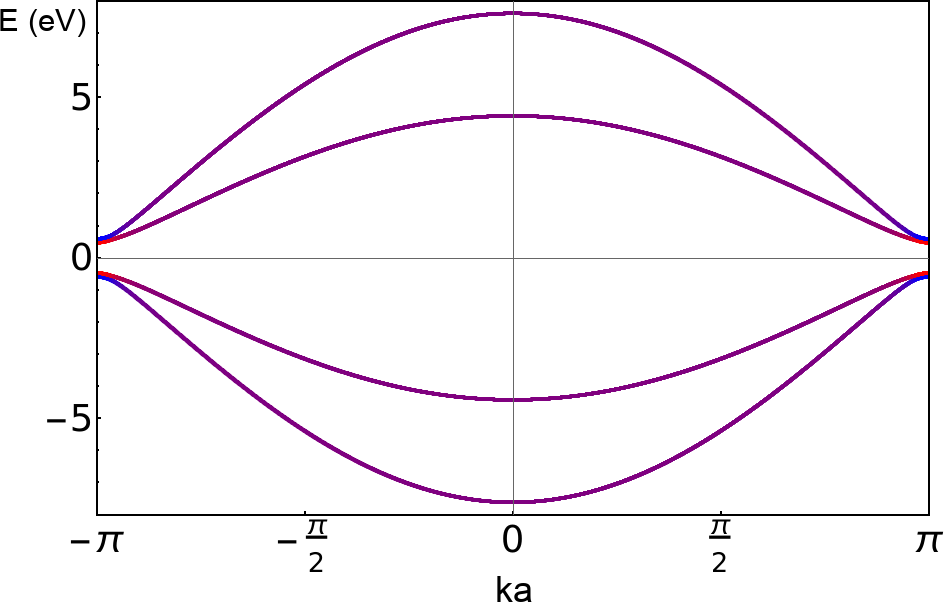
Figure 1: Mean-field energy bands of the two-orbital Hubbard model versus $ka$ for $t_{s0}=t_{d0}=3$, $g_{s}=g_{d}=10$, $\Delta_{s}=\Delta_{d}=0.5$, $\xi a=0.0080$, $t_{sd}=0.8$, and $U=2.0$ (all in eV). The strongly hybridized bands are colored according to their orbital character (blue = $s$, red = $d$, purple = hybridized).

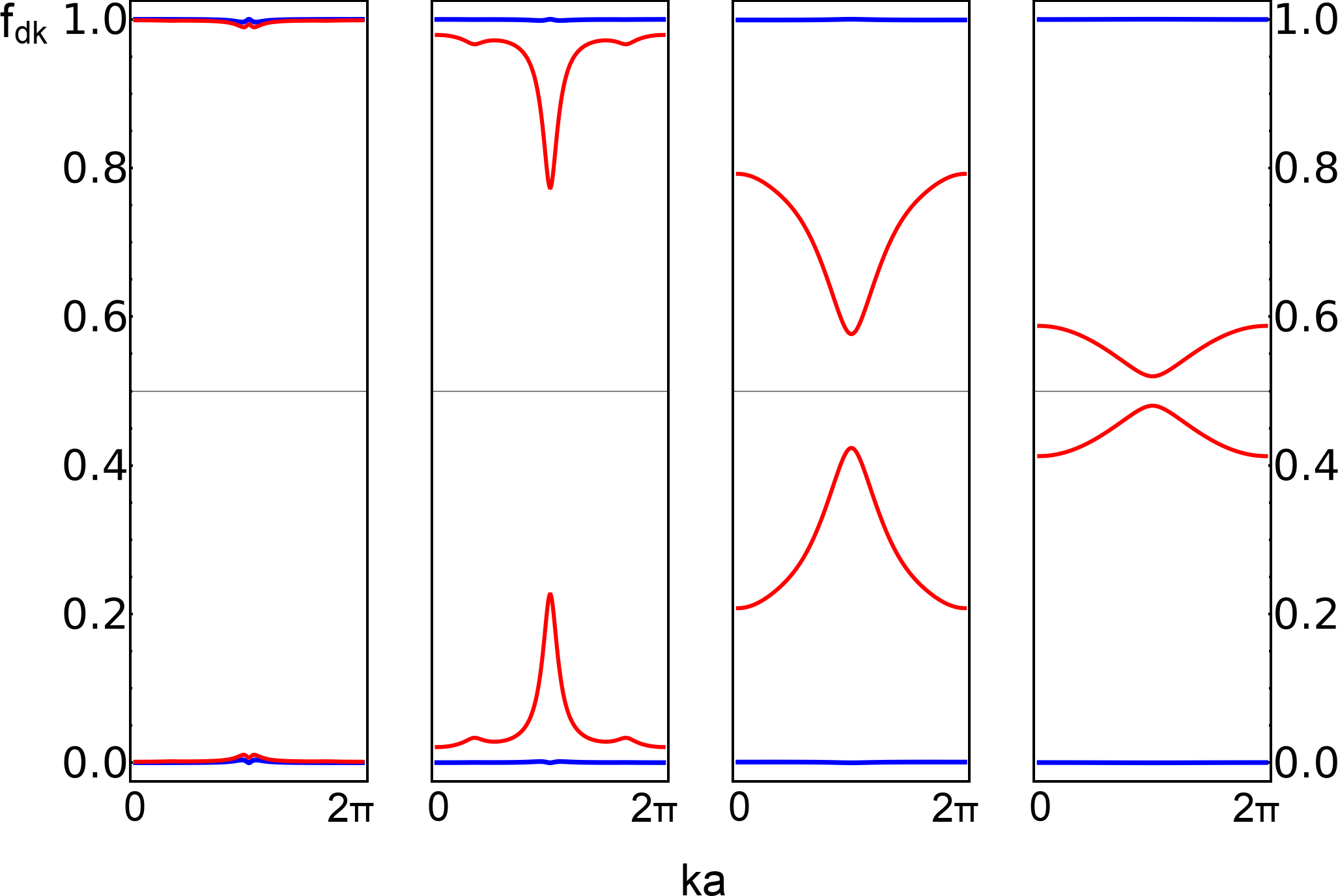
Figure 2: Natural occupation number bands of the two-orbital Hubbard model are shown for the series $U/t_{d0}=0.5,2,8,32$ (left to right) for $t_{s0}=t_{d0}=3$, $g_{s}=g_{d}=10$, $\Delta_{s}=\Delta_{d}=0.5$, $\xi a=0.0080$ and $t_{sd}=0.8$ (all in eV). The predominantly $s$-orbital bands (blue) are close to 0 or 1 for all $U$, while the predominantly $d$-orbital bands (red) split off as $U$ increases. The bands are shown on the domain $ka\in(0,2\pi)$ so that zone boundary is positioned at the center.

Indeed, since the occupation numbers of the weakly correlated bands are very close to 0 and 1, the many-body wavefunction approximately factors into the product of a Slater determinant of weakly correlated orbitals and a strongly correlated wavefunction in the $\mathcal{D}$ subspace, suggesting that a semilocal DFT approximation will provide a sufficiently accurate approximation for the weakly correlated bands. Smooth and continuous natural occupation number bands and natural Bloch orbitals in the true Brillouin zone of the crystal are defined, as described in Ref. Requist and Gross, 2018, by unfolding the bands obtained from the full many-body wavefunction under twisted boundary conditions Thouless (1983); Niu and Thouless (1984) or, equivalently, artificial magnetic fields Kohn (1964).

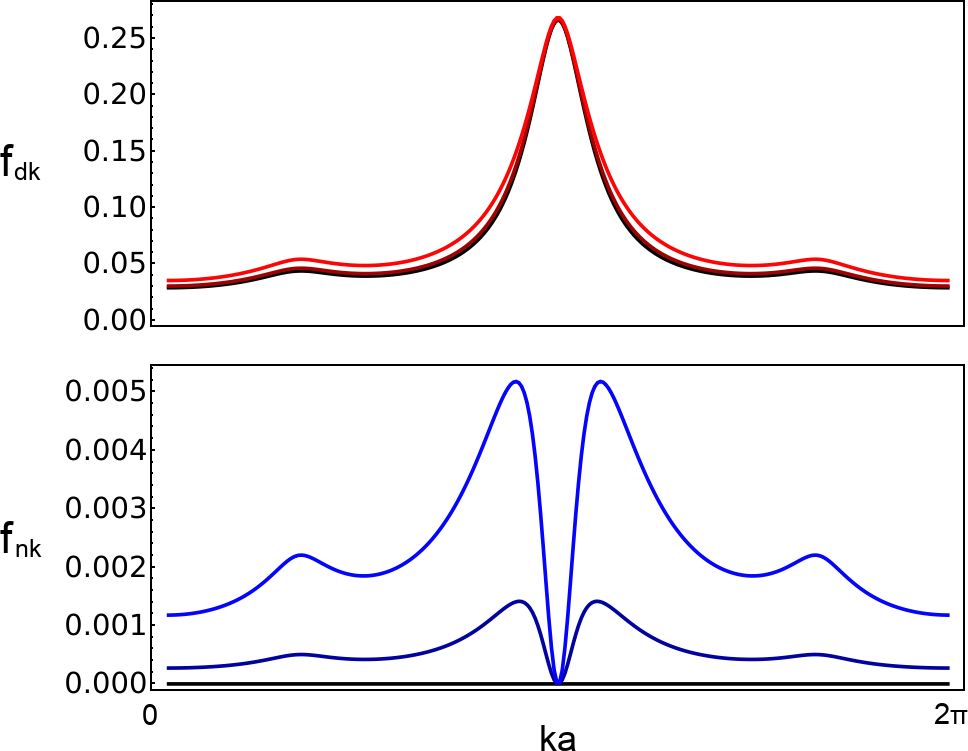
Figure 3: Lower natural occupation number bands of the two-orbital Hubbard model are shown for the series $t_{sd}=0,0.8,1.6$ (dark to light) for $t_{s0}=t_{d0}=3$, $g_{s}=g_{d}=10$, $\Delta_{s}=\Delta_{d}=0.5$, $\xi a=0.0080$ and $U/t_{d0}=2.4$; all parameters in eV.

If we express the Hubbard interactions in Eq. (29) in the basis of the $s$-$d$ hybridized eigenstates of the noninteracting part of $\hat{H}$, we generate Hubbard interactions between $s$-type natural Bloch orbitals as well as interorbital interactions between $s$-type and $d$-type natural Bloch orbitals. Therefore, the $s$-type natural occupation number bands begin to feel the interactions and begin to correlate when the hybridization $t_{sd}$ is turned on. Figure 3 shows that the natural occupation numbers of the $s$ bands correspondingly deviate from 0 and 1 and that this effect increases with increasing $t_{sd}$. However, these deviations still remain much smaller than those of the $d$ bands even for $t_{sd}$ as large as 1.6, and hence we still have a clear separation between weakly and strongly correlated occupation number bands.

V Effective model Hamiltonian

A model Hamiltonian whose minimum yields the occupation numbers $f_{dk}$ and two-body reduced density matrix $\rho_{2}^{d}$ in the strongly correlated subspace was introduced in Sec. II. $f_{dk}$ and $\rho_{2}^{d}$ generally contain contributions from many-body states with all possible occupations of the $d$ bands. As a consequence of the particle-hole symmetry of the two-orbital Hubbard model, the natural occupation number bands have reflection symmetry about $1/2$, i.e. for each $f_{dk}\leq 1/2$, there is another related band with occupation number $1-f_{dk}$ Requist and Gross (2018). Hence, for our chosen supercell, the mean number of electrons occupying the strongly correlated subspace is an integer, $N_{d}=6$. Moreover, in the large $U$ regime, interband fluctuations are suppressed, so that states with $N_{d}\neq 6$ occur with low probability. Therefore, we will attempt to find the model Hamiltonian $\hat{H}^{model,N_{d}}$ with a $6$-electron ground state $|\Phi_{0}^{N_{d}}\rangle$ that contracts to $f_{dk}$ and $\rho_{2}^{d}$.

To make the numerical calculation of the full $|\Psi_{0}\rangle$ manageable, we solve the problem in a restricted but relevant Hilbert space spanned by the sectors with $N_{d}=5$, 6, and 7. More precisely, we include the following three types of states: (a) $N_{d}=6$ states $|\Psi_{a}\rangle=|S_{0}\rangle\otimes|D_{600}\rangle$, (b) $N_{d}=5$ states $|\Psi_{b}\rangle=a_{u,-k,-\sigma}^{{\dagger}}|S_{0}\rangle\otimes|D_{5k\sigma}\rangle$ and (c) $N_{d}=7$ states $|\Psi_{c}\rangle=a_{v,k,\sigma}|S_{0}\rangle\otimes|D_{7k\sigma}\rangle$, where $|D_{N_{d}K_{d}S_{zd}}\rangle$ denotes an $N_{d}$-electron state with total quasimomentum and spin quantum numbers $K_{d}$ and $S_{zd}$, $|S_{0}\rangle=\prod_{vk\sigma}a_{vk\sigma}^{{\dagger}}|0\rangle$ is the six-electron Fermi sea of $s$ electrons; $a_{v,k,\sigma}$ and $a_{u,k,\sigma}^{{\dagger}}$ are the annihilation and creation operators for valence ($v$) and conduction ($u$) band $s$-electron Bloch states. In other words, we only allow a single particle- or hole-type excitation with respect to the reference states of type (a). This is a good approximation in all of our calculations because $U$ is large and $t_{sd}$ is relatively small.

As another consequence of particle-hole symmetry, the only two independent density variables are $n_{s}=\frac{1}{2}(n_{Bs}-n_{As})$ and $n_{d}=\frac{1}{2}(n_{Bd}-n_{Ad})$. In particular, this means that if we write $\hat{H}^{\mathit{model}}$ in the natural orbital basis as

$$\hat{H}^{model} =\sum_{12}\epsilon_{12}c_{d_{1}k_{1}\sigma_{1}}^{{\dagger}}c_{d_{2}k_{2}\sigma_{2}}$$

$$+\sum_{1234}U_{1234}c_{d_{1}k_{1}\sigma_{1}}^{{\dagger}}c_{d_{2}k_{2}\sigma_{2}}^{{\dagger}}c_{d_{4}k_{4}\sigma_{4}}c_{d_{3}k_{3}\sigma_{3}}{,}$$ (34)

then all of the Hamiltonian parameters are functions of $n_{s}$ and $n_{d}$. Here, $c_{dk\sigma}^{{\dagger}}$ is the creation operator for an electron in the natural Bloch orbital state $\phi_{dk\sigma}$ and $1=(d_{1}k_{1}\sigma_{1})$. A quite general approximate form for the two-body model parameters is

$$U_{1234} =\iint\phi_{1}^{*}(\mathbf{r})\phi_{2}^{*}(\mathbf{r}^{\prime})\frac{g_{1234}([n],\mathbf{r},\mathbf{r}^{\prime})}{\epsilon_{0}|\mathbf{r}-\mathbf{r}^{\prime}|}\phi_{3}(\mathbf{r})\phi_{4}(\mathbf{r}^{\prime})d\mathbf{r}d\mathbf{r}^{\prime}{,}$$ (35)

where “screening” is described by the density-dependent factor $g_{1234}([n],\mathbf{r},\mathbf{r}^{\prime})$ and by the self-consistent optimization of the orbitals $\phi_{d\mathbf{k}\sigma}(\mathbf{r})$.

Alternatively, we can also express Eq. (34) in the basis of unique natural Wannier functions Requist and Gross (2018) as

$$\hat{H}^{\mathit{lattice}} =-\sum_{ij,ab}\sum_{\sigma}t_{ij}^{ab}c_{ia\sigma}^{{\dagger}}c_{jb\sigma}$$

$$\quad+\sum_{ijkl,abcd}\sum_{\sigma\tau}U_{ijkl}^{abcd,\sigma\tau}c_{ia\sigma}^{{\dagger}}c_{jb\tau}^{{\dagger}}c_{ld\tau}c_{kc\sigma}+\cdots$$ (36)

where $c_{ia\sigma}^{{\dagger}}$ creates an electron in the natural Wannier state $w_{ia}(\mathbf{r})$ of orbital $a$ at site $i$.

V.1 Practical downfolding scheme

After finding the ground state $|\Psi_{0}\rangle$ of the two-orbital Hubbard model and the density matrix $\hat{\rho}=|\Psi_{0}\rangle\langle\Psi_{0}|$, we use the Löwdin partitioning technique Löwdin (1962) as an efficient means of inferring the model Hamiltonian. Define $\hat{P}$ to be the projector on $12$-electron states that consist of a fully occupied valence $s$ band (six electrons) and all possible $N_{d}=6$ states. The number of such states with total quasimomentum $K=0$ and spin quantum number $S_{z}=0$ is 136. Define $\hat{Q}$ to be the projector onto the orthogonal complement, comprising the sectors with $N_{d}=5$ and $N_{d}=7$. The space spanned by $\hat{Q}$ has a total of $1200$ states with $K=0$ and $S_{z}=0$. The effective Hamiltonian in the $\hat{P}$ sector is

$$\hat{H}^{\mathit{eff}}=\hat{P}\hat{H}\hat{P}+\hat{P}\hat{H}\hat{Q}(E-\hat{Q}\hat{H}\hat{Q})^{-1}\hat{Q}\hat{H}\hat{P}{.}$$ (37)

This Hamiltonian is still exact. Since it depends nonlinearly on $E$, it is not limited to the ground state and has a self-consistent solution for each eigenvalue $E_{n}$. For the purpose of obtaining the most important frequency-independent model parameters of a Hamiltonian $\hat{H}^{model,N_{d}}$ whose ground state is $|\Phi_{0}^{N_{d}}\rangle$, one can substitute $E=E_{0}$ in $\hat{H}^{\mathit{eff}}$ and perform a fitting as described in the next section.

V.2 Density dependence of the model parameters

The model Hamiltonian obtained from Eq. (37) is an a priori unstructured 136$\times$136 matrix on the $N_{d}$-electron Hilbert space with $K=0$ and $S_{z}=0$. For practical calculations, we need to identify a few relevant model parameters to approximate by density functionals. To do so, we first write a trial Hamiltonian in the original site basis

$$\hat{H}^{model} =-t_{d1}^{model}\sum_{i=1}^{3}\sum_{\sigma}(d_{2i-1\sigma}^{{\dagger}}d_{2i\sigma}+H.c.)$$

$$\quad-t_{d2}^{model}\sum_{i=1}^{3}\sum_{\sigma}(d_{2i\sigma}^{{\dagger}}d_{2i+1\sigma}+H.c.)$$

$$\quad+\Delta_{d}^{model}\sum_{i=1}^{3}\sum_{\sigma}(\hat{n}_{2i-1\sigma}-\hat{n}_{2i\sigma})$$

$$\quad+U^{model}\sum_{i=1}^{6}\hat{n}_{i\uparrow}\hat{n}_{i\downarrow}{.}$$ (38)

To determine the model parameters, we perform a least squares minimization of $||\hat{H}^{model}-\hat{H}^{\mathit{eff}}||$ in the Frobenius norm. Then we verify that the ground state of $\hat{H}^{model}$ is close to the ground state of $\hat{H}^{\mathit{eff}}$. In all the calculations we report, $1-|\langle\Phi^{model,N_{d}}_{0}|\Phi^{\mathit{eff},N_{d}}_{0}\rangle|\lesssim 5\times 10^{-4}$. Varying $\Delta_{s}$ and $\Delta_{d}$ in the original Hamiltonian allows us to change $n_{s}$ and $n_{d}$ over a range of values and study the resulting trends in the model parameters. Figure 4 shows the one-to-one relationship between $\Delta_{s}$ and $n_{s}$. Figure 5 shows how the model parameters vary as functions of $\Delta_{s}$. By inverting the $\Delta_{s}\rightarrow n_{s}$ mapping in Fig. 4, we can infer the density dependence of the model parameters. The $n_{s}$-dependence of $t_{d1}^{model}$ and $t_{d2}^{model}$ is negligible for $t_{sd}\lesssim 1$ eV and relatively weak in all cases considered.

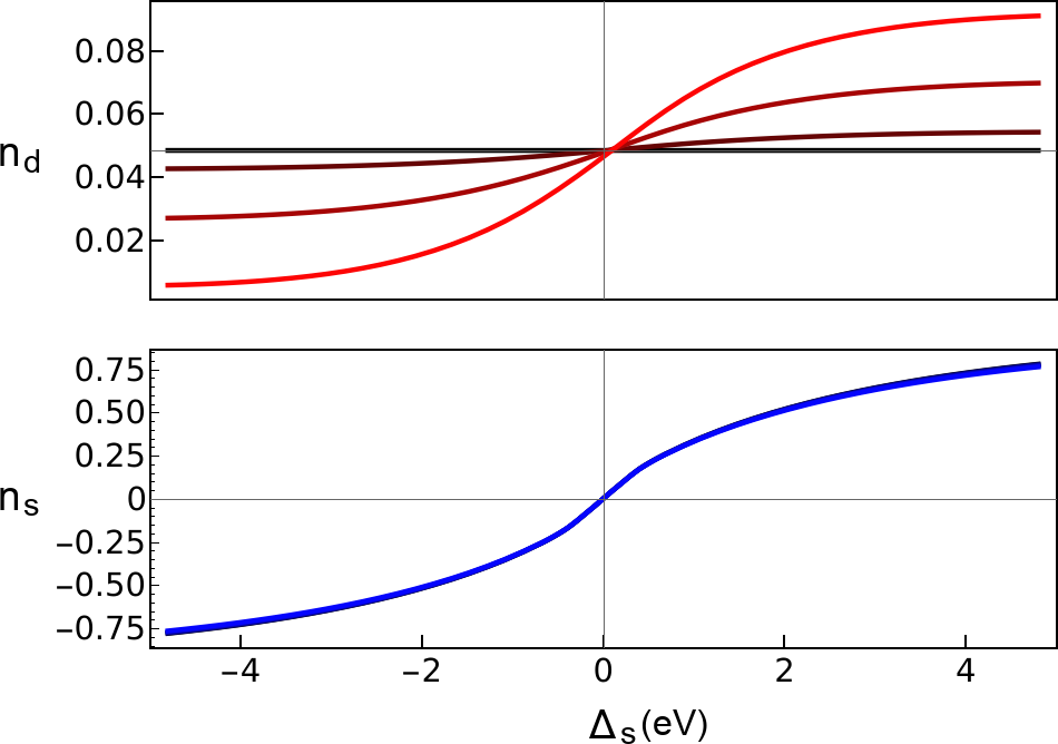
Figure 4: The densities $n_{d}$ (red) and $n_{s}$ (blue) are plotted versus $\Delta_{s}$ for $t_{s0}=t_{d0}=3$, $g_{s}=g_{d}=10$, $\xi a=0.0020$, $\Delta_{d}=0.5$, $U/t_{d0}=2.4$ and for the series $t_{sd}=0.0,0.8,1.6,2.4$ (dark to light); all parameters in eV.

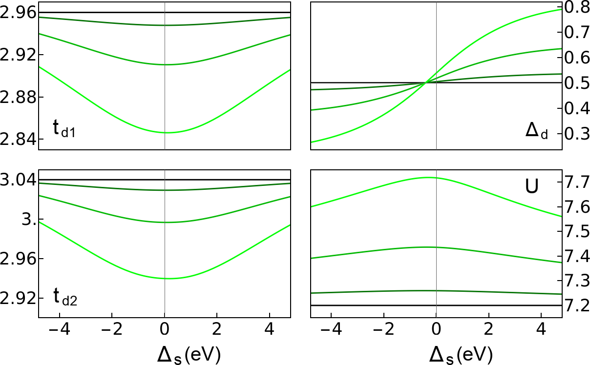
Figure 5: Model parameters $t_{d1}^{model}$ (top left), $t_{d2}^{model}$ (bottom left), $\Delta_{d}^{model}$ (top right) and $U^{model}$ (bottom right) are plotted versus $\Delta_{s}$ for the series $t_{sd}=0.0,0.8,1.6,2.4$ (dark to light) for the same parameters as Fig. 4.

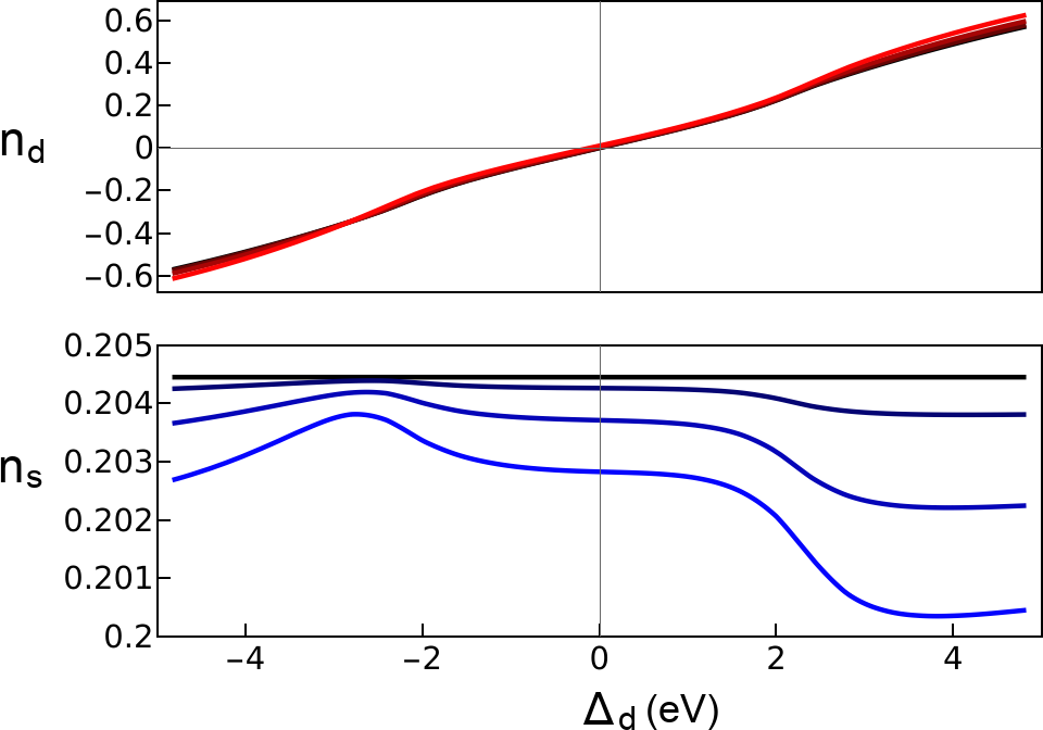
Figure 6: The densities $n_{d}$ (red) and $n_{s}$ (blue) are plotted versus $\Delta_{d}$ for $t_{s0}=t_{d0}=3$, $g_{s}=g_{d}=10$, $\xi a=0.0020$, $\Delta_{s}=0.5$, $U/t_{d0}=2.4$ and for the series $t_{sd}=0.0,0.8,1.6,2.4$ (dark to light); all parameters in eV.

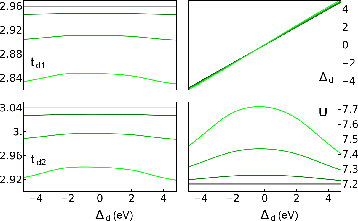
Figure 7: Model parameters $t_{d1}^{model}$ (top left), $t_{d2}^{model}$ (bottom left), $\Delta_{d}^{model}$ (top right) and $U^{model}$ (bottom right) are plotted versus $\Delta_{d}$ for the series $t_{sd}=0.0,0.8,1.6,2.4$ (dark to light) and the same parameters as Fig. 6.

We emphasize that $t_{d1}^{model}$ and $t_{d2}^{model}$ change very little even though $\Delta_{s}$ spans a very large range in Figs. 4 and 5. $\Delta_{d}^{model}$ and $U^{model}$ have moderate but still quite regular $n_{s}$-dependence. Figures 6 and 7 show the dependence of $n_{s}$, $n_{d}$ and the model parameters on $\Delta_{d}$. Here, the trends in $t_{d1}^{model}$, $t_{d2}^{model}$ and $U^{model}$ are similar to those obtained from varying $\Delta_{s}$. On the other hand, $\Delta_{d}^{model}$ has an approximately linear relationship with $\Delta_{d}$, which is expected. These results provide encouraging evidence that simple functional approximations can be found for a model Hamiltonian that describes a few select strongly correlated bands in real materials.

We have considered more general trial Hamiltonians with next-nearest neighbor hopping amplitudes $t_{3}$ and $t_{4}$ and next-next-nearest neighbor hopping $t_{5}$, as well as several different types of two-body interactions. As all of these additional terms are generically nonzero, we observe that the coupling of the $d$ bands to the $s$ bands generates interactions beyond the Hubbard interactions in the original Hamiltonian. However, throughout the range of parameters reported here, these additional terms are small and the Hamiltonian in Eq. (38) is sufficient.

VI Macroscopic polarization

Having obtained a model Hamiltonian whose ground state gives a good approximation to the state of the strongly correlated subspace, we now test how well such a model Hamiltonian and ground state can reproduce the strongly correlated part of the macroscopic polarization. The Ortiz-Martin formula $P=-(e/2\pi)\lim_{N\rightarrow\infty}\gamma(N)$ relates the macroscopic polarization (modulo the polarization quantum) to the many-body geometric phase

$$\gamma(N)=\int_{0}^{2\pi}i\langle\Psi_{0}|\partial_{\alpha}\Psi_{0}\rangle d\alpha{,}$$ (39)

where in our case $|\Psi_{0}(\alpha)\rangle$ is the $12$-electron ground state of the twisted version of the Hamiltonian in Eq. (28) Ortiz and Martin (1994). The twisted Hamiltonian is obtained from $\hat{H}$ by making the Peierls’s substitutions $t_{aj}\rightarrow t_{aj}e^{i\alpha/6}$ (with $a=s,d$ and $j=1,2$) and $t_{sd}\rightarrow t_{sd}e^{i\alpha/6}$.

To evaluate Eq. (39), we express the wavefunction as

$$|\Psi_{0}\rangle=\sum_{D}c_{D}|S(D)\rangle|D\rangle{,}$$ (40)

where $D=(d_{1}k_{1}\sigma_{1},d_{2}k_{2}\sigma_{2},\ldots)$ is a multi-index labeling the strongly correlated $d$-orbital part of the many-body state. The wavefunction in Eq. (40) has a restricted form because we have solved the problem on the restricted Hilbert space consisting of the $N_{d}=$ 5, 6, and 7 sectors defined in Sec. V. Hence, the $s$-electron factor, denoted as $|S(D)\rangle$, is uniquely determined by $|D\rangle$. For example, for a state $|D\rangle$ with $N_{d}=7$, $K_{d}=k$ and $S_{zd}=\sigma$, conservation of particle number, quasimomentum and $z$-projection of spin imply $|S(D)\rangle=a_{vk\sigma}|S_{0}\rangle$. Thus, for our system, the geometric phase in Eq. (39) is

$$\gamma =\sum_{D}\int_{0}^{2\pi}ic_{D}^{*}\partial_{\alpha}c_{D}d\alpha$$

$$+\sum_{N_{d}K_{d}S_{zd}}\int_{0}^{2\pi}iP_{N_{d}K_{d}S_{zd}}\sum_{nk\sigma}f_{nk\sigma}^{N_{d}K_{d}S_{zd}}\langle\phi_{nk\sigma}|\partial_{\alpha}\phi_{nk\sigma}\rangle d\alpha{,}$$ (41)

where $P_{N_{d}K_{d}S_{zd}}(\alpha)=\sum_{D}^{(N_{d}K_{d}S_{zd})}|c_{D}(\alpha)|^{2}$ and $f_{nk\sigma}^{N_{d}K_{d}S_{zd}}$ is the occupation number (0 or 1) of the $s$-orbital $\phi_{nk\sigma}$ in the Slater determinant $|S(D_{N_{d}K_{d}S_{zd}})\rangle$. After unfolding the natural occupation numbers and natural Bloch orbitals to the full Brillouin zone Requist and Gross (2018), the geometric phase simplifies to

$$\gamma =\int_{0}^{2\pi}i\langle\Phi_{0}^{N_{d}}|\partial_{\alpha}\Phi_{0}^{N_{d}}\rangle d\alpha$$

$$\quad+\sum_{\sigma,n\in\mathcal{S}}\int_{0}^{2\pi/a}if_{nk\sigma}\langle\tilde{u}_{nk\sigma}|\partial_{k}\tilde{u}_{nk\sigma}\rangle dk{.}$$ (42)

The first term has been expressed in terms of the ground state $|\Phi_{0}^{N_{d}}\rangle$ of the twisted model Hamiltonian, while the second term is given in terms of the periodic part $\tilde{u}_{nk\sigma}$ of the $s$-electron Bloch orbital $\phi_{nk\sigma}$. Given that the occupation numbers $f_{nk\sigma}=\sum_{N_{d}K_{d}S_{zd}}P_{N_{d}K_{d}S_{zd}}f_{nk\sigma}^{N_{d}K_{d}S_{zd}}$ of the $s$-electron Bloch orbitals are close to $0$ or $1$, we suppose that the second term can be well-approximated by the geometric phase of noninteracting electrons as in the King-Smith–Vanderbilt formula, i.e.

$$\gamma_{s}^{KS}=\sum_{n\sigma}\int_{0}^{2\pi/a}ig_{nk\sigma}\langle u_{nk\sigma}|\partial_{k}u_{nk\sigma}\rangle dk{,}$$ (43)

where the occupation numbers $g_{nk\sigma}$ (0 or 1) restrict the sum to the occupied $s$-electron Kohn-Sham-like states $\chi_{nk\sigma}(r)=e^{ikr}u_{nk\sigma}(r)$. Although we expect Eq. (43) to be an accurate approximation for the weakly correlated bands in line with the successful application of the King-Smith–Vanderbilt formula to weakly correlated systems, the polarization calculated by Eq. (42) with the approximation in Eq. (43) is not exact. It might be possible to extend our theory to an exact theory for the macroscopic polarization by including additional basic variables in analogy to the inclusion of the polarization in standard DFT Gonze et al. (1995, 1997); Martin and Ortiz (1997).

We begin by presenting results for the exact geometric phase calculated with Eq. (42). The first term of Eq. (42), which we denote as $\gamma_{d}$, is the contribution of the strongly correlated $d$-electron wavefunction. Since $\gamma_{d}$ has equal contributions from spin up and spin down electrons, we define $\gamma_{d\sigma}=\gamma_{d}/2$. The second term, $\gamma_{s}$, is the contribution of the weakly correlated $s$-electron bands, and we further define $\gamma_{s\sigma}=\gamma_{s}/2$. $\gamma_{d\sigma}$ and $\gamma_{s\sigma}$ are shown versus $\Delta_{d}$ in Fig. 8. As the $s$ electrons only feel the bias indirectly through their hybridization with the $d$ bands, $\gamma_{s\sigma}$ has a weak dependence on $\Delta_{d}$. On the other hand, $\gamma_{d\sigma}$ has a nontrivial dependence on $\Delta_{d}$. The plateau between $\Delta_{d}=-2$ and 2 eV is due to Hubbard interactions; $\Delta_{d}$ can only polarize the $d$-electron states if it can overcome the on-site repulsion $U$. The effects of correlations on $\gamma_{d\sigma}$ are evident upon comparison with the geometric phase of the noninteracting version ($U=0$) of the two-orbital Hubbard model, which is shown in Fig. 9.

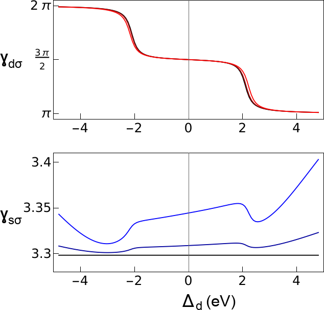
Figure 8: Many-body geometric phases $\gamma_{d\sigma}$ (red) and $\gamma_{s\sigma}$ (blue) for the two-orbital Hubbard model are plotted versus $\Delta_{d}$ for the series $t_{sd}=0,0.8,1.6$ eV (dark to light) and the same parameters as Fig. 6.

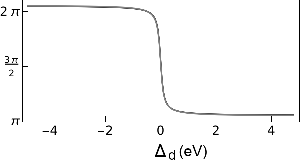
Figure 9: Geometric phase $\gamma_{d\sigma}+(\gamma_{s\sigma}-\pi)$ for the noninteracting two-orbital Hubbard model is plotted versus $\Delta_{d}$ for the series $t_{sd}=0,0.8,1.6$ (dark to light gray) and the same parameters as Fig. 8. The curves for different values of $t_{sd}$ nearly coincide.

So far we have presented results for the exact $|\Psi_{0}(\alpha)\rangle$. Now we ask how well the ground state $|\Phi_{0}^{model,N_{d}}\rangle$ of the fitted model Hamiltonian reproduces $\gamma_{d\sigma}$. In principle, the model Hamiltonian parameters will be $\alpha$-dependent. However, we can make the following approximation. We assume that the moduli of the hopping parameters $t_{d1}^{model}$ and $t_{d2}^{model}$ are approximately constant but that their phases vary as functions of $\alpha$ exactly as the bare hopping parameters do under the Peierls’s substitution. Under this approximation, the only information we need to evaluate $\gamma_{d\sigma}$ are the parameters of the untwisted model Hamiltonian ($\alpha=0$). To test the validity of this approximation, we use the $\alpha=0$ model parameters from Fig. 7 to calculate $\gamma_{d,\mathit{approx}}$ (dashed green) and compare it with the exact result (black) in Fig. 10. The results are shown together with the mean-field (Hartree-Fock) approximation. First, they demonstrate that the ground state of $\hat{H}^{model}(\alpha)$, obtained by performing the Peierls’s substitution to $\hat{H}^{model}(0)$, yields an accurate approximation to the strongly correlated part of the full geometric phase. Second, they reveal that the paramagnetic mean-field approximation (gray) fails qualitatively. The broken-symmetry antiferromagnetic mean-field approximation (orange) improves the behavior for small $\Delta_{d}$ but fails for $1.75\lesssim\Delta_{d}\lesssim 3.5$ eV. Semilocal (spin-)DFT approximations will give comparably incorrect results.

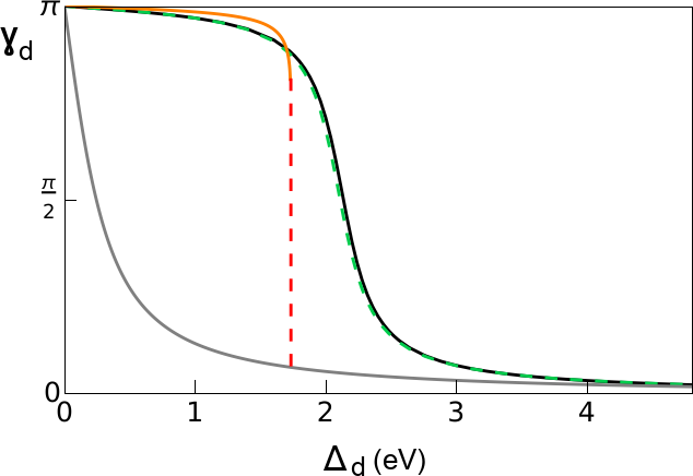
Figure 10: Comparison of $\gamma_{d}$ from the full solution of the two-orbital Hubbard model (black), the model Hamiltonian solution (dashed green) and mean-field approximations (orange and gray) for $t_{s0}=3$, $t_{d0}=3$, $\xi=0.0020$, $\Delta_{s}=0.5$, $U/t_{d0}=2.4$ and $t_{sd}=0.8$ as functions of $\Delta_{d}$; all parameters in eV. The dashed red line connects the paramagnetic (gray) and antiferromagnetic (orange) mean-field results.

Bethe Ansatz local density approximation (BALDA) Lima et al. (2003); Schönhammer et al. (1995) uses the one-dimensional Hubbard model as a reference system from which to derive the exchange-correlation energy density as a function of the average site occupation. The BALDA exchange-correlation energy density can be used to calculate the density of inhomogeneous lattice models such as Hubbard models with staggered potentials. Since, by construction, the BALDA yields the exact energy and density for a uniform one-dimensional lattice model for any $U$, one might expect it to be capable of reproducing the strongly correlated part of the geometric phase. To test this, we have evaluated the geometric phase $\gamma_{d,\mathit{BALDA}}$ of the Rice-Mele-Hubbard model by substituting the BALDA Kohn-Sham eigenstates into the King-Smith–Vanderbilt formula. As shown in Fig. 11, $\gamma_{d,\mathit{BALDA}}$ agrees with the exact geometric phase for $U=0$ but is qualitatively incorrect for moderate and large $U$. We conclude that functional approximations that yield good densities do not necessarily yield accurate values for the geometric phase, which depends on how the $\mathbf{k}$-dependent phases of the Bloch functions vary across the Brillouin zone.

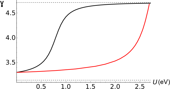
Figure 11: Comparison of BALDA (red) and exact (black) results for the geometric phase in the Rice-Mele-Hubbard as a function of $U$ for $t_{d0}=3$, $g_{d}=10$, $\Delta_{d}=0.5$ and $\xi=0.0020$; all parameters in eV. Dashed lines show $\pi$ and $3\pi/2$.

VII Conclusions

Self-consistently coupling density functional theory to a model Hamiltonian (“DFT+model”) was shown to yield accurate results for the macroscopic polarization in a strongly correlated system where all known DFT approximations fail qualitatively. DFT+model is an efficient ab initio framework for calculating geometric and topological invariants in strongly correlated materials. The application of the theory to the calculation of topological invariants is a problem for future work. The fact that the theory reliably reproduces the macroscopic polarization — a geometric quantity closely related to topological invariants — over a wide range of parameters, as we have observed here, is strong evidence that it will also give accurate results for topological invariants.

The theory establishes a systematic and self-consistent ab initio procedure for constructing the unique model Hamiltonian for the subset of strongly correlated degrees of freedom. This is the only model Hamiltonian that yields the correct equilibrium occupation numbers $f_{d\mathbf{k}}$ and two-body reduced density matrix $\rho_{2}^{d}$ in the strongly correlated subspace. The two-body reduced density matrix $\rho_{2}^{d}$ contains the information about all two-body correlation functions. The model Hamiltonian does not depend on a separation of energy scales or the existence of a set of narrow mean-field energy bands. Identifying the strongly correlated orbitals from the natural occupation number band structure is a novel way of singling out strongly correlated degrees of freedom in solids.

As opposed to $GW$+DMFT Biermann et al. (2003); Sun and Kotliar (2004); Tomczak et al. (2012); Ayral et al. (2012); Hansmann et al. (2013); Tomczak et al. (2014); Biermann (2014) and other DMFT-based methods, our theory does not involve any frequency dependence. This does not imply any approximation but entails certain advantages and disadvantages. One advantage is the greater efficiency of the many-body part of our self-consistency cycle, which involves solving for the equilibrium state of a many-body Hamiltonian rather than solving a self-consistent impurity problem with frequency-dependent interactions, e.g. $U(\omega)$, as in some DMFT implementations Werner and Millis (2010). On the other hand, the lack of frequency dependence might make it more difficult to obtain spectral functions in our theory. It would be interesting to explore how well the excitations of the model Hamiltonian represent the true strongly correlated excitations of the system, although we emphasize that our model Hamiltonian is only guaranteed to reproduce the equilibrium occupations and two-body correlations and not any other observables. Another important distinction with DMFT-based approaches is the fact that our theory preserves the full crystal symmetry of the original Hamiltonian including $\mathbf{k}$-dependent correlations, which are neglected in conventional DMFT. The $\mathbf{k}$-dependence is crucial for properly evaluating geometric and topological quantities in strongly correlated materials. Symmetry constraints on the structure of the $\mathbf{k}$-dependent correlations may enable improved accuracy. Recent extensions of DMFT aim to incorporate nonlocal correlations Lechermann et al. (2017).

Adapting the present theory to finite systems in which the strongly correlated subspace is taken to be spanned by just a few natural orbitals Requist and Pankratov (2011), such as localized orbitals in Kondo systems or hybridized transition metal orbitals in molecules, would constitute a novel embedding theory that might allow one to obtain more accurate ab initio results for systems with strong static correlation and partially circumvent the problem of memory dependence in TDDFT. This would be especially helpful in the modeling of coupled electron-ion dynamics within exact factorization density functional theory Requist and Gross (2016); Li et al. (2018).

Appendix A Generalized Kohn-Sham scheme

The role of the on-site $d$-orbital density matrix and orbital-dependent potentials in the DFT+$U$ method Anisimov et al. (1991); Liechtenstein et al. (1995); Anisimov et al. (1997a); Pickett et al. (1998); Cococcioni and de Gironcoli (2005); Nakamura et al. (2006); Himmetoglu et al. (2013), as well as the uncertainties arising from the strongly correlated narrow Fe bands in semilocal DFT calculations of the pressure-induced spin state crossover in Fe_xMg_1-xSiO₃ perovskite Umemoto et al. (2008), motivated the investigation of an effective single-particle Hamiltonian for a strongly correlated Hubbard model in a reduced density matrix approach Requist and Pankratov (2008). As in the DFT+$U$ method, it was assumed that the nonlocal, orbital-dependent part of the effective potential would only be applied to a subset of strongly correlated degrees of freedom. In this Appendix, we show that the part of the nonlocal effective potential acting in the strongly correlated subspace can be rigorously combined with a multiplicative Kohn-Sham potential to define a generalized Kohn-Sham Hamiltonian.

For fixed $(f_{d\mathbf{k}},\rho_{2}^{d})$, the density, paramagnetic current density, and strongly correlated natural Bloch orbitals can be obtained by self-consistently solving a generalized Kohn-Sham equation. We start by defining the following grand potential functional for a system of noninteracting electrons in the presence of local scalar and vector potentials $v_{s}(\mathbf{r})$ and $\mathbf{A}_{s}(\mathbf{r})$ and a nonlocal potential $w(\mathbf{r}\sigma,\mathbf{r}^{\prime}\sigma^{\prime})=\sum_{d\mathbf{k}d^{\prime}\mathbf{k}^{\prime}}w_{d\mathbf{k},d^{\prime}\mathbf{k}^{\prime}}\phi_{d\mathbf{k}\sigma}(\mathbf{r})\phi_{d^{\prime}\mathbf{k}^{\prime}\sigma^{\prime}}^{*}(\mathbf{r})$:

$$\Omega_{s}[n,\mathbf{j}_{p},\phi_{d\mathbf{k}},f_{d\mathbf{k}}] =K_{s}[n,\mathbf{j}_{p},\phi_{d\mathbf{k}},f_{d\mathbf{k}}]+\frac{e}{c}\int\mathbf{A}_{s}(\mathbf{r})\cdot\mathbf{j}_{p}(\mathbf{r})d\mathbf{r}$$

$$+\int\Big{[}\frac{e^{2}}{2mc^{2}}|\mathbf{A}_{s}(\mathbf{r})|^{2}+v_{s}(\mathbf{r})-\mu\Big{]}n(\mathbf{r})d\mathbf{r}$$

$$+\sum_{\sigma\sigma^{\prime}}\int w(\mathbf{r}\sigma,\mathbf{r}^{\prime}\sigma^{\prime})\rho_{1}(\mathbf{r}^{\prime}\sigma^{\prime},\mathbf{r}\sigma)d\mathbf{r}d\mathbf{r}^{\prime}{.}$$ (44)

The ensemble kinetic-energy-entropy functional is

$$K_{s}[n,\mathbf{j}_{p},\phi_{d\mathbf{k}},f_{d\mathbf{k}}] =\min_{\rho_{s}\rightarrow(n,\mathbf{j}_{p},\phi_{d\mathbf{k}},f_{d\mathbf{k}})}\mathrm{Tr}[(\hat{T}-\tau\hat{S}_{s})\hat{\rho}_{s}]$$

$$=\sum_{n\mathbf{k}\sigma}^{\mathcal{S}}g_{n\mathbf{k}\sigma}\langle\chi_{n\mathbf{k}\sigma}|\hat{T}|\chi_{n\mathbf{k}\sigma}\rangle$$

$$+\sum_{d\mathbf{k}\sigma}^{\mathcal{D}}f_{d\mathbf{k}\sigma}\langle\phi_{d\mathbf{k}\sigma}|\hat{T}|\phi_{d\mathbf{k}\sigma}\rangle$$

$$+k_{B}\tau\sum_{b\mathbf{k}}[f_{b\mathbf{k}}\ln f_{b\mathbf{k}}$$

$$\quad+(1-f_{b\mathbf{k}})\ln(1-f_{b\mathbf{k}})]{,}$$ (45)

where $\hat{T}=-\hbar^{2}\nabla^{2}/2m$ and the sum over $b\mathbf{k}$ runs over both $\mathcal{S}$ and $\mathcal{D}$ with $f_{b\mathbf{k}}=f_{d\mathbf{k}}$ for $b\mathbf{k}\in\mathcal{D}$ and $f_{b\mathbf{k}}=g_{n\mathbf{k}}$ for $b\mathbf{k}\in\mathcal{S}$. The weakly correlated orbitals in $\mathcal{S}$ are denoted $\chi_{n\mathbf{k}}$, the strongly correlated orbitals in $\mathcal{D}$ are denoted $\phi_{d\mathbf{k}}$, and a generic eigenstate from either $\mathcal{S}$ or $\mathcal{D}$ is denoted $\psi_{b\mathbf{k}}$. In Eq. (45), we have allowed for the possibility that the equilibrium state, even at $\tau=0$, is an ensemble state Requist and Pankratov (2008) formed from degenerate Slater determinants $|\Phi_{I}\rangle$ according to

$$\rho_{s}=\sum_{I}w_{I}|\Phi_{I}\rangle\langle\Phi_{I}|{;}\quad\sum_{I}w_{I}=1{.}$$ (46)

The unknown ensemble weights are related to the occupation numbers according to

$$\sum_{I}\Theta_{n\mathbf{k},I}w_{I} =g_{n\mathbf{k}}\quad\mathrm{if}\;n\mathbf{k}\in\mathcal{S}$$

$$\sum_{I}\Theta_{d\mathbf{k},I}w_{I} =f_{d\mathbf{k}}\quad\mathrm{if}\;d\mathbf{k}\in\mathcal{D}{,}$$ (47)

where $\Theta_{b\mathbf{k},I}=1$ if the orbital $\psi_{b\mathbf{k}}$ is an element of the Slater determinant $|\Phi_{I}\rangle$ and $0$ otherwise Dreizler and Gross (1990). Then, we define the functional

$$G_{s}[n,\mathbf{j}_{p},\phi_{d\mathbf{k}},f_{d\mathbf{k}}] =\Omega_{s}[n,\mathbf{j}_{p},\phi_{d\mathbf{k}},f_{d\mathbf{k}}]$$

$$-\sum_{b\mathbf{k}\neq b^{\prime}\mathbf{k}^{\prime}}\lambda_{b\mathbf{k},b^{\prime}\mathbf{k}^{\prime}}^{s}\int\phi_{b^{\prime}\mathbf{k}^{\prime}}^{*}(\mathbf{r})\phi_{b\mathbf{k}}(\mathbf{r})d\mathbf{r}{.}$$ (48)

Taking variations with respect to $\phi_{d\mathbf{k}}(\mathbf{r})$ and $\phi_{d\mathbf{k}}^{*}(\mathbf{r})$ leads to the stationary conditions

$$f_{d\mathbf{k}}\big{<}\phi_{d^{\prime}\mathbf{k}^{\prime}}\big{|}\hat{H}_{s,\mathit{local}}+\hat{W}_{s}\big{|}\phi_{d\mathbf{k}}\big{>} =\lambda_{d^{\prime}\mathbf{k}^{\prime},d\mathbf{k}}^{s}$$

$$f_{d^{\prime}\mathbf{k}^{\prime}}\big{<}\phi_{d^{\prime}\mathbf{k}^{\prime}}\big{|}\hat{H}_{s,\mathit{local}}+\hat{W}_{s}\big{|}\phi_{d\mathbf{k}}\big{>} =\lambda_{d^{\prime}\mathbf{k}^{\prime},d\mathbf{k}}^{s}{,}$$ (49)

where $\hat{H}_{s,\mathit{local}}=-\hbar^{2}\nabla^{2}/2m+(e/c)\int\mathbf{A}_{s}(\mathbf{r})\cdot\hat{\mathbf{j}}_{p}(\mathbf{r})d\mathbf{r}+\int[(e^{2}/2mc^{2})|\mathbf{A}_{s}(\mathbf{r})|^{2}+v_{s}(\mathbf{r})-\mu]\hat{n}(\mathbf{r})d\mathbf{r}$ and $\hat{W}_{s}=\iint\hat{\psi}^{{\dagger}}(\mathbf{r})w(\mathbf{r},\mathbf{r}^{\prime})\hat{\psi}(\mathbf{r}^{\prime})$. By subtraction, we find

$$(f_{d\mathbf{k}}-f_{d^{\prime}\mathbf{k}^{\prime}})\big{<}\phi_{d^{\prime}\mathbf{k}^{\prime}}\big{|}\hat{T}+\hat{V}_{s}+\hat{W}_{s}\big{|}\phi_{d\mathbf{k}}\big{>}=0{.}$$ (50)

Setting $\delta G_{s}/\delta n(\mathbf{r})=0$ and $\delta G_{s}/\delta\mathbf{j}_{p}(\mathbf{r})=0$ gives

$$v_{s}(\mathbf{r})-\mu+\frac{e^{2}}{2mc^{2}}|\mathbf{A}_{s}(\mathbf{r})|^{2}+\left.\frac{\delta K_{s}}{\delta n(\mathbf{r})}\right|_{\phi_{d\mathbf{k}},f_{d\mathbf{k}}} =0$$

$$\frac{e}{c}\mathbf{A}_{s}(\mathbf{r})+\left.\frac{\delta K_{s}}{\delta\mathbf{j}_{p}(\mathbf{r})}\right|_{\phi_{d\mathbf{k}},f_{d\mathbf{k}}} =0{.}$$ (51)

Next, we recall the grand potential functional in Eq. (3) for a system of interacting electrons in the presence of scalar and vector potentials $v(\mathbf{r})$ and $\mathbf{A}(\mathbf{r})$

$$\Omega[n,\mathbf{j}_{p},\phi_{d\mathbf{k}},f_{d\mathbf{k}},\rho_{2}^{d}] =K_{s}[n,\mathbf{j}_{p},\phi_{d\mathbf{k}},f_{d\mathbf{k}}]$$

$$+\frac{e}{c}\int\mathbf{A}(\mathbf{r})\cdot\mathbf{j}_{p}(\mathbf{r})d\mathbf{r}$$

$$+\int\Big{[}\frac{e^{2}}{2mc^{2}}|\mathbf{A}(\mathbf{r})|^{2}+v(\mathbf{r})-\mu\Big{]}n(\mathbf{r})d\mathbf{r}$$

$$+\Omega_{hxc}[n,\mathbf{j}_{p},\phi_{d\mathbf{k}},f_{d\mathbf{k}},\rho_{2}^{d}]$$ (52)

and introduce

$$G[n,\mathbf{j}_{p},\phi_{d\mathbf{k}},f_{d\mathbf{k}},\rho_{2}^{d}] =\Omega[n,\mathbf{j}_{p},\phi_{d\mathbf{k}},f_{d\mathbf{k}},\rho_{2}^{d}]$$

$$-\sum_{d\mathbf{k},d^{\prime}\mathbf{k}^{\prime}}\lambda_{d\mathbf{k},d^{\prime}\mathbf{k}^{\prime}}\int\phi_{d^{\prime}\mathbf{k}^{\prime}}^{*}(\mathbf{r})\phi_{d\mathbf{k}}(\mathbf{r})d\mathbf{r}{.}$$

The stationary conditions for variations of $G$ with respect to $\phi_{d\mathbf{k}}(\mathbf{r})$ and $\phi_{d\mathbf{k}}^{*}(\mathbf{r})$ are

$$f_{d\mathbf{k}}\big{<}\phi_{d^{\prime}\mathbf{k}^{\prime}}\big{|}\hat{H}_{\mathit{local}}\big{|}\phi_{d\mathbf{k}}\big{>} +\left.\bigg{<}\phi_{d^{\prime}\mathbf{k}^{\prime}}\bigg{|}\frac{\delta\Omega_{hxc}}{\delta\phi_{d\mathbf{k}}^{*}}\bigg{>}\right|_{n,\mathbf{j}_{p}}=\lambda_{d^{\prime}\mathbf{k}^{\prime},d\mathbf{k}}$$

$$f_{d^{\prime}\mathbf{k}^{\prime}}\big{<}\phi_{d^{\prime}\mathbf{k}^{\prime}}\big{|}\hat{H}_{\mathit{local}}\big{|}\phi_{d\mathbf{k}}\big{>} +\left.\bigg{<}\frac{\delta\Omega_{hxc}}{\delta\phi_{d^{\prime}\mathbf{k}^{\prime}}}\bigg{|}\phi_{d\mathbf{k}}\bigg{>}\right|_{n,\mathbf{j}_{p}}=\lambda_{d^{\prime}\mathbf{k}^{\prime},d\mathbf{k}}{,}$$ (53)

where $\hat{H}_{\mathit{local}}=-\hbar^{2}\nabla^{2}/2m+(e/c)\int[\mathbf{A}(\mathbf{r})+\mathbf{A}_{xc}(\mathbf{r})]\cdot\hat{\mathbf{j}}_{p}(\mathbf{r})d\mathbf{r}+\int[(e^{2}/2mc^{2})|\mathbf{A}(\mathbf{r})|^{2}+v(\mathbf{r})+v_{hxc}(\mathbf{r})-\mu]\hat{n}(\mathbf{r})d\mathbf{r}$ and, as in current-DFT Vignale and Rasolt (1987), we define

$$v_{hxc}(\mathbf{r}) =\left.\frac{\delta\Omega_{hxc}}{\delta n(\mathbf{r})}\right|_{\phi_{d\mathbf{k}},f_{d\mathbf{k}}}$$

$$\frac{e}{c}\mathbf{A}_{xc}(\mathbf{r}) =\left.\frac{\delta\Omega_{hxc}}{\delta\mathbf{j}_{p}(\mathbf{r})}\right|_{\phi_{d\mathbf{k}},f_{d\mathbf{k}}}{.}$$ (54)

Subtraction leads to

$$(f_{d\mathbf{k}}-f_{d^{\prime}\mathbf{k}^{\prime}})\big{<}\phi_{d^{\prime}\mathbf{k}^{\prime}}\big{|}\hat{T}+\hat{V}\big{|}\phi_{d\mathbf{k}}\big{>}$$

$$+\left.\bigg{<}\phi_{d^{\prime}\mathbf{k}^{\prime}}\bigg{|}\frac{\delta\Omega_{hxc}}{\phi_{d\mathbf{k}}^{*}}\bigg{>}\right|_{n,\mathbf{j}_{p}}-\left.\bigg{<}\frac{\delta\Omega_{hxc}}{\phi_{d^{\prime}\mathbf{k}^{\prime}}}\bigg{|}\phi_{d\mathbf{k}}\bigg{>}\right|_{n,\mathbf{j}_{p}}=0{.}$$ (55)

The variations of $G$ with respect to $n(\mathbf{r})$ and $\mathbf{j}_{p}(\mathbf{r})$ for fixed $(\phi_{d\mathbf{k}},f_{d\mathbf{k}})$ give

$$v(\mathbf{r})+v_{hxc}(\mathbf{r})+\frac{e^{2}}{2mc^{2}}|\mathbf{A}(\mathbf{r})|^{2}-\mu+\left.\frac{\delta K_{s}}{\delta n(\mathbf{r})}\right|_{\phi_{d\mathbf{k}},f_{d\mathbf{k}}} =0$$

$$\frac{e}{c}\mathbf{A}(\mathbf{r})+\frac{e}{c}\mathbf{A}_{xc}(\mathbf{r})+\left.\frac{\delta K_{s}}{\delta\mathbf{j}_{p}(\mathbf{r})}\right|_{\phi_{d\mathbf{k}},f_{d\mathbf{k}}} =0{.}$$ (56)

The stationary conditions in Eqs. (55) and (56) are the same as those of the noninteracting system, Eqs. (50) and (51), if we define

$$v_{s}(\mathbf{r}) =v(\mathbf{r})+v_{hxc}(\mathbf{r})+\frac{e^{2}}{2mc^{2}}\big{(}|\mathbf{A}(\mathbf{r})|^{2}-|\mathbf{A}_{s}(\mathbf{r})|^{2}\big{)}$$

$$\mathbf{A}_{s}(\mathbf{r}) =\mathbf{A}(\mathbf{r})+\mathbf{A}_{xc}(\mathbf{r})$$ (57)

and if we define $\hat{W}_{s}$ by

$$\langle\phi_{d^{\prime}\mathbf{k}^{\prime}}|\hat{W}_{s}|\phi_{d\mathbf{k}}\rangle=\frac{\left.\Big{<}\phi_{d^{\prime}\mathbf{k}^{\prime}}\Big{|}\frac{\delta\Omega_{hxc}}{\delta\phi_{d\mathbf{k}}^{*}}\Big{>}\right|_{n,\mathbf{j}_{p}}-\left.\Big{<}\frac{\delta\Omega_{hxc}}{\delta\phi_{d^{\prime}\mathbf{k}^{\prime}}}\Big{|}\phi_{d\mathbf{k}}\Big{>}\right|_{n,\mathbf{j}_{p}}}{f_{d\mathbf{k}}-f_{d^{\prime}\mathbf{k}^{\prime}}}$$ (58)

for $d\mathbf{k}\neq d^{\prime}\mathbf{k}^{\prime}$. A similar expression for a nonlocal effective potential has been derived Pernal (2005) in the context of reduced density matrix functional theory at $\tau=0$ Gilbert (1975), where the energy is a functional of all natural orbitals and the orbital derivatives are not constrained to fixed $(n,\mathbf{j}_{p})$. We can obtain the equilibrium $n(\mathbf{r})$, $\mathbf{j}_{p}(\mathbf{r})$, and $\phi_{d\mathbf{k}}(\mathbf{r})$ by self-consistently solving a single-particle Schrödinger equation with the Hamiltonian

$$\hat{h}^{\mathit{eff}}=\frac{1}{2m}\big{(}\hat{\mathbf{p}}+\frac{e}{c}\mathbf{A}_{s}(\hat{\mathbf{r}})\big{)}^{2}+\hat{V}_{s}+\hat{W}_{s}{,}$$ (59)

where $\hat{V}_{s}=\int v_{s}(\mathbf{r})\hat{n}(\mathbf{r})d\mathbf{r}$, together with the expressions for $n(\mathbf{r})$ and $\mathbf{j}_{p}(\mathbf{r})$ in Eq. (11). The eigenvalues will obey

$$\begin{array}[]{ll}\epsilon_{n\mathbf{k}}\leq\mu&\quad\textrm{if}\;\;f_{n\mathbf{k}}=1\\ \epsilon_{d\mathbf{k}}=\mu&\quad\textrm{if}\;\;0\leq f_{d\mathbf{k}}\leq 1\\ \epsilon_{n\mathbf{k}}\geq\mu&\quad\textrm{if}\;\;f_{n\mathbf{k}}=0\end{array}{.}$$ (63)

Appendix B Operator orthonormalization

In Eq. (12), the density matrix was expanded in terms of a complete basis of operators $\{\hat{\mu}_{i},\hat{\nu}_{i},\hat{\xi}_{i},\hat{o}_{i}\}$. Here, $\{\hat{\mu}_{i}\}$ is a complete basis of Hermitian one-body operators in the $\mathcal{D}$ subspace that span all operators of the form $c_{d\mathbf{k}}^{{\dagger}}c_{d\mathbf{k}}$, $c_{d\mathbf{k}}^{{\dagger}}c_{d^{\prime}\mathbf{k}^{\prime}}+c_{d^{\prime}\mathbf{k}^{\prime}}^{{\dagger}}c_{d\mathbf{k}}$, and $-ic_{d\mathbf{k}}^{{\dagger}}c_{d^{\prime}\mathbf{k}^{\prime}}+ic_{d^{\prime}\mathbf{k}^{\prime}}^{{\dagger}}c_{d\mathbf{k}}$. $\{\hat{\nu}_{i}\}$ is a basis that together with $\{\hat{\mu}_{i}\}$ provides a complete basis for all Hermitian two-body operators in the $\mathcal{D}$ subspace. $\{\hat{\mu}_{i}\}$ and $\{\hat{\nu}_{i}\}$ are constructed to be orthogonal.

$\{\hat{\xi}_{i}\}$ is a complementary basis of Hermitian operators that together with $\{\hat{\mu}_{i}\}$ and $\{\hat{\nu}_{i}\}$ spans all remaining one- and two-body operators of the form $c_{b_{1}\mathbf{k}_{1}}^{{\dagger}}c_{b_{1}^{\prime}\mathbf{k}_{1}^{\prime}}$ and $c_{b_{1}\mathbf{k}_{1}}^{{\dagger}}c_{b_{2}\mathbf{k}_{2}}^{{\dagger}}c_{b_{2}^{\prime}\mathbf{k}_{2}^{\prime}}c_{b_{1}^{\prime}\mathbf{k}_{1}^{\prime}}$, where $b_{i}\in\mathcal{S}\cup\mathcal{D}$ and at least one of the indices does not belong to $\mathcal{D}$. $\{\hat{\xi}_{i}\}$ is constructed to be orthogonal to $\{\hat{\mu}_{i}\}$ and $\{\hat{\nu}_{i}\}$. $\{\hat{o}_{i}\}$ is the basis of all remaining operators needed to expand $\hat{\rho}$ and is orthogonal to $\{\hat{\mu}_{i}\}$, $\{\hat{\nu}_{i}\}$ and $\{\hat{\xi}_{i}\}$.

To construct $\{\hat{\mu}_{i}\}$, we first define the set $\mathcal{A}$ of all Hermitian one-body operators $\hat{A}_{i}$ built from operators in $\mathcal{D}$. The matrix representation of $\hat{A}_{i}$ in a complete basis of $N$-body determinant states $|D_{N}\rangle=c_{d_{1}\mathbf{k}_{1}}^{{\dagger}}\ldots c_{d_{N}\mathbf{k}_{N}}^{{\dagger}}|0\rangle$ is

$$M_{Ai}=(\hat{A}_{i})_{D_{N},D^{\prime}_{N}}=\langle D_{N}|\hat{A}_{i}|D^{\prime}_{N}\rangle{,}$$ (64)

where $D_{N}=(d_{1}\mathbf{k}_{1},\ldots,d_{N}\mathbf{k}_{N})$ and $N=1,\ldots,N_{max}$ with $N_{max}$ determined by the truncation of the single-particle Hilbert space. Let $\mathcal{M}_{a}$ denote the set of matrices $M_{Ai}$ for all $\hat{A}_{i}\in\mathcal{A}$. We perform a Gram-Schmidt orthogonalization of $\mathcal{M}_{a}$ with respect to the Hilbert-Schmidt inner product $\mathrm{Tr}(M_{Ai}^{{\dagger}}M_{Aj})$ to obtain an orthogonalized set $\mathcal{M}^{ortho}_{A}$. The linearly independent set $\{\hat{\mu}_{i}\}$ is then defined by projecting the orthogonalized $\mathcal{M}^{ortho}_{A}$ back onto $\hat{A}_{i}$. If there are linear dependencies among the $\hat{A}_{i}$, then there will be fewer $\hat{\mu}_{i}$ than $\hat{A}_{i}$.

To proceed, we define the set $\mathcal{B}$ of all Hermitian two-body operators $\hat{B}_{i}$ built from operators in $\mathcal{D}$ that are not in $\mathcal{A}$; we also define the set $\mathcal{M}_{B}$ of matrix representations $M_{Bi}=(\hat{B}_{i})_{D_{N},D^{\prime}_{N}}$. We form the union $\mathcal{M}_{AB}=\mathcal{M}^{ortho}_{A}\cup\mathcal{M}_{B}$ and again perform a Gram-Schmidt orthogonalization to obtain the orthogonalized set $\mathcal{M}^{ortho}_{AB}$. Mapping back onto the operators $\{\hat{\mu}_{i},\hat{B}_{i}\}$ defines a set of operators $\{\hat{\mu}_{i},\hat{\nu}_{i}\}$ with $\hat{\nu}_{i}$ linearly independent of all $\hat{\mu}_{i}$. A similar recursive procedure is used to define the bases $\{\hat{\xi}_{i}\}$ and $\{\hat{o}_{i}\}$. The above procedure has been used to construct operator bases for two-electron states with $S_{z}=0$ built from a six-dimensional single-particle Hilbert space Requist (2014) and four-electron states with $S_{z}=0$ built from an eight-dimensional single-particle Hilbert space.

References

- Mott (1949) N. F. Mott, Proc. Phys. Soc. A 62, 416 (1949).
- Mott (1964) N. F. Mott, Metal-Insulator Transitions (Taylor & Francis, London, 1964).
- Brandow (1977) B. H. Brandow, Adv. Phys. 26, 651 (1977).
- Imada et al. (1998) M. Imada, A. Fujimori, and Y. Tokura, Rev. Mod. Phys. 70, 1039 (1998).
- Anderson (1987) P. W. Anderson, Science 235, 1196 (1987).
- Monthoux et al. (1991) P. Monthoux, A. V. Balatsky, and D. Pines, Phys. Rev. Lett. 67, 3448 (1991).
- Dagotto (1994) E. Dagotto, Rev. Mod. Phys. 66, 763 (1994).
- Lee et al. (2006) P. A. Lee, N. Nagaosa, and X.-G. Wen, Rev. Mod. Phys. 78, 17 (2006).
- Schrieffer and Brooks (2007) J. R. Schrieffer and J. S. Brooks, Handbook of High Temperature Superconductivity, Springer Tracts in Materials Science (Springer Science, New York, 2007).
- Stewart (1984) G. R. Stewart, Rev. Mod. Phys. 56, 755 (1984).
- Freeman et al. (1987) A. J. Freeman, B. I. Min, and M. R. Norman, “Handbook on the physics of rare earths,” (Elsevier, New York, 1987) p. 165.
- Fuggle et al. (1988) J. C. Fuggle, G. A. Sawatzky, and J. W. Allen, eds., Narrow-Band Phenomena (Plenum, New York, 1988).
- Grewe and Steglich (1991) N. Grewe and F. Steglich, Handbook on the Physics and Chemistry of Rare Earths, Vol. 14 (North-Holland, Amsterdam, 1991).
- Hewson (1997) A. C. Hewson, The Kondo Problem to Heavy Fermions (Cambridge University Press, Cambridge, England, 1997).
- Hohenberg and Kohn (1964) P. Hohenberg and W. Kohn, Phys. Rev. 136, B864 (1964).
- Liechtenstein et al. (1995) A. I. Liechtenstein, V. I. Anisimov, and J. Zaanen, Phys. Rev. B 52, R5467 (1995).
- Towler et al. (1995) M. D. Towler, R. Dovesi, and V. R. Saunders, Phys. Rev. B 52, 10150 (1995).
- Pavarini et al. (2008) E. Pavarini, E. Koch, and A. I. Lichtenstein, Phys. Rev. Lett. 101, 266405 (2008).
- Leonov et al. (2010) I. Leonov, D. Korotin, N. Binggeli, V. I. Anisimov, and D. Vollhardt, Phys. Rev. B 81, 075109 (2010).
- Elfimov et al. (1999) I. S. Elfimov, V. I. Anisimov, and G. A. Sawatzky, Phys. Rev. Lett. 82, 4264 (1999).
- Yin et al. (2006) W. G. Yin, D. Volja, and W. Ku, Phys. Rev. Lett. 96, 116405 (2006).
- Pavarini and Koch (2010) E. Pavarini and E. Koch, Phys. Rev. Lett. 104, 086402 (2010).
- Autieri et al. (2014) C. Autieri, E. Koch, and E. Pavarini, Phys. Rev. B 89, 155109 (2014).
- Novoselov et al. (2016) D. Novoselov, D. M. Korotin, and V. I. Anisimov, JETP Letters 103, 573 (2016).
- von Barth and Hedin (1972) U. von Barth and L. Hedin, J. Phys. C 5, 1629 (1972).
- Gunnarsson and Lundqvist (1976) O. Gunnarsson and B. I. Lundqvist, Phys. Rev. B 13, 4274 (1976).
- Cohen et al. (1997) R. E. Cohen, I. I. Mazin, and D. G. Isaak, Science 275, 654 (1997).
- Korotin et al. (1994) M. A. Korotin, A. V. Postnikov, T. Neumann, G. Borstel, V. I. Anisimov, and M. Methfessel, Phys. Rev. B 49, 6548 (1994).
- Tsuchiya et al. (2006) T. Tsuchiya, R. M. Wentzcovitch, C. R. S. da Silva, and S. de Gironcoli, Phys. Rev. Lett. 96, 198501 (2006).
- Zhang and Oganov (2006) F. Zhang and A. R. Oganov, Earth Planet. Sci. Lett. 249, 436 (2006).
- Umemoto et al. (2008) K. Umemoto, R. M. Wentzcovitch, Y. G. Yu, and R. Requist, Earth Plan. Sci. Lett. 276, 198 (2008).
- Hsu et al. (2010) H. Hsu, K. Umemoto, Z. Wu, and R. M. Wentzcovitch, Rev. Mineral. Geochem. 71, 169 (2010).
- Kohn and Sham (1965) W. Kohn and L. J. Sham, Phys. Rev. 140, A1133 (1965).
- Thouless et al. (1982) D. J. Thouless, M. Kohmoto, M. P. Nightingale, and M. den Nijs, Phys. Rev. Lett. 49, 405 (1982).
- Haldane (1988) F. D. M. Haldane, Phys. Rev. Lett. 61, 2015 (1988).
- Kane and Mele (2005) C. L. Kane and E. J. Mele, Phys. Rev. Lett. 95, 146802 (2005).
- Fu et al. (2007) L. Fu, C. L. Kane, and E. J. Mele, Phys. Rev. Lett. 98, 106803 (2007).
- Bernevig et al. (2006) B. A. Bernevig, T. L. Hughes, and S.-C. Zhang, Science 314, 1757 (2006).
- Moore and Balents (2007) J. E. Moore and L. Balents, Phys. Rev. B 75, 121306(R) (2007).
- Roy (2009) R. Roy, Phys. Rev. B 79, 195322 (2009).
- Thouless (1983) D. J. Thouless, Phys. Rev. B 27, 6083 (1983).
- Niu and Thouless (1984) Q. Niu and D. J. Thouless, J. Phys. A: Math. Gen. 17, 2453 (1984).
- King-Smith and Vanderbilt (1993) R. D. King-Smith and D. Vanderbilt, Phys. Rev. B 47, 1651 (1993).
- Resta (1994) R. Resta, Rev. Mod. Phys. 66, 899 (1994).
- Ortiz and Martin (1994) G. Ortiz and R. M. Martin, Phys. Rev. B 49, 14202 (1994).
- Hubbard (1963) J. Hubbard, Proc. R. Soc. London Ser. A 276, 238 (1963).
- Kanamori (1963) J. Kanamori, Prog. Theor. Phys. 30, 275 (1963).
- Gutzwiller (1963) M. C. Gutzwiller, Phys. Rev. Lett. 10, 159 (1963).
- Anderson (1959) P. W. Anderson, Phys. Rev. 115, 2 (1959).
- Doniach (1977) S. Doniach, Physica B 91, 231 (1977).
- Tsunetsugu et al. (1997) H. Tsunetsugu, M. Sigrist, and K. Ueda, Rev. Mod. Phys. 69, 809 (1997).
- Löwdin (1951) P.-O. Löwdin, J. Chem. Phys. 19, 1396 (1951).
- Löwdin (1962) P.-O. Löwdin, J. Math. Phys. 3, 969 (1962).
- Brandow (1979) B. H. Brandow, Int. J. Q. Chem. 15, 207 (1979).
- Papaconstantopoulos (1986) D. A. Papaconstantopoulos, Handbook of Electronic Structure of Elemental Solids (New York, Plenum, 1986).
- Horsfield and Bratkovsky (2000) A. P. Horsfield and A. M. Bratkovsky, J. Phys.:Condens. Matter 12, R1 (2000).
- Papaconstantopoulos and Mehl (2003) D. A. Papaconstantopoulos and M. J. Mehl, J. Phys.:Condens. Matter 15, R413 (2003).
- Slater and Koster (1954) J. C. Slater and G. F. Koster, Phys. Rev. 94, 1498 (1954).
- Andersen and Jepsen (1984) O. K. Andersen and O. Jepsen, Phys. Rev. Lett. 53, 2571 (1984).
- Mattheiss and Hamann (1989) L. F. Mattheiss and D. R. Hamann, Phys. Rev. B 40, 2217 (1989).
- McMahan et al. (1990) A. K. McMahan, J. F. Annett, and R. M. Martin, Phys. Rev. B 42, 6268 (1990).
- Marzari and Vanderbilt (1997) N. Marzari and D. Vanderbilt, Phys. Rev. B 56, 12847 (1997).
- Ku et al. (2002) W. Ku, H. Rosner, W. E. Pickett, and R. T. Scalettar, Phys. Rev. Lett. 89, 167204 (2002).
- Vleck (1953) J. H. V. Vleck, Rev. Mod. Phys. 25, 220 (1953).
- Herring (1966) C. Herring, Magnetism, edited by G. T. Rado and H. Suhl, Vol. 4 (Academic, New York, 1966).
- Herbst et al. (1978) J. F. Herbst, R. E. Watson, and J. W. Wilkins, Phys. Rev. B 17, 3089 (1978).
- Anderson (1961) P. W. Anderson, Phys. Rev. 124, 41 (1961).
- Anisimov et al. (1997a) V. I. Anisimov, F. Aryasetiawan, and A. I. Lichtenstein, J. Phys.: Condens. Matter 9, 767 (1997a).
- Springer and Aryasetiawan (1998) M. Springer and F. Aryasetiawan, Phys. Rev. B 57, 4364 (1998).
- Kotani (2000) T. Kotani, J. Phys.:Condens. Matter 12, 2413 (2000).
- Biermann et al. (2003) S. Biermann, F. Aryasetiawan, and A. Georges, Phys. Rev. Lett. 90, 086402 (2003).
- Gunnarsson and Schönhammer (1989) O. Gunnarsson and K. Schönhammer, Phys. Rev. B 40, 4160 (1989).
- Gunnarsson (1990) O. Gunnarsson, Phys. Rev. B 41, 514 (1990).
- Aryasetiawan et al. (2004) F. Aryasetiawan, M. Imada, A. Georges, G. Kotliar, S. Biermann, and A. I. Lichtenstein, Phys. Rev. B 70, 195104 (2004).
- Miyake et al. (2009) T. Miyake, F. Aryasetiawan, and M. Imada, Phys. Rev. B 80, 155134 (2009).
- Vaugier et al. (2012) L. Vaugier, H. Jiang, and S. Biermann, Phys. Rev. B 86, 165105 (2012).
- Dederichs et al. (1984) P. H. Dederichs, S. Blügel, R. Zeller, and H. Akai, Phys. Rev. Lett. 53, 2512 (1984).
- Min et al. (1986) B. I. Min, H. J. F. Jansen, T. Oguchi, and A. J. Freeman, Phys. Rev. B 33, 8005 (1986).
- McMahan et al. (1988) A. K. McMahan, R. M. Martin, and S. Satpathy, Phys. Rev. B 38, 6650 (1988).
- Gunnarsson et al. (1989) O. Gunnarsson, O. K. Andersen, O. Jepsen, and J. Zaanen, Phys. Rev. B 39, 1708 (1989).
- Hybertsen et al. (1989) M. S. Hybertsen, M. Schlüter, and N. E. Christensen, Phys. Rev. B 39, 9028 (1989).
- Gunnarsson and Jepsen (1988) O. Gunnarsson and O. Jepsen, Phys. Rev. B 38, 3568 (1988).
- Andersen et al. (1995) O. K. Andersen, A. I. Liechtenstein, O. Jepsen, and F. Paulsen, J. Phys. Chem. Solids 56, 1573 (1995).
- Lichtenstein and Katsnelson (1998) A. I. Lichtenstein and M. I. Katsnelson, Phys. Rev. B 57, 6884 (1998).
- Solovyev and Imada (2005) I. V. Solovyev and M. Imada, Phys. Rev. B 71, 045103 (2005).
- Solovyev (2008) I. V. Solovyev, J. Phys.:Condens. Matter 20, 293201 (2008).
- Miyake and Aryasetiawan (2008) T. Miyake and F. Aryasetiawan, Phys. Rev. B 77, 085122 (2008).
- Aryasetiawan et al. (2009) F. Aryasetiawan, J. M. Tomczak, T. Miyake, and R. Sakuma, Phys. Rev. Lett. 102, 176402 (2009).
- Imada and Miyake (2010) M. Imada and T. Miyake, J. Phys. Soc. Jpn. 79, 112001 (2010).
- Casula et al. (2012) M. Casula, P. Werner, L. Vaugier, F. Aryasetiawan, T. Miyake, A. J. Millis, and S. Biermann, Phys. Rev. Lett. 109, 126408 (2012).
- E. aşıoglu et al. (2013) E. aşıoglu, I. Galanakis, C. Friedrich, and S. Blügel, Phys. Rev. B 88, 134402 (2013).
- Hirayama et al. (2013) M. Hirayama, T. Miyake, and M. Imada, Phys. Rev. B 87, 195144 (2013).
- Hirayama et al. (2017) M. Hirayama, T. Miyake, M. Imada, and S. Biermann, Phys. Rev. B 96, 075102 (2017).
- Nilsson and Aryasetiawan (2018) F. Nilsson and F. Aryasetiawan, Computation 6, 26 (2018).
- Changlani et al. (2015) H. J. Changlani, H. Zheng, and L. K. Wagner, J. Chem. Phys. 143, 102814 (2015).
- Zhang and Rice (1988) F. C. Zhang and T. M. Rice, Phys. Rev. B 37, 3759 (1988).
- Emery (1987) V. J. Emery, Phys. Rev. Lett. 58, 2794 (1987).
- Varma et al. (1987) C. M. Varma, S. Schmitt-Rink, and E. Abrahams, Solid State Comm. 62, 681 (1987).
- Abrahams et al. (1987) E. Abrahams, S. Schmitt-Rink, and C. M. Varma, Physics B 148, 257 (1987).
- Hirsch (1987) J. E. Hirsch, Phys. Rev. Lett. 59, 228 (1987).
- Mattheiss (1987) L. F. Mattheiss, Phys. Rev. Lett. 58, 1028 (1987).
- Yu et al. (1987) J. Yu, A. J. Freeman, and J.-H. Xu, Phys. Rev. Lett. 58, 1035 (1987).
- Pickett (1989) W. E. Pickett, Rev. Mod. Phys. 61, 433 (1989).
- Shitade et al. (2009) A. Shitade, H. Katsura, J. Kuneš, X.-L. Qi, S.-C. Zhang, and N. Nagaosa, Phys. Rev. Lett. 102, 256403 (2009).
- Jackeli and Khaliullin (2009) G. Jackeli and G. Khaliullin, Phys. Rev. Lett. 102, 017205 (2009).
- Chaloupka et al. (2010) J. Chaloupka, G. Jackeli, and G. Khaliullin, Phys. Rev. Lett. 105, 027204 (2010).
- Kimchi and You (2011) I. Kimchi and Y.-Z. You, Phys. Rev. B 84, 180407(R) (2011).
- Albuquerque et al. (2011) A. F. Albuquerque, D. Schwandt, B. Hetényi, S. Capponi, M. Mambrini, and A. M. Läuchli, Phys. Rev. B 84, 024406 (2011).
- Choi and et al. (2012) S. K. Choi and et al., Phys. Rev. Lett. 108, 127204 (2012).
- Singh et al. (2012) Y. Singh, S. Manni, J. Reuther, T. Berlijn, R. Thomale, W. Ku, S. Trebst, and P. Gegenwart, Phys. Rev. Lett. 108, 127203 (2012).
- Ye et al. (2012) F. Ye, S. Chi, H. Cao, B. C. Chakoumakos, J. A. Fernandez-Baca, R. Custelcean, T. F. Qi, O. B. Korneta, and G. Cao, Phys. Rev. B 85, 180403(R) (2012).
- Chaloupka et al. (2013) J. Chaloupka, G. Jackeli, and G. Khaliullin, Phys. Rev. Lett. 110, 097204 (2013).
- Rau et al. (2014) J. G. Rau, E. K.-H. Lee, and H.-Y. Kee, Phys. Rev. Lett. 112, 077204 (2014).
- Bhattacharjee et al. (2012) S. Bhattacharjee, S.-S. Lee, and Y. B. Kim, New J. Phys. 14, 073015 (2012).
- Sizyuk et al. (2014) Y. Sizyuk, C. Price, P. Wölfle, and N. B. Perkins, Phys. Rev. B 90, 155126 (2014).
- Winter et al. (2016) S. M. Winter, Y. Li, H. O. Jeschke, and R. Valentí, Phys. Rev. B 93, 214431 (2016).
- Laubach et al. (2017) M. Laubach, J. Reuther, R. Thomale, and S. Rachel, Phys. Rev. B 96, 121110(R) (2017).
- Liu et al. (2011) X. Liu, T. Berlijn, W.-G. Yin, W. Ku, A. Tsvelik, Y.-J. Kim, H. Gretarsson, Y. Singh, P. Gegenwart, and J. P. Hill, Phys. Rev. B 83, 220403(R) (2011).
- Foyevtsova et al. (2013) K. Foyevtsova, H. O. Jeschke, I. I. Mazin, D. I. Khomskii, and R. Valentí, Phys. Rev. B 88, 035107 (2013).
- Yamaji et al. (2014) Y. Yamaji, Y. Nomura, M. Kurita, R. Arita, and M. Imada, Phys. Rev. Lett. 113, 107201 (2014).
- Katukuri and et al. (2014) V. M. Katukuri and et al., New J. Phys. 16, 013056 (2014).
- Hu et al. (2015) K. Hu, F. Wang, and J. Feng, Phys. Rev. Lett. 115, 167204 (2015).
- Perfetti et al. (2005) L. Perfetti, T. A. Gloor, F. Mila, H. Berger, and M. Grioni, Phys. Rev. B 71, 153101 (2005).
- Perfetti et al. (2006) L. Perfetti, P. A. Loukakos, M. Lisowski, U. Bovensiepen, H. Berger, S. Biermann, P. S. Cornaglia, A. Georges, and M. Wolf, Phys. Rev. Lett. 97, 067402 (2006).
- Sipos et al. (2008) B. Sipos, A. F. Kusmartseva, A. Akrap, H. Berger, L. Forró, and E. Tutiš, Nat. Mater. 7, 960 (2008).
- Lahoud et al. (2014) E. Lahoud, O. N. Meetei, K. B. Chaska, A. Kanigel, and N. Trivedi, Phys. Rev. Lett. 112, 206402 (2014).
- Qiao and et al. (2017) S. Qiao and et al., Phys. Rev. X 7, 041054 (2017).
- Bovet et al. (2003) M. Bovet, S. van Smaalen, H. Berger, R. Gaal, L. Forró, L. Schlapbach, and P. Aebi, Phys. Rev. B 67, 125105 (2003).
- Ritschel et al. (2015) T. Ritschel, J. Trinckauf, K. Koepernik, B. Büchner, M. v. Zimmermann, H. Berger, Y. I. Joe, P. Abbamonte, and J. Geck, Nat. Phys. 11, 328 (2015).
- Rossnagel and Smith (2006) K. Rossnagel and N. V. Smith, Phys. Rev. B 73, 073106 (2006).
- Di Salvo et al. (1975) F. J. Di Salvo, J. A. Wilson, B. G. Bagley, and J. V. Waszczak, Phys. Rev. B 12, 2220 (1975).
- Mutka et al. (1981) H. Mutka, L. Zuppiroli, P. Molinié, and J. C. Bourgoin, Phys. Rev. B 23, 5030 (1981).
- Zwick et al. (1998) F. Zwick, H. Berger, I. Vobornik, G. Margaritondo, L. Forró, C. Beeli, M. Onellion, G. Panaccione, A. Taleb-Ibrahimi, and M. Grioni, Phys. Rev. Lett. 81, 1058 (1998).
- Cho et al. (2015) D. Cho, Y.-H. Cho, S.-W. Cheong, K.-S. Kim, and H. W. Yeom, Phys. Rev. B 92, 085132 (2015).
- Tosatti and Fazekas (1976) E. Tosatti and P. Fazekas, J. Phys. Colloques 37, C4 (1976).
- Fazekas and Tosatti (1979) P. Fazekas and E. Tosatti, Phil. Mag. B 39, 229 (1979).
- Morosan et al. (2006) E. Morosan, H. W. Zandbergen, B. S. Dennis, J. W. G. Bos, Y. Onose, T. Klimczuk, A. P. Ramirez, N. P. Ong, and R. J. Cava, Nat. Phys. 2, 544 (2006).
- Ang et al. (2013) R. Ang, Y. Miyata, E. Ieki, K. Nakayama, T. Sato, Y. Liu, W. J. Lu, Y. P. Sun, and T. Takahashi, Phys. Rev. B 88, 115145 (2013).
- Wilson et al. (1975) J. A. Wilson, F. J. Di Salvo, and S. Mahajan, Adv. Phys. 24, 117 (1975).
- Scruby et al. (1975) C. B. Scruby, P. M. Williams, and G. S. Parry, Phil. Mag. 31, 255 (1975).
- Zaanen and et al. (2006) J. Zaanen and et al., Nature Phys. 2, 138 (2006).
- Anisimov et al. (1997b) V. I. Anisimov, A. I. Poteryaev, M. A. Korotin, A. O. Anokhin, and G. Kotliar, J. Phys.: Condens. Matter 9, 7359 (1997b).
- Kotliar et al. (2006) G. Kotliar, S. Y. Savrasov, K. Haule, V. S. Oudovenko, O. Parcollet, and C. A. Marianetti, Rev. Mod. Phys. 78, 865 (2006).
- Held et al. (2006) K. Held, I. A. Nekrasov, G. Keller, V. Eyert, N. Blümer, A. K. McMahan, R. T. Scalettar, T. Pruschke, V. I. Anisimov, and D. Vollhardt, Phys. Stat. Sol. (b) 243, 2599 (2006).
- Lucignano et al. (2009) P. Lucignano, R. Mazzarello, A. Smogunov, M. Fabrizio, and E. Tosatti, Nature Mater. 8, 563 (2009).
- Baruselli et al. (2012) P. P. Baruselli, A. Smogunov, M. Fabrizio, and E. Tosatti, Phys. Rev. Lett. 108, 206807 (2012).
- Baruselli et al. (2013) P. P. Baruselli, M. Fabrizio, A. Smogunov, R. Requist, and E. Tosatti, Phys. Rev. B 88, 245426 (2013).
- Requist et al. (2014) R. Requist, S. Modesti, P. P. Baruselli, A. Smogunov, M. Fabrizio, and E. Tosatti, Proc. Nat. Acad. Sci. 111, 69 (2014).
- Baruselli et al. (2015) P. P. Baruselli, R. Requist, A. Smogunov, M. Fabrizio, and E. Tosatti, Phys. Rev. B 92, 045119 (2015).
- Knizia and Chan (2012) G. Knizia and G. K.-L. Chan, Phys. Rev. Lett. 109, 186404 (2012).
- Requist and Gross (2018) R. Requist and E. K. U. Gross, J. Phys. Chem. Lett. 9, 7045 (2018).
- Hohenadler and Assaad (2013) M. Hohenadler and F. F. Assaad, J. Phys.: Condens. Matter 25, 143201 (2013).
- Vignale and Rasolt (1987) G. Vignale and M. Rasolt, Phys. Rev. Lett. 59, 2360 (1987).
- Note (1) A uniform vector potential will be used to apply an artificial magnetic flux to the system, viewed as living on a torus, which is equivalent to imposing twisted boundary conditions Kohn (1964); Thouless (1983); Niu and Thouless (1984).
- Mermin (1965) N. D. Mermin, PR 137, A1441 (1965).
- Levy (1979) M. Levy, Proc. Natl. Acad. Sci. U.S.A. 76, 6062 (1979).
- Pittalis et al. (2011) S. Pittalis, C. R. Proetto, A. Floris, A. Sanna, C. Bersier, K. Burke, and E. K. U. Gross, Phys. Rev. Lett. 107, 163001 (2011).
- Baldsiefen et al. (2015) T. Baldsiefen, A. Cangi, and E. K. U. Gross, Phys. Rev. A 92, 052514 (2015).
- Coleman (1963) A. J. Coleman, Rev. Mod. Phys. 35, 668 (1963).
- Perdew et al. (1996) J. P. Perdew, K. Burke, and M. Ernzerhof, Phys. Rev. Lett. 77, 3865 (1996).
- Requist (2014) R. Requist, arxiv:1401.3719 (2014).
- Note (2) For and particle number we cannot prove , but we can still define energy functionals and a model Hamiltonian, though the latter may have a degree of nonuniqueness associated with conserved quantities Capelle and Vignale (2001).
- Kuhn and Tucker (1951) H. W. Kuhn and A. W. Tucker, in Proceedings of the Second Berkeley Symposium on Mathematical Statistics and Probability, 1950 (University of California Press, Berkeley and Los Angeles, 1951) pp. 481–492.
- Note (3) We recently became aware of work Gonze et al. (2018) extending the exact factorization concept Hunter (1975); Gidopoulos and Gross (2014); Abedi et al. (2010) to a Fock space representation and remark that at one could replace the dependence on in our energy functional by a dependence on the marginal function defined therein, where can here be taken to label all possible 1-body, 2-body, , -body states that can be constructed from orbitals in the subspace. In this case, there exists a model Hamiltonian whose ground state is .
- Zitko (2011) R. Zitko, Comp. Phys. Commun. 182, 2259 (2011).
- Kohn (1964) W. Kohn, Phys. Rev. 133, A171 (1964).
- Gonze et al. (1995) X. Gonze, P. Ghosez, and R. W. Godby, Phys. Rev. Lett. 74, 4035 (1995).
- Gonze et al. (1997) X. Gonze, P. Ghosez, and R. W. Godby, Phys. Rev. Lett. 78, 294 (1997).
- Martin and Ortiz (1997) R. M. Martin and G. Ortiz, Phys. Rev. B 56, 1124 (1997).
- Lima et al. (2003) N. A. Lima, M. F. Silva, L. N. Oliveira, and K. Capelle, Phys. Rev. Lett. 90, 146402 (2003).
- Schönhammer et al. (1995) K. Schönhammer, O. Gunnarsson, and R. M. Noack, Phys. Rev. B 52, 2504 (1995).
- Sun and Kotliar (2004) P. Sun and G. Kotliar, Phys. Rev. Lett. 92, 196402 (2004).
- Tomczak et al. (2012) J. M. Tomczak, M. Casula, T. Miyake, F. Aryasetiawan, and S. Biermann, Eur. Phys. Lett. 100, 67001 (2012).
- Ayral et al. (2012) T. Ayral, P. Werner, and S. Biermann, Phys. Rev. Lett. 109, 226401 (2012).
- Hansmann et al. (2013) P. Hansmann, T. Ayral, L. Vaugier, P. Werner, and S. Biermann, Phys. Rev. Lett. 110, 166401 (2013).
- Tomczak et al. (2014) J. M. Tomczak, M. Casula, T. Miyake, and S. Biermann, Phys. Rev. B 90, 165138 (2014).
- Biermann (2014) S. Biermann, J. Phys.: Condens. Matter 26, 173202 (2014).
- Werner and Millis (2010) P. Werner and A. J. Millis, Phys. Rev. Lett. 104, 146401 (2010).
- Lechermann et al. (2017) F. Lechermann, A. I. Lichtenstein, and M. Potthoff, Eur. Phys. J. Special Topics 226, 2591 (2017).
- Requist and Pankratov (2011) R. Requist and O. Pankratov, Phys. Rev. A 83, 052510 (2011).
- Requist and Gross (2016) R. Requist and E. K. U. Gross, Phys. Rev. Lett. 117, 193001 (2016).
- Li et al. (2018) C. Li, R. Requist, and E. K. U. Gross, J. Chem. Phys. 148, 084110 (2018).
- Anisimov et al. (1991) V. I. Anisimov, J. Zaanen, and O. K. Andersen, Phys. Rev. B 44, 943 (1991).
- Pickett et al. (1998) W. E. Pickett, S. C. Erwin, and E. C. Ethridge, Phys. Rev. B 58, 1201 (1998).
- Cococcioni and de Gironcoli (2005) M. Cococcioni and S. de Gironcoli, Phys. Rev. B 71, 035105 (2005).
- Nakamura et al. (2006) K. Nakamura, R. Arita, Y. Yoshimoto, and S. Tsuneyuki, Phys. Rev. B 74, 235113 (2006).
- Himmetoglu et al. (2013) B. Himmetoglu, A. Floris, S. de Gironcoli, and M. Cococcioni, Int. J. Quant. Chem. , 1 (2013).
- Requist and Pankratov (2008) R. Requist and O. Pankratov, Phys. Rev. B 77, 235121 (2008).
- Dreizler and Gross (1990) R. M. Dreizler and E. K. U. Gross, Density functional theory (Springer-Verlag, Berlin, 1990).
- Pernal (2005) K. Pernal, Phys. Rev. Lett. 94, 233002 (2005).
- Gilbert (1975) T. L. Gilbert, Phys. Rev. B 12, 2111 (1975).
- Capelle and Vignale (2001) K. Capelle and G. Vignale, Phys. Rev. Lett. 86, 5546 (2001).
- Gonze et al. (2018) X. Gonze, J. S. Zhou, and L. Reining, Eur. Phys. J. B 91, 224 (2018).
- Hunter (1975) G. Hunter, Int. J. Quantum Chem. 9, 237 (1975).
- Gidopoulos and Gross (2014) N. I. Gidopoulos and E. K. U. Gross, Phil. Trans. Roy. Soc. A 372, 20130059 (2014).
- Abedi et al. (2010) A. Abedi, N. T. Maitra, and E. K. U. Gross, Phys. Rev. Lett. 105, 123002 (2010).