Exponential convergence for multipole and local expansions and their translations for sources in layered media: 2-D acoustic wave

Abstract

In this paper, we will first give a derivation of the multipole expansion (ME) and local expansion (LE) for the far field from sources in general 2-D layered media and the multipole-to-local translation (M2L) operator by using the generating function for Bessel functions. Then, we present a rigorous proof of the exponential convergence of the ME, LE, and M2L for 2-D Helmholtz equations in layered media. It is shown that the convergence of ME, LE, and M2L for the reaction field component of the Green’s function depends on a polarized distance between the target and a polarized image of the source.

15A15, 15A09, 15A23

1 Introduction

The multipole expansion (ME), local expansion (LE), and multipole-to-local translation (M2L) form the mathematical foundation of fast multipole methods (FMMs) for evaluating integral operators defined by the Green’s function of Helmholtz equations in wave scattering [7]. The ME for the Green’s functions in the free space was based on the Graf’s addition theorems for Bessel functions. To extend the FMM for wave scattering in layered media, the ME and M2L formulas for Helmholtz equations in a 2-D half-space domain were proposed in [2]. The derivation in [2] for the ME and M2L for the Green’s function in a half-space domain with impedance boundary condition made use of the image charge (point and line images) representation of the Green’s function of the domain and the MEs, based on the Graf’s addition theorem, for the image charges as well as the original source charges. And, it was shown that the ME coefficients used to compress the far field of the source charges in the free space can also be used to compress the far field of the images, therefore, producing a ME for the Green’s functions of the 2-D half-space domain. It was predicted in [2] that similar results could hold for general layered media by using a Sommerfeld representation in frequency domain of the Green’s function [3] where the layered Green’s function is expressed as plane waves in the frequency domain. Furthermore, in the case of the half space with an impedance boundary condition, the image representation of the domain Green’s function justifies the same truncation order, thus the exponential convergence, of ME and M2L and a heterogeneous FMM for sources in the half space domain was proposed and implemented in [1], giving an $O(N)$ complexity of evaluating the integral operator of low frequency Helmholtz operators.

As an image representation of general layered media Green’s function may not exist, in this paper, we will present an alternative complete derivation for the ME, LE, and M2L operators for the Green’s function in general 2-D layered media by using the generating function for the Bessel functions of the first kind (referred as the Bessel generating function in this paper). Also, we will give a rigorous proof of the exponential convergence of the ME, LE, and M2L translation operators for acoustic wave sources in general 2-D layered media. The convergence analysis reveals a fact that the convergence of ME, LE, and M2L for the reaction field component of the Green’s function in fact depends on a polarized distance, which is defined between the target and a polarized image of the source, thus suggesting how the FMM framework should be set for sources and targets in layered media.

The rest of the paper is organized as follows. In Section 2, we first give some technical tools crucial to the work in this paper, including the Bessel generating function, which relates plane waves to cylindrical waves and the growth condition of the Bessel functions. Then, the Bessel generating function is used to derive the analytical formula for the ME expansions for sources in 2-D layered media, the M2L translation operator, and the multipole and local translation operators. The exponential convergence rates for these expansions are then given. In Section 3, we will first give the proof of the exponential convergence of some integral expansions resulting from using the Bessel generating function. The proof is given starting with a special case corresponding to the situation when the far-field location is directly above or below the center of the expansion. Then, the Cagniard–de Hoop transform [3] is introduced so that we can deal with the general case by using complex domain contour integrals. The proof for the error estimate of ME, M2L, etc. introduced in Section 2 will follow. A conclusion is given in Section 4 while Appendices are included for some technical lemmas and proofs of several lemmas from the main text.

2 Far-field expansions for the 2-D Helmholtz equation in layered media

In this section, we begin with some properties of the Bessel functions of the first kind, which inspires an alternative derivation of the ME of the free space Green’s function. These properties will be key to derive various far-field expansions in layered media. The ME, LE, M2L, and the local to local translation (L2L) for the layered media will then be derived with error estimates. Finally, a feasible FMM framework for sources in layered media is proposed based on the convergence results of the far-field expansions.

2.1 An identity and some estimates on Bessel functions of the first kind

Recall the Bessel generating function [6, (9.1.41)], for any $z,\omega\in\mathbb{C}$ with $\omega\neq 0$,

(1) $$g(z,\omega)=\exp\left(\frac{z}{2}(\omega-\omega^{-1})\right)=\sum_{p=-\infty}^{\infty}J_{p}(z)\omega^{p}.$$

The identity Eq. 1 expresses a plane wave function in terms of cylindrical functions, in contrast to the Sommerfeld integral representation of the Green’s function (cylindrical function) in terms of plane waves (4). This duality facilitates the derivation of the far-field expansions in this paper.

The above series converges absolutely, which is a corollary of the following lemma.

Lemma 2.1 (an estimate on Bessel functions of the first kind).

Let $p\in\mathbb{Z}$, $z\in\mathbb{C}$, $p$ and $z$ are not both zero. Then

$$\left|J_{p}(z)\right|\leq\frac{1}{|p|!}\left(\frac{|z|}{2}\right)^{|p|}e^{|\Im z|}.$$

Proof 2.2.

When $p\geq 0>-\frac{1}{2}$, the inequality is exactly given by [6, (9.1.62)]. Then, the identity $J_{p}(z)=(-1)^{p}J_{-p}(z)$ covers the case $p<0$.

In particular, for $z\in\mathbb{R}$ and $z\geq 0$, the inequality

(2) $$\left|J_{p}(z)\right|\leq\frac{1}{|p|!}\left(\frac{z}{2}\right)^{|p|}$$

(with the convention $0^{0}=1$) will be used to derive the exponential convergence estimates for far-field expansions in this paper.

2.2 The multipole expansion in free space revisited

Consider $N$ sources with strength $q_{j}$ placed at locations $\mathbf{x}_{j}=(x_{j},y_{j})$, $j=1,2,\cdots,N$ within a circle centered at $\mathbf{x}_{c}=(x_{c},y_{c})$ with a radius $r$ in the free space $\mathbb{R}^{2}$, then, the field located at $\mathbf{x}$ due to all sources is given by

$$u^{\text{f}}(\mathbf{x})=\sum_{j=1}^{N}q_{j}G^{\text{f}}(\mathbf{x},\mathbf{x}_{j}),$$

where $G^{\text{f}}$ is the free space Green’s function

$$G^{\text{f}}(\mathbf{x},\mathbf{x}^{\prime})=\frac{{\mathrm{i}}}{4}H_{0}^{(1)}\left(k|\mathbf{x}-\mathbf{x}^{\prime}|\right),$$

$k$ is the wave number, and $H_{0}^{(1)}$ is the Hankel function of the first kind. A target $\mathbf{x}$ is well-separated from the sources if the distance between $\mathbf{x}$ and the source center $\mathbf{x}_{c}$ is at least $2r$.

By using Graf’s addition theorem [6], the free space Green’s function for the well-separated sources $\mathbf{x}_{j}$ and the target $\mathbf{x}$ can be compressed as a multipole expansion given by

(3) $$u^{\text{f}}(\mathbf{x})=\frac{{\mathrm{i}}}{4}\sum_{p=-\infty}^{\infty}\alpha_{p}H_{p}^{(1)}\left({k}|\mathbf{x}-\mathbf{x}_{c}|\right)e^{{\mathrm{i}}p\theta_{c}}\approx\frac{{\mathrm{i}}}{4}\sum_{|p|<P}\alpha_{p}H_{p}^{(1)}({k}\rho_{c})e^{{\mathrm{i}}p\theta_{c}},$$

where $\alpha_{p}=\sum_{j=1}^{N}q_{j}J_{p}({k}\rho_{j})e^{-{\mathrm{i}}p\theta_{j}}$, $(\rho_{c},\theta_{c})$ are the polar coordinates of $\mathbf{x}-\mathbf{x}_{c}$, $(\rho_{j},\theta_{j})$ are the polar coordinates of $\mathbf{x}_{j}-\mathbf{x}_{c}$, and the truncation index $P$ is a constant independent of the number of the sources $N$ [7].

The multipole expansion can also be derived in the frequency domain using Eq. 1 as follows. Consider one source $\mathbf{x}_{j}$ and suppose $y-y_{j}>0$, $y-y_{c}>0$ for simplicity. The interaction between $\mathbf{x}$ and $\mathbf{x}_{j}$ can be represented by a Sommerfeld integral of plane waves [1],

(4) $$G^{\text{f}}(\mathbf{x},\mathbf{x}_{j})=\frac{{\mathrm{i}}}{4}H_{0}^{(1)}\left(k|\mathbf{x}-\mathbf{x}_{j}|\right)=\frac{{\mathrm{i}}}{4}\frac{1}{{\mathrm{i}}\pi}\int_{-\infty}^{\infty}\frac{e^{-\sqrt{\lambda^{2}-k^{2}}(y-y_{j})}}{\sqrt{\lambda^{2}-k^{2}}}e^{{\mathrm{i}}\lambda(x-x_{j})}d\lambda,$$

while each term $H_{p}^{(1)}(k\rho_{c})e^{{\mathrm{i}}p\theta_{c}}$ in Eq. 3 has a similar representation [1]

(5) $$H_{p}^{(1)}(k\rho_{c})e^{{\mathrm{i}}p\theta_{c}}=\frac{1}{{\mathrm{i}}\pi}\int_{-\infty}^{\infty}\frac{e^{-\sqrt{\lambda^{2}-k^{2}}(y-y_{c})}}{\sqrt{\lambda^{2}-k^{2}}}e^{{\mathrm{i}}\lambda(x-x_{c})}(-{\mathrm{i}})^{p}\left(\frac{\lambda-\sqrt{\lambda^{2}-k^{2}}}{k}\right)^{p}d\lambda,$$

here the square root in $\sqrt{\lambda^{2}-k^{2}}$ for $|\lambda|<k$ is defined as $\sqrt{\lambda^{2}-k^{2}}=-{\mathrm{i}}\sqrt{k^{2}-\lambda^{2}}$. These integral forms give an alternative derivation for the multipole expansion of $\frac{{\mathrm{i}}}{4}H_{0}^{(1)}(k|\mathbf{x}-\mathbf{x}_{j}|)=\frac{{\mathrm{i}}}{4}H_{0}^{(1)}(k|\left(\mathbf{x}-\mathbf{x}_{c}\right)+\left(\mathbf{x}_{c}-\mathbf{x}_{j}\right)|)$ with separable product terms involving $\left(\mathbf{x}-\mathbf{x}_{c}\right)$ and $\left(\mathbf{x}_{c}-\mathbf{x}_{j}\right)$,

$$\frac{{\mathrm{i}}}{4}H_{0}^{(1)}\left(k|\mathbf{x}-\mathbf{x}_{j}|\right)=\frac{{\mathrm{i}}}{4}\frac{1}{{\mathrm{i}}\pi}\int_{-\infty}^{\infty}\frac{e^{-\sqrt{\lambda^{2}-k^{2}}(y-y_{j})}}{\sqrt{\lambda^{2}-k^{2}}}e^{{\mathrm{i}}\lambda(x-x_{j})}d\lambda$$

$$={} \frac{{\mathrm{i}}}{4}\frac{1}{{\mathrm{i}}\pi}\int_{-\infty}^{\infty}\frac{e^{-\sqrt{\lambda^{2}-k^{2}}(y-y_{c})}}{\sqrt{\lambda^{2}-k^{2}}}e^{{\mathrm{i}}\lambda(x-x_{c})}\cdot e^{-\sqrt{\lambda^{2}-k^{2}}(y_{c}-y_{j})+{\mathrm{i}}\lambda(x_{c}-x_{j})}d\lambda$$

$$={} \frac{{\mathrm{i}}}{4}\frac{1}{{\mathrm{i}}\pi}\int_{-\infty}^{\infty}\frac{e^{-\sqrt{\lambda^{2}-k^{2}}(y-y_{c})}}{\sqrt{\lambda^{2}-k^{2}}}e^{{\mathrm{i}}\lambda(x-x_{c})}\cdot g\left(k\rho_{j},-{\mathrm{i}}e^{-{\mathrm{i}}\theta_{j}}w(\lambda)\right)d\lambda$$

$$={} \frac{{\mathrm{i}}}{4}\frac{1}{{\mathrm{i}}\pi}\int_{-\infty}^{\infty}\frac{e^{-\sqrt{\lambda^{2}-k^{2}}(y-y_{c})}}{\sqrt{\lambda^{2}-k^{2}}}e^{{\mathrm{i}}\lambda(x-x_{c})}\cdot\sum_{p=-\infty}^{\infty}J_{p}(k\rho_{j})e^{-{\mathrm{i}}p\theta_{j}}\left(-{\mathrm{i}}w(\lambda)\right)^{p}d\lambda$$

$$={} \frac{{\mathrm{i}}}{4}\sum_{p=-\infty}^{\infty}J_{p}(k\rho_{j})e^{-{\mathrm{i}}p\theta_{j}}\cdot\frac{1}{{\mathrm{i}}\pi}\int_{-\infty}^{\infty}\frac{e^{-\sqrt{\lambda^{2}-k^{2}}(y-y_{c})}}{\sqrt{\lambda^{2}-k^{2}}}e^{{\mathrm{i}}\lambda(x-x_{c})}\left(-{\mathrm{i}}w(\lambda)\right)^{p}d\lambda$$

$$={} \frac{{\mathrm{i}}}{4}\sum_{p=-\infty}^{\infty}J_{p}(k\rho_{j})e^{-{\mathrm{i}}p\theta_{j}}\cdot H_{p}^{(1)}(k\rho_{c})e^{{\mathrm{i}}p\theta_{c}},$$

here

(6) $$w(\lambda)=\frac{\lambda-\sqrt{\lambda^{2}-k^{2}}}{k}.$$

The interchangeability of the sum and the integration is verified by the validity of the identity itself, i.e. the Graf’s addition theorem.

2.3 The Green’s function in layered media

Consider a horizontally layered medium with $L$ interfaces located at $y=d_{l}$, $0\leq l\leq L-1$, arranged from top to bottom as $l$ increases. Each interface $y=d_{l}$ separates layer $l$ above layer $l+1$. Each layer $l$ is homogeneous with a wave number $k_{l}>0$, $0\leq l\leq L$.

We assume $s$ labels the layer where the source $\mathbf{x}^{\prime}=(x^{\prime},y^{\prime})$ locates, and $t$ the layer where the target $\mathbf{x}=(x,y)$ locates, $0\leq s,t\leq L$.

The layered Green’s function $G(\mathbf{x},\mathbf{x}^{\prime})$ for the Helmholtz equation is a piecewise function for source $\mathbf{x}^{\prime}$ and target $\mathbf{x}$ from possibly different layers. Within each layer,

(7) $$\Delta G(\mathbf{x},\mathbf{x}^{\prime})+k_{t}^{2}G(\mathbf{x},\mathbf{x}^{\prime})=-\delta(\mathbf{x},\mathbf{x}^{\prime}),$$

with two interface conditions at $y=d_{l}$ of the form

(8) $$\left[a_{t}G+b_{t}\frac{\partial G}{\partial\mathbf{n}}\right]=0,$$

where the bracket $[\cdot]$ refers to the jump of the quantity inside at the interface, and $a_{t}$ and $b_{t}$ are some complex numbers (depending on the layer number $t$).

Note that the right-hand side of equation Eq. 7 is nonzero only when $\mathbf{x}$ and $\mathbf{x}^{\prime}$ are in the same layer, i.e. $s=t$. Define

(9) $$u^{\text{r}}(\mathbf{x},\mathbf{x}^{\prime})=G(\mathbf{x},\mathbf{x}^{\prime})-\delta_{t,s}G_{s}^{\text{f}}(\mathbf{x},\mathbf{x}^{\prime}),$$

here $\delta_{t,s}$ is the Kronecker delta function, $G_{s}^{\text{f}}(\mathbf{x},\mathbf{x}^{\prime})=\frac{{\mathrm{i}}}{4}H_{0}^{(1)}\left(k_{s}|\mathbf{x}-\mathbf{x}^{\prime}|\right)$ is the free-space Green’s function with wave number $k_{s}$. $u^{\text{r}}$ is called the reaction field using the terminology of electrostatics [4], and satisfies an homogeneous Helmholtz equation within each layer. We have the following proposition for the reaction field $u^{\text{r}}$ and the details are given in [8].

Proposition 2.3 (decomposition of the reaction field).

Suppose the Helmholtz problem in layered media is well-posed. Then, the reaction field $u^{\mathrm{r}}$ can be decomposed into the following sum

(10) $$u^{\mathrm{r}}(\mathbf{x},\mathbf{x}^{\prime})={} u_{ts}^{\uparrow\uparrow}\left(\mathbf{x},\mathbf{x}^{\prime};\sigma_{ts}^{\uparrow\uparrow}\right)+u_{ts}^{\uparrow\downarrow}\left(\mathbf{x},\mathbf{x}^{\prime};\sigma_{ts}^{\uparrow\downarrow}\right)$$

$$+u_{ts}^{\downarrow\uparrow}\left(\mathbf{x},\mathbf{x}^{\prime};\sigma_{ts}^{\downarrow\uparrow}\right)+u_{ts}^{\downarrow\downarrow}\left(\mathbf{x},\mathbf{x}^{\prime};\sigma_{ts}^{\downarrow\downarrow}\right)=\sum_{\ast\star}u_{ts}^{\ast\star}\left(\mathbf{x},\mathbf{x}^{\prime};\sigma_{ts}^{\ast\star}\right)$$

of integrals

(11) $$u_{ts}^{\ast\star}\left(\mathbf{x},\mathbf{x}^{\prime};\sigma_{ts}^{\ast\star}\right)=\int_{-\infty}^{\infty}\mathcal{E}_{ts}^{\ast\star}(\mathbf{x},\mathbf{x}^{\prime},\lambda)\sigma_{ts}^{\ast\star}(\lambda)d\lambda$$

with an exponential factor

(12) $$\mathcal{E}_{ts}^{\ast\star}(\mathbf{x},\mathbf{x}^{\prime},\lambda)=e^{-\sqrt{\lambda^{2}-k_{t}^{2}}\tau^{\ast}(y-d_{t}^{\ast})-\sqrt{\lambda^{2}-k_{s}^{2}}\tau^{\star}(y^{\prime}-d_{s}^{\star})+{\mathrm{i}}\lambda(x-x^{\prime})}$$

and a coefficient term $\sigma_{ts}^{\ast\star}(\lambda)$ which does not depend on the coordinates of $\mathbf{x}$ and $\mathbf{x}^{\prime}$ in the integrand. Here, $\ast,\star$ ranged in $\{\uparrow,\downarrow\}$ mark the vertical field propagation directions corresponding to the target and the source, respectively, while the incoming options from $y=\pm\infty$ are prohibited from the sum in Eq. 10 (for instance, if $\mathbf{x}$ and $\mathbf{x}^{\prime}$ are both in the top layer, then Eq. 10 becomes $u^{\mathrm{r}}=u_{00}^{\uparrow\uparrow}$). The interfaces $d_{l}^{\uparrow}=d_{l}$ for $l\neq L$, and $d_{l}^{\downarrow}=d_{l-1}$ for $l\neq 0$. $\tau^{\uparrow}=1$, $\tau^{\downarrow}=-1$, together they will guarantee $\tau^{\ast}(y-d_{t}^{\ast})>0$ and $\tau^{\star}(y^{\prime}-d_{s}^{\star})>0$.

Remark 2.4.

The specific form of the exponential term $\mathcal{E}_{ts}^{\ast\star}(\mathbf{x},\mathbf{x}^{\prime},\lambda)$ is introduced to ensure that each coefficient term $\sigma_{ts}^{\ast\star}(\lambda)$ will have a polynomial growth rate under certain conditions, to be elaborated in Appendix B. The polynomial growth of $\sigma_{ts}^{\ast\star}(\lambda)$ will be needed for the exponential convergence estimate of ME, LE, M2L, and L2L expansions. This specific form also results in a dependence of the exponential convergence on a special “polarization distance” between a source and a target in the layered media, as defined in Eq. 26 and depicted in Figure 2.

The integrand of Eq. 11 may have real poles which cause difficulty when being integrated. However, such integrals should be treated as the limiting case of the field in lossy physical media. To understand the real poles in the integrand, we first introduce the necessary branch cut of the square roots. For any $z=re^{{\mathrm{i}}\theta}\in\mathbb{C}$ with $r\geq 0$, $\theta\in[-\pi,\pi)$, define

(13) $$\sqrt{z}=\sqrt{r}e^{{\mathrm{i}}\frac{\theta}{2}}.$$

For each square root $\sqrt{\lambda^{2}-k_{l}^{2}}$, the corresponding branch cut in the $\lambda$-plane is the union of the imaginary axis and the real interval $[-k_{l},k_{l}]$. In a realistic physical case where the medium in layer $l$ is lossy with a perturbed wave number $\tilde{k}_{l}=k_{l}+\epsilon_{l}{\mathrm{i}}$, $\epsilon_{l}>0$, the perturbed branch cut is then shown in Fig. 1. The branch cut of $\sqrt{\lambda^{2}-k_{l}^{2}}$ is the limit of the perturbed one as $\epsilon_{l}\rightarrow 0^{+}$.

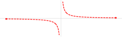
Figure 1: The perturbed branch cut starting from $\pm\tilde{k}_{l}$ where $\tilde{k}_{l}=k_{l}+\epsilon_{l}{\mathrm{i}}$

Let $\lambda_{\nu}$ be a real pole of $\sigma_{ts}^{\ast\star}(\lambda)$ in the integrand of Eq. 11, which is known as a surface wave pole [10, 11]. Integration across the surface wave pole is understood as the limiting case of the perturbed system with lossy media as mentioned above. For simplicity, suppose $\sigma_{ts}^{\ast\star}(\lambda)=\sigma(\lambda;k_{1},\cdots,k_{L})$ is the limit of the perturbed field $\sigma(\lambda;\tilde{k}_{1},\cdots,\tilde{k}_{L})$ with pole $\tilde{\lambda}_{\nu}$, and $\tilde{\lambda}_{\nu}\rightarrow\lambda_{\nu}\in(a,b)$ as all the $\epsilon_{l}\rightarrow 0^{+}$. Let $\sigma_{\nu}=\lim_{\lambda\rightarrow\lambda_{\nu}}\sigma(\lambda)(\lambda-\lambda_{\nu})$. Given any smooth function $h(\lambda)$, the limiting integral $\int_{a}^{b}h(\lambda)\sigma(\lambda)d\lambda$ is evaluated by the formula

(14) $$\int_{a}^{b}h(\lambda)\sigma(\lambda;\tilde{k}_{1},\cdots,\tilde{k}_{L})d\lambda\to \int_{a}^{b}\left(h(\lambda)\sigma(\lambda)-\frac{h(\lambda_{\nu})\sigma_{\nu}}{\lambda-\lambda_{\nu}}\right)d\lambda$$

$$+\mathrm{p.v.}\int_{a}^{b}\frac{h(\lambda_{\nu})\sigma_{\nu}}{\lambda-\lambda_{\nu}}d\lambda\pm{\mathrm{i}}\pi h(\lambda_{\nu})\sigma_{\nu},$$

here the $\pm$ sign is positive (or negative) when the perturbed pole $\tilde{\lambda}_{\nu}\rightarrow\lambda_{\nu}$ from the upper (or the lower) half of the complex plane, and the principal value part vanishes if $(a,b)=(-\infty,+\infty)$.

In a well-posed physical problem, the poles will be at most of order one, and $\tilde{\lambda}_{\nu}$ should keep in one side of the half planes as all the perturbation parameters $\epsilon_{l}$ are sufficiently small, otherwise the limit of the integral does not exist and the field is not well-defined. Also, $0$ can not be a surface wave pole, otherwise the surface wave does not propagate [10, 11].

Remark 2.5.

Modes of the layered system are classified as the radiation modes, the guided modes (corresponding to the real poles) and the leaky modes (corresponding to other complex poles) [10].

2.4 The far-field expansions and their exponential convergence

Here, we derive the far-field expansions for each integral $u_{ts}^{\ast\star}\left(\mathbf{x},\mathbf{x}^{\prime};\sigma_{ts}^{\ast\star}\right)$ in a natural generalization of the free-space case discussed in Section 2.2, then show their exponential convergence. The derivation relies on the following two types of series expansions.

Suppose $(\rho_{0},\theta_{0})$ are the polar coordinates of $(x_{0},y_{0})$. Denote

(15) $$w_{l}(\lambda)=\frac{\lambda-\sqrt{\lambda^{2}-k_{l}^{2}}}{k_{l}},\text{ }0\leq l\leq L.$$

By using the Bessel generating function Eq. 1, we have

(16) $$\begin{split}e^{-\sqrt{\lambda^{2}-k_{s}^{2}}\tau^{\star}y_{0}-{\mathrm{i}}\lambda x_{0}}={}&g\left(k_{s}\rho_{0},-{\mathrm{i}}e^{{\mathrm{i}}\tau^{\star}\theta_{0}}w_{s}(\lambda)\right)\\ ={}&\sum_{p=-\infty}^{\infty}J_{p}(k_{s}\rho_{0})e^{{\mathrm{i}}p\tau^{\star}\theta_{0}}\cdot\left(-{\mathrm{i}}w_{s}(\lambda)\right)^{p},\end{split}$$

(17) $$\begin{split}e^{-\sqrt{\lambda^{2}-k_{t}^{2}}\tau^{\ast}y_{0}+{\mathrm{i}}\lambda x_{0}}={}&g\left(k_{t}\rho_{0},{\mathrm{i}}e^{{\mathrm{i}}\tau^{\ast}\theta_{0}}w_{t}(\lambda)^{-1}\right)\\ ={}&\sum_{m=-\infty}^{\infty}J_{m}(k_{s}\rho_{0})e^{{\mathrm{i}}m\tau^{\ast}\theta_{0}}\cdot\left({\mathrm{i}}w_{t}(\lambda)^{-1}\right)^{m}.\end{split}$$

For the ME, we split the difference $\mathbf{x}-\mathbf{x}^{\prime}=\left(\mathbf{x}-\mathbf{x}_{c}\right)+\left(\mathbf{x}_{c}-\mathbf{x}^{\prime}\right)$, namely, we shift the source $\mathbf{x}^{\prime}$ to a common source center $\mathbf{x}_{c}=(x_{c},y_{c})$ (assumed to be on the same side of the interface $y=d_{s}^{\star}$, i.e. $y_{c}-d_{s}^{\star}$ and $y^{\prime}-d_{s}^{\star}$ have the same sign). Let $(\rho_{c}^{\prime},\theta_{c}^{\prime})$ be the polar coordinates of $\mathbf{x}^{\prime}-\mathbf{x}_{c}$. Using Eq. 16 with $(\rho_{0},\theta_{0})=(\rho_{c}^{\prime},\theta_{c}^{\prime})$ and the separability of the plane wave factor $\mathcal{E}_{ts}^{\star\star}(\mathbf{x},\mathbf{x}^{\prime})$ (11), we get an approximation,

(18) $$u_{ts}^{\ast\star}\left(\mathbf{x},\mathbf{x}^{\prime};\sigma_{ts}^{\ast\star}\right) =\int_{-\infty}^{\infty}\mathcal{E}_{ts}^{\ast\star}(\mathbf{x},\mathbf{x}^{\prime},\lambda)\sigma_{ts}^{\ast\star}(\lambda)d\lambda$$

$$=\int_{-\infty}^{\infty}\mathcal{E}_{ts}^{\ast\star}(\mathbf{x},\mathbf{x}_{c},\lambda)\sigma_{ts}^{\ast\star}(\lambda)e^{-\sqrt{\lambda^{2}-k_{s}^{2}}\tau^{\star}(y^{\prime}-y_{c})+{\mathrm{i}}\lambda(x_{c}-x^{\prime})}d\lambda$$

$$=\int_{-\infty}^{\infty}\mathcal{E}_{ts}^{\ast\star}(\mathbf{x},\mathbf{x}_{c},\lambda)\sigma_{ts}^{\ast\star}(\lambda)\sum_{p=-\infty}^{\infty}J_{p}(k_{s}\rho_{c}^{\prime})e^{{\mathrm{i}}p\tau^{\star}\theta_{c}^{\prime}}\left(-{\mathrm{i}}w_{s}(\lambda)\right)^{p}d\lambda$$

$$\approx\sum_{|p|<P}I_{p}^{\ast\star}(\mathbf{x},\mathbf{x}_{c})M_{p}^{\star}(\mathbf{x}^{\prime},\mathbf{x}_{c})$$

where the expansion function

(19) $$I_{p}^{\ast\star}(\mathbf{x},\mathbf{x}_{c})=\int_{-\infty}^{\infty}\mathcal{E}_{ts}^{\ast\star}(\mathbf{x},\mathbf{x}_{c},\lambda)\sigma_{ts}^{\ast\star}(\lambda)\left(-{\mathrm{i}}w_{s}(\lambda)\right)^{p}d\lambda,$$

and the ME cofficient

(20) $$M_{p}^{\star}(\mathbf{x}^{\prime},\mathbf{x}_{c})=J_{p}(k_{s}\rho_{c}^{\prime})e^{{\mathrm{i}}p\tau^{\star}\theta_{c}^{\prime}}.$$

For LE, we split the difference $\mathbf{x}-\mathbf{x}^{\prime}=\left(\mathbf{x}-\mathbf{x}_{c}^{l}\right)+\left(\mathbf{x}_{c}^{l}-\mathbf{x}^{\prime}\right)$, namely, we shift the target $\mathbf{x}$ to a common target (local) center $\mathbf{x}_{c}^{l}=(x_{c}^{l},y_{c}^{l})$ (assumed to be on the same side of the interface $y=d_{t}^{\ast}$). Let $(\rho^{l},\theta^{l})$ be the polar coordinates of $\mathbf{x}-\mathbf{x}_{c}^{l}$. Using Eq. 17 with $(\rho_{0},\theta_{0})=(\rho^{l},\theta^{l})$ and the separability of the plane wave factor $\mathcal{E}_{ts}^{\star\star}(\mathbf{x},\mathbf{x}^{\prime})$ (11), we get an approximation,

(21) $$u_{ts}^{\ast\star}\left(\mathbf{x},\mathbf{x}^{\prime};\sigma_{ts}^{\ast\star}\right)$$

$$= \int_{-\infty}^{\infty}\mathcal{E}_{ts}^{\ast\star}(\mathbf{x}_{c}^{l},\mathbf{x}^{\prime},\lambda)\sigma_{ts}^{\ast\star}(\lambda)\sum_{m=-\infty}^{\infty}J_{m}(k_{t}\rho^{l})e^{{\mathrm{i}}m\tau^{\ast}\theta^{l}}\cdot\left({\mathrm{i}}w_{t}(\lambda)^{-1}\right)^{m}d\lambda$$

$$\approx \sum_{|m|<M}L_{m}^{\ast\star}(\mathbf{x}_{c}^{l},\mathbf{x}^{\prime})K_{m}^{\ast}(\mathbf{x},\mathbf{x}_{c}^{l})$$

where the expansion function

(22) $$K_{m}^{\ast}(\mathbf{x},\mathbf{x}_{c}^{l})=J_{m}(k_{t}\rho^{l})e^{{\mathrm{i}}m\tau^{\ast}\theta^{l}},$$

and the LE coefficient

(23) $$L_{m}^{\ast\star}(\mathbf{x}_{c}^{l},\mathbf{x}^{\prime})=\int_{-\infty}^{\infty}\mathcal{E}_{ts}^{\ast\star}(\mathbf{x}_{c}^{l},\mathbf{x}^{\prime},\lambda)\sigma_{ts}^{\ast\star}(\lambda)\left({\mathrm{i}}w_{t}(\lambda)^{-1}\right)^{m}d\lambda.$$

The M2L can be derived directly by using the splitting $\mathbf{x}_{c}^{l}-\mathbf{x}^{\prime}=\left(\mathbf{x}_{c}^{l}-\mathbf{x}_{c}\right)+\left(\mathbf{x}_{c}-\mathbf{x}^{\prime}\right)$ in $L_{m}^{\ast\star}(\mathbf{x}_{c}^{l},\mathbf{x}^{\prime})$,

(24) $$L_{m}^{\ast\star}(\mathbf{x}_{c}^{l},\mathbf{x}^{\prime})$$

$$= \int_{-\infty}^{\infty}\mathcal{E}_{st}^{\ast\star}(\mathbf{x}_{c}^{l},\mathbf{x}_{c},\lambda)\sigma_{st}^{\ast\star}(\lambda)\left({\mathrm{i}}w_{t}(\lambda)^{-1}\right)^{m}\sum_{p=-\infty}^{\infty}J_{p}(k_{s}\rho_{c}^{\prime})e^{{\mathrm{i}}p\tau^{\star}\theta_{c}^{\prime}}\cdot\left(-{\mathrm{i}}w_{s}(\lambda)\right)^{p}d\lambda$$

$$\approx \sum_{|p|<P}A_{mp}^{\ast\star}(\mathbf{x}_{c}^{l},\mathbf{x}_{c})M_{p}^{\star}(\mathbf{x}^{\prime},\mathbf{x}_{c}).$$

where the translation coefficients $A_{mp}^{\ast\star}(\mathbf{x}_{c}^{l},\mathbf{x}_{c})$ are given by

$$A_{mp}^{\ast\star}(\mathbf{x}_{c}^{l},\mathbf{x}_{c})=\int_{-\infty}^{\infty}\mathcal{E}_{ts}^{\ast\star}(\mathbf{x}_{c}^{l},\mathbf{x}_{c},\lambda)\sigma_{ts}^{\ast\star}(\lambda)\left(-{\mathrm{i}}w_{s}(\lambda)\right)^{p}\left({\mathrm{i}}w_{t}(\lambda)^{-1}\right)^{m}d\lambda.$$

The L2L shifts the local center $\mathbf{x}_{c}^{l}$ in each integral $L_{m}^{\ast\star}(\mathbf{x}_{c}^{l},\mathbf{x}^{\prime})$ to a new local center $\tilde{\mathbf{x}}_{c}^{l}=(\tilde{x}_{c}^{l},\tilde{y}_{c}^{l})$. Let $(\tilde{\rho},\tilde{\theta})$ be the polar coordinates of $\tilde{\mathbf{x}}_{c}^{l}-\mathbf{x}_{c}^{l}$. Using Eq. 17 with $(\rho_{0},\theta_{0})=(\tilde{\rho},\tilde{\theta})$,

(25) $$L_{m}^{\ast\star}(\tilde{\mathbf{x}}_{c}^{l},\mathbf{x}^{\prime})$$

$$= \int_{-\infty}^{\infty}\mathcal{E}_{ts}^{\ast\star}(\mathbf{x}_{c}^{l},\mathbf{x}^{\prime},\lambda)\sigma_{ts}^{\ast\star}(\lambda)\left({\mathrm{i}}w_{t}(\lambda)^{-1}\right)^{m}\sum_{p=-\infty}^{\infty}J_{p}(k_{t}\tilde{\rho})e^{{\mathrm{i}}p\tau^{\ast}\tilde{\theta}}\cdot\left({\mathrm{i}}w_{t}(\lambda)^{-1}\right)^{p}d\lambda$$

$$\approx \sum_{|p+m|<P}J_{p}(k_{t}\tilde{\rho})e^{{\mathrm{i}}p\tau^{\ast}\tilde{\theta}}\int_{-\infty}^{\infty}\mathcal{E}_{ts}^{\ast\star}(\mathbf{x}_{c}^{l},\mathbf{x}^{\prime},\lambda)\sigma_{ts}^{\ast\star}(\lambda)\left({\mathrm{i}}w_{t}(\lambda)^{-1}\right)^{m}\left({\mathrm{i}}w_{t}(\lambda)^{-1}\right)^{p}d\lambda$$

$$= \sum_{|p|<P}L_{p}^{\ast\star}(\mathbf{x}_{c}^{l},\mathbf{x}^{\prime})K_{p-m}^{\ast}(\tilde{\mathbf{x}}_{c}^{l},\mathbf{x}_{c}^{l}).$$

Next, before we present the main result of this paper on the convergence of the series expansions above, we introduce the concept of “polarized distance” unique to the interaction in layered media. Given layer indices $s$, $t$ and direction marks $\ast,\star\in\{\uparrow,\downarrow\}$, for points $\mathbf{x}_{1}=(x_{1},y_{1})$ and $\mathbf{x}_{2}=(x_{2},y_{2})$, a “polarized distance” is defined as

(26) $$D_{ts}^{\ast\star}(\mathbf{x}_{1},\mathbf{x}_{2})=\sqrt{(x_{1}-x_{2})^{2}+\left(\tau^{\ast}(y_{1}-d_{t}^{\ast})+\tau^{\star}(y_{2}-d_{s}^{\star})\right)^{2}},$$

provided both $\tau^{\ast}(y_{1}-d_{t}^{\ast})>0$ and $\tau^{\star}(y_{2}-d_{s}^{\star})>0$. (Note that they are not symmetric with respect to $\mathbf{x}_{1}$ and $\mathbf{x}_{2}$.)

Theorem 2.6 (exponential convergence of far-field expansions in layered media).

Suppose the integral $u_{ts}^{\ast\star}\left(\mathbf{x},\mathbf{x}^{\prime};\sigma_{ts}^{\ast\star}\right)$ is derived from a well-posed Helmholtz problem in layered media as in Proposition 2.3. Then, we have the truncation error of ME Eq. 18

(27) $$\left|u_{ts}^{\ast\star}\left(\mathbf{x},\mathbf{x}^{\prime};\sigma_{ts}^{\ast\star}\right)-\sum_{|p|<P}I_{p}^{\ast\star}(\mathbf{x},\mathbf{x}_{c})M_{p}^{\star}(\mathbf{x}^{\prime},\mathbf{x}_{c})\right|\leq c^{\mathrm{ME}}(P)\left(\frac{|\mathbf{x}^{\prime}-\mathbf{x}_{c}|}{D_{ts}^{\ast\star}(\mathbf{x},\mathbf{x}_{c})}\right)^{P},$$

the truncation error of LE Eq. 21

(28) $$\left|u_{ts}^{\ast\star}\left(\mathbf{x},\mathbf{x}^{\prime};\sigma_{ts}^{\ast\star}\right)-\sum_{|m|<M}L_{m}^{\ast\star}(\mathbf{x}_{c}^{l},\mathbf{x}^{\prime})K_{m}^{\ast}(\mathbf{x},\mathbf{x}_{c}^{l})\right|\leq c^{\mathrm{LE}}(M)\left(\frac{|\mathbf{x}-\mathbf{x}_{c}^{l}|}{D_{ts}^{\ast\star}(\mathbf{x}_{c}^{l},\mathbf{x}^{\prime})}\right)^{M},$$

the truncation error of M2L Eq. 24 for each LE coefficient

(29) $$\left|L_{m}^{\ast\star}(\mathbf{x}_{c}^{l},\mathbf{x}^{\prime})-\sum_{|p|<P}A_{mp}^{\ast\star}(\mathbf{x}_{c}^{l},\mathbf{x}_{c})M_{p}^{\star}(\mathbf{x}^{\prime},\mathbf{x}_{c})\right|\leq c^{\mathrm{M2L}}_{m}(P)\left(\frac{|\mathbf{x}^{\prime}-\mathbf{x}_{c}|}{D_{ts}^{\ast\star}(\mathbf{x}_{c}^{l},\mathbf{x}_{c})}\right)^{P}$$

and the truncation error of L2L Eq. 25 for each LE coefficient

(30) $$\left|L_{m}^{\ast\star}(\tilde{\mathbf{x}}_{c}^{l},\mathbf{x}^{\prime})-\sum_{|p|<P}L_{p}^{\ast\star}(\mathbf{x}_{c}^{l},\mathbf{x}^{\prime})K_{p-m}^{\ast}(\tilde{\mathbf{x}}_{c}^{l},\mathbf{x}_{c}^{l})\right|\leq c^{\mathrm{L2L}}_{m}(P)\left(\frac{|\tilde{\mathbf{x}}_{c}^{l}-\mathbf{x}_{c}^{l}|}{D_{ts}^{\ast\star}(\mathbf{x}_{c}^{l},\mathbf{x}^{\prime})}\right)^{P}$$

for some functions $c^{\mathrm{ME}}(\cdot)$, $c^{\mathrm{LE}}(\cdot)$, $c_{m}^{\mathrm{M2L}}(\cdot)$ and $c_{m}^{\mathrm{L2L}}(\cdot)$ having polynomial growth rates, provided that for some given $c_{0}>1$, the far-field conditions

(31) $$\begin{split}D_{ts}^{\ast\star}(\mathbf{x},\mathbf{x}_{c})>c_{0}|\mathbf{x}^{\prime}-\mathbf{x}_{c}|,&\quad D_{ts}^{\ast\star}(\mathbf{x}_{c}^{l},\mathbf{x}^{\prime})>c_{0}|\mathbf{x}-\mathbf{x}_{c}^{l}|,\\ \text{ }D_{ts}^{\ast\star}(\mathbf{x}_{c}^{l},\mathbf{x}_{c})>c_{0}|\mathbf{x}^{\prime}-\mathbf{x}_{c}|,&\quad D_{ts}^{\ast\star}(\mathbf{x}_{c}^{l},\mathbf{x}^{\prime})>c_{0}|\tilde{\mathbf{x}}_{c}^{l}-\mathbf{x}_{c}^{l}|\end{split}$$

hold, respectively. If all the sources, targets and the centers involved above are bounded by a given box, the distances from every center to its nearby interface have a given nonzero lower bound, and there exist $0<\rho_{m}\leq\rho_{M}$ such that

$$\rho_{m}\leq D_{ts}^{\ast\star}(\mathbf{x},\mathbf{x}_{c}),D_{ts}^{\ast\star}(\mathbf{x}_{c}^{l},\mathbf{x}^{\prime}),D_{ts}^{\ast\star}(\mathbf{x}_{c}^{l},\mathbf{x}_{c}),D_{ts}^{\ast\star}(\mathbf{x}_{c}^{l},\mathbf{x}^{\prime})\leq\rho_{M},$$

then the functions $c^{\mathrm{ME}}(\cdot)$, $c^{\mathrm{LE}}(\cdot)$, $c_{m}^{\mathrm{M2L}}(\cdot)$ and $c_{m}^{\mathrm{L2L}}(\cdot)$ can be chosen to be determined by these bounds, without dependence on the actual positions of the source locations.

The proof will be a special case of a more general convergence result of the Bessel-type expansions in Theorem 3.14, to be given in Section 3.

2.5 Implementation of a FMM framework for sources in layered media

In the far-field conditions Eq. 31 of the convergence results, the polarized distances $D_{ts}^{\ast\star}$ play the role of the far-field distances as in the free-space cases, which will affect how the ME based FMM will be implemented.

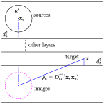
(a)

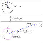
(b)

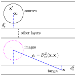
(c)

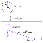
(d)

Figure 2: The far-field distance $\rho_{c}$ of the ME in various field propagation directions.

Define a bijective linear mapping

(32) $$\mathcal{P}_{ts}^{\ast\star}:\mathbf{x}_{2}=(x_{2},y_{2})\mapsto\tilde{\mathbf{x}}_{2}=\left(x_{2},d_{t}^{\ast}-\tau^{\ast}\tau^{\star}\left(y_{2}-d_{s}^{\star}\right)\right)$$

provided $\tau^{\star}\left(y_{2}-d_{s}^{\star}\right)>0$. It is straightforward that

(33) $$D_{ts}^{\ast\star}(\mathbf{x}_{1},\mathbf{x}_{2})=\left\|\mathbf{x}_{1}-\mathcal{P}_{ts}^{\ast\star}(\mathbf{x}_{2})\right\|,$$

here $\|\cdot\|$ is the Euclidean norm. Figure 2 shows how $\mathcal{P}_{ts}^{\ast\star}$ maps the sources to their “polarization images” and the far-field distance of the ME should be $D_{ts}^{\ast\star}(\mathbf{x},\mathbf{x}_{c})$ for various reaction component of the Green’s function.

The FMM for layered media can be set up to evaluate each reaction component $u_{ts}^{\ast\star}$ as follows: $\mathcal{P}_{ts}^{\ast\star}$ maps the source layer $s$ to a neighboring layer (below or above) of the target layer $t$, where all the far-field distances become Euclidean as in Eq. 33. Therefore, to calculate the interaction due to any of the reaction component $u_{ts}^{\ast\star}\left(\mathbf{x},\mathbf{x}^{\prime};\sigma_{ts}^{\ast\star}\right)$, we simply move the source charges to the locations of their corresponding “polarization images”. An implementation for Helmholtz equations in 3-D layered media based on this approach is given in [9].

3 The convergence estimate on Bessel-type expansions

In this section, we will give convergence estimates on general Bessel-type expansions, of which Theorem 2.6 will be a special case.

The Bessel-type expansions are defined as follows. Let $k>0$, $(\rho,\theta)$, $(\rho^{\prime},\theta^{\prime})$ be the polar coordinates of $\mathbf{x}=(x,y)$ and $\mathbf{x}^{\prime}=(x^{\prime},y^{\prime})$, respectively. Suppose $y>0$, $y+y^{\prime}>0$ and $\rho>\rho^{\prime}\geq 0$. For simplicity, define

(34) $$\Psi(\lambda)\equiv\Psi(\mathbf{x,}\lambda)=e^{-\sqrt{\lambda^{2}-k^{2}}y+{\mathrm{i}}\lambda x},\quad\Psi^{\prime}(\lambda)\equiv\Psi^{\prime}(\mathbf{x}^{\prime}\mathbf{,}\lambda)=e^{-\sqrt{\lambda^{2}-k^{2}}y^{\prime}-{\mathrm{i}}\lambda x^{\prime}}.$$

Then, we claim the pointwise Bessel-type expansion for a given $\lambda_{\nu}\in\mathbb{C}$,

(35) $$e^{-\sqrt{\lambda_{\nu}^{2}-k^{2}}(y+y^{\prime})+{\mathrm{i}}\lambda_{\nu}(x-x^{\prime})}=\sum_{p=-\infty}^{\infty}J_{p}(k\rho^{\prime})e^{{\mathrm{i}}p\theta^{\prime}}\Psi(\mathbf{x,}\lambda_{\nu})\left(-{\mathrm{i}}w(\lambda_{\nu})\right)^{p}$$

and the integral Bessel-type expansion for the integration over $\lambda\in[a,b],-\infty\leq a<b\leq+\infty,$

(36) $$\int_{a}^{b}e^{-\sqrt{\lambda^{2}-k^{2}}(y+y^{\prime})+{\mathrm{i}}\lambda(x-x^{\prime})}f(\lambda)d\lambda=\sum_{p=-\infty}^{\infty}J_{p}(k\rho^{\prime})e^{{\mathrm{i}}p\theta^{\prime}}F_{p}(x,y),$$

where $f(\lambda)$ is a complex function defined on $(a,b)$ satisfying certain conditions to be specified later, and $F_{p}(x,y)$ is the expansion function

$$F_{p}(x,y)=\int_{a}^{b}\Psi(\mathbf{x,}\lambda)\left(-{\mathrm{i}}w(\lambda)\right)^{p}f(\lambda)d\lambda.$$

3.1 Convergence of pointwise Bessel-type expansions

We first present the convergence of Eq. 35.

Lemma 3.1.

Let $c_{0}>1$, $k>0$. Suppose $(\rho^{\prime},\theta^{\prime})$ are the polar coordinates of $(x^{\prime},y^{\prime})$, $x\in\mathbb{R}$, $y\in\mathbb{R}^{+}$ satisfying $\rho=\sqrt{x^{2}+y^{2}}>c_{0}\rho^{\prime}\geq 0$ and $x\cdot\Im\lambda_{\nu}\geq 0$. Then, the Bessel-type expansion Eq. 35 holds with a truncation error estimate

(37) $$\left|\sum_{|p|\geq P}J_{p}(k\rho^{\prime})e^{{\mathrm{i}}p\theta^{\prime}}\Psi(\mathbf{x,}\lambda_{\nu})\left(-{\mathrm{i}}w(\lambda_{\nu})\right)^{p}\right|\leq\frac{2c_{0}}{c_{0}-1}\left(\frac{\rho^{\prime}}{\rho}\right)^{P}$$

for any $P\geq e(|\lambda_{\nu}|+k/2)\rho$.

Proof 3.2.

The equality of Eq. 35 is given by the Bessel generating function Eq. 1

(38) $$\begin{split}e^{-\sqrt{\lambda_{\nu}^{2}-k^{2}}(y+y^{\prime})+{\mathrm{i}}\lambda_{\nu}(x-x^{\prime})}&=\Psi(\lambda_{\nu})g\left(k\rho^{\prime},-{\mathrm{i}}e^{{\mathrm{i}}\theta^{\prime}}w(\lambda_{\nu})\right)\\ &=\text{ }\sum_{p=-\infty}^{\infty}J_{p}(k\rho^{\prime})e^{{\mathrm{i}}p\theta^{\prime}}\mathcal{E}(\lambda_{\nu})\left(-{\mathrm{i}}w(\lambda_{\nu})\right)^{p}.\end{split}$$

With the given conditions, $|\exp({-\sqrt{\lambda_{\nu}^{2}-k^{2}}y+{\mathrm{i}}\lambda_{\nu}x})|\leq 1$, $|w(\lambda_{\nu})|\leq(2|\lambda_{\nu}|+k)/{k}$, hence for each $p$, using Lemma 2.1,

$$\left|J_{p}(k\rho^{\prime})e^{{\mathrm{i}}p\theta^{\prime}}e^{-\sqrt{\lambda_{\nu}^{2}-k^{2}}y+{\mathrm{i}}\lambda_{\nu}x}\left(-{\mathrm{i}}w(\lambda_{\nu})\right)^{p}\right|\leq\frac{1}{|p|!}\left(\frac{k\rho^{\prime}}{2}\right)^{|p|}\left(\frac{2|\lambda_{\nu}|+k}{k}\right)^{|p|}.$$

For $|p|\geq e(|\lambda_{\nu}|+k/2)\rho$, using Stirling’s formula [5],

$$|p|!\geq\left(\frac{|p|}{e}\right)^{|p|}\geq\left(\left(|\lambda_{\nu}|+\frac{k}{2}\right)\rho\right)^{|p|},$$

thus,

$$\left|J_{p}(k\rho^{\prime})e^{{\mathrm{i}}p\theta^{\prime}}e^{-\sqrt{\lambda_{\nu}^{2}-k^{2}}y+{\mathrm{i}}\lambda_{\nu}x}\left(-{\mathrm{i}}w(\lambda_{\nu})\right)^{p}\right|\leq\left(\frac{\rho^{\prime}}{\rho}\right)^{|p|},$$

which will give the estimate of the truncation error after summing over $|p|\geq P$.

3.2 Special cases of integral Bessel-type expansion

First, we consider Eq. 36 when the integral is defined on a bounded interval $[-k^{\prime},k^{\prime}]$.

Lemma 3.3.

Let $c_{0}>1$, $k^{\prime}\geq k>0$. Let $(\rho,\theta)$ and $(\rho^{\prime},\theta^{\prime})$ be the polar coordinates of $\mathbf{x}=(x,y)$ and $\mathbf{x}^{\prime}=(x^{\prime},y^{\prime})$, respectively. Suppose $y>0$, $\rho>c_{0}\rho^{\prime}\geq 0$, and the function ${f}(\lambda)$ on $[-k^{\prime},k^{\prime}]$ satisfies $\int_{-k^{\prime}}^{k^{\prime}}|{f}(\lambda)|d\lambda=S<+\infty$, then the integral Bessel-type expansion Eq. 36 holds on $[-k^{\prime},k^{\prime}]$ with a truncation error estimate

(39) $$\left|\sum_{|p|\geq P}J_{p}(k\rho^{\prime})e^{{\mathrm{i}}p\theta^{\prime}}F_{p}\right|\leq\frac{2c_{0}S}{c_{0}-1}\left(\frac{\rho^{\prime}}{\rho}\right)^{P}$$

for any $P\geq ek^{\prime}\rho$.

Proof 3.4.

When $|\lambda|\leq k^{\prime}$,

$$\left|e^{-\sqrt{\lambda^{2}-k^{2}}y+{\mathrm{i}}\lambda x}\right|\leq 1,\quad\left|w(\lambda)\right|^{\pm 1}=\left|\frac{\lambda-\sqrt{\lambda^{2}-k^{2}}}{k}\right|^{\pm 1}\leq\frac{2k^{\prime}}{k},$$

so each $F_{p}$ is bounded by

$$|F_{p}|\leq\tilde{F}_{p}:=\int_{-k^{\prime}}^{k^{\prime}}\left|e^{-\sqrt{\lambda^{2}-k^{2}}y+{\mathrm{i}}\lambda x}\left(-{\mathrm{i}}w(\lambda)\right)^{p}f(\lambda)\right|d\lambda\leq S\left(\frac{2k^{\prime}}{k}\right)^{|p|}.$$

When $|p|\geq ek^{\prime}\rho$, using Stirling’s formula [5], $|p|!\geq\left({|p|}/{e}\right)^{|p|}\geq(k^{\prime}\rho)^{|p|}$, so

$$\tilde{F}_{p}\leq S\left(\frac{2k^{\prime}}{k}\right)^{|p|}\leq S|p|!\left(\frac{k\rho}{2}\right)^{-|p|}.$$

Hence for $|p|\geq ek^{\prime}\rho$, by Lemma 2.1,

$$\int_{-k^{\prime}}^{k^{\prime}}\left|J_{p}(k\rho^{\prime})e^{{\mathrm{i}}p\theta^{\prime}}e^{-\sqrt{\lambda^{2}-k^{2}}y+{\mathrm{i}}\lambda x}\left(-{\mathrm{i}}w(\lambda)\right)^{p}f(\lambda)\right|d\lambda\leq\frac{1}{|p|!}\left(\frac{k\rho^{\prime}}{2}\right)^{|p|}\tilde{F}_{p}\leq S\left(\frac{\rho^{\prime}}{\rho}\right)^{|p|}.$$

Similar as in Eq. 38 and using the Fubini’s theorem,

$$\int_{-k^{\prime}}^{k^{\prime}}e^{-\sqrt{\lambda^{2}-k^{2}}(y+y^{\prime})+{\mathrm{i}}\lambda(x-x^{\prime})}f(\lambda)d\lambda =\int_{-k^{\prime}}^{k^{\prime}}{\sum_{p=-\infty}^{\infty}J_{p}(k\rho^{\prime})e^{{\mathrm{i}}p\theta^{\prime}}\Psi(\lambda)\left(-{\mathrm{i}}w(\lambda)\right)^{p}f(\lambda)d\lambda}$$

$$=\sum_{p=-\infty}^{\infty}J_{p}(k\rho^{\prime})e^{{\mathrm{i}}p\theta^{\prime}}F_{p}.$$

For $P\geq ek^{\prime}\rho$, the truncation error

$$\left|\sum_{|p|\geq P}J_{p}(k\rho^{\prime})e^{{\mathrm{i}}p\theta^{\prime}}F_{p}\right|\leq\sum_{|p|\geq P}S\left(\frac{\rho^{\prime}}{\rho}\right)^{|p|}\leq\frac{2c_{0}S}{c_{0}-1}\left(\frac{\rho^{\prime}}{\rho}\right)^{P}.$$

A similar result can be derived for a complex path of finite length.

Lemma 3.5.

Let $c_{0}>1$, $k>0$. Let $(\rho,\theta)$ and $(\rho^{\prime},\theta^{\prime})$ be the polar coordinates of $\mathbf{x}=(x,y)$ and $\mathbf{x}^{\prime}=(x^{\prime},y^{\prime})$, respectively. Suppose $y>0$, $\rho>c_{0}\rho^{\prime}\geq 0$. Let $\kappa\subset\mathbb{C}$ be a smooth curve with length $|\kappa|<+\infty$. Suppose $x\cdot\Im\lambda\geq 0$ for any $\lambda\in\kappa$. Let $f(\lambda)$ be a complex function defined on $\kappa$ satisfying $|f(\lambda)|\leq f_{0}$. Then,

(40) $$E_{\kappa}=\int_{\kappa}\Psi(\lambda)\Psi^{\prime}(\lambda)f(\lambda)d\lambda=\sum_{p=-\infty}^{\infty}J_{p}(k\rho^{\prime})e^{{\mathrm{i}}p\theta^{\prime}}\int_{\kappa}\Psi(\lambda)\left(-{\mathrm{i}}w(\lambda)\right)^{p}f(\lambda)d\lambda,$$

with a truncation error estimate

(41) $$\left|\sum_{|p|\geq P}J_{p}(k\rho^{\prime})e^{{\mathrm{i}}p\theta^{\prime}}\int_{\kappa}\Psi(\lambda)\left(-{\mathrm{i}}w(\lambda)\right)^{p}f(\lambda)d\lambda\right|\leq\frac{2c_{0}f_{0}|\kappa|}{c_{0}-1}\left(\frac{\rho^{\prime}}{\rho}\right)^{P}$$

for any $P\geq e(\lambda_{M}+k/2)\rho$, where $\lambda_{M}=\max_{\lambda\in\kappa}|\lambda|$.

Proof 3.6.

Suppose $\kappa$ is parameterized by $\lambda=a(s)+b(s){\mathrm{i}}$, $s\in[0,1]$, here $a(s)$ and $b(s)$ are real and smooth functions. Using the results from the proof of Lemma 3.1 and Lemma 3.3, for $\lambda\in\kappa$,

$$\left|e^{-\sqrt{\lambda^{2}-k^{2}}y+{\mathrm{i}}\lambda x}\right|\leq 1\text{, }|w(\lambda)|\leq\frac{2\lambda_{M}+k}{k},$$

so for each $p$, using Lemma 2.1,

$$\int_{0}^{1}\left|J_{p}(k\rho^{\prime})e^{{\mathrm{i}}p\theta^{\prime}}\Psi(\lambda)\left(-{\mathrm{i}}w(\lambda)\right)^{p}f(\lambda)\left(a^{\prime}(s)+b^{\prime}(s){\mathrm{i}}\right)\right|ds$$

$$\leq \frac{1}{|p|!}\left(\frac{k\rho^{\prime}}{2}\right)^{p}\cdot 1\cdot\left(\frac{2\lambda_{M}+k}{k}\right)^{p}\cdot f_{0}|\kappa|.$$

Hence, using the Bessel generating function Eq. 1 and the Fubini’s theorem,

$$E_{\kappa}= \int_{0}^{1}\Psi(\lambda)\Psi^{\prime}(\lambda)f(\lambda)\left(a^{\prime}(s)+b^{\prime}(s){\mathrm{i}}\right)ds$$

$$= \sum_{p=-\infty}^{\infty}\int_{0}^{1}J_{p}(k\rho^{\prime})e^{{\mathrm{i}}p\theta^{\prime}}\Psi(\lambda)\left(-{\mathrm{i}}w(\lambda)\right)^{p}f(\lambda)\left(a^{\prime}(s)+b^{\prime}(s){\mathrm{i}}\right)ds$$

$$= \sum_{p=-\infty}^{\infty}\int_{\kappa}J_{p}(k\rho^{\prime})e^{{\mathrm{i}}p\theta^{\prime}}\Psi(\lambda)\left(-{\mathrm{i}}w(\lambda)\right)^{p}f(\lambda)d\lambda,$$

we get the equality of Eq. 40. The truncation error estimate is similar as in the proof of Lemma 3.3, except from replacing $k^{\prime}$ by $\lambda_{M}+k/2$.

Next, we consider a special case when $(x,y)=(0,\rho)$ in the Bessel-type expansion Eq. 36 over an infinite interval.

Lemma 3.7.

Let $c_{0}>1$, $k^{\prime}\geq k>0$, $x^{\prime},y^{\prime}\in\mathbb{R}$, $\rho>c_{0}\rho^{\prime}=\sqrt{x^{\prime 2}+y^{\prime 2}}\geq 0$. Let $C\in\mathbb{R}^{+}$ and $K$ be a nonnegative integer, and

(42) $$E_{p}^{+}=\int_{k^{\prime}}^{\infty}e^{-\sqrt{\lambda^{2}-k^{2}}\rho}\left(-{\mathrm{i}}w(\lambda)\right)^{p}f(\lambda)d\lambda,\text{ }p\in\mathbb{Z},$$

here $f(\lambda)$ satisfies $|f(\lambda)|\leq C\lambda^{K}$ for $\lambda\in[k^{\prime},\infty)$. Then for any sufficiently large $|p|$ such that $|p|\geq(k\rho)^{2}/4+1-K$ we have the estimate

(43) $$\left|E_{p}^{+}\right|\leq\int_{k^{\prime}}^{\infty}e^{-\sqrt{\lambda^{2}-k^{2}}\rho}w(\lambda)^{p}|f(\lambda)|d\lambda\leq 3C\left(|p|+K\right)!\left(\frac{2}{\rho}\right)^{K+1}\left(\frac{k\rho}{2}\right)^{-|p|}.$$

In addition, the Bessel-type expansion Eq. 36 holds with $(x,y)=(0,\rho)$ on the interval $(k^{\prime},\infty)$, with a truncation error estimate

(44) $$\left|\int_{k^{\prime}}^{\infty}e^{-\sqrt{\lambda^{2}-k^{2}}(\rho+y^{\prime})+{\mathrm{i}}\lambda(-x^{\prime})}f(\lambda)d\lambda-\sum_{|p|<P}J_{p}(k\rho^{\prime})e^{{\mathrm{i}}p\theta^{\prime}}E_{p}^{+}\right|\leq c(P)\left(\frac{\rho^{\prime}}{\rho}\right)^{P}$$

for any $P\geq(k\rho)^{2}/4+1-K$, where

(45) $$c(P)=6C(K+1)!\left(\frac{2c_{0}}{\rho(c_{0}-1)}\right)^{K+1}(P+K)^{K}.$$

Proof 3.8.

Notice that for $\lambda\geq k$ we have $\sqrt{\lambda^{2}-k^{2}}\leq\lambda$ and $0\leq\lambda-\sqrt{\lambda^{2}-k^{2}}\leq k\leq\lambda\leq\lambda+\sqrt{\lambda^{2}-k^{2}}$, so each $|E_{p}^{+}|\leq Ck^{K+1}I_{p}$, where

(46) $$I_{p}=\int_{k}^{\infty}\frac{e^{-\sqrt{\lambda^{2}-k^{2}}\rho}}{\sqrt{\lambda^{2}-k^{2}}}\left(\frac{\lambda+\sqrt{\lambda^{2}-k^{2}}}{k}\right)^{M+1}d\lambda,$$

here $M=|p|+K$. With the substitution $v=(\lambda+\sqrt{\lambda^{2}-k^{2}})/k$,

$$I_{p} =\int_{1}^{\infty}e^{\frac{k\rho}{2}(-v+v^{-1})}v^{M}dv$$

$$\leq\int_{1}^{\infty}e^{\frac{k\rho}{2}(-v)}\left(\sum_{j=0}^{M-1}\frac{1}{j!}\left(\frac{k\rho}{2}v^{-1}\right)^{j}+\frac{1}{M!}\left(\frac{k\rho}{2}v^{-1}\right)^{M}e^{\frac{k\rho}{2}v^{-1}}\right)v^{M}dv$$

$$\leq\sum_{j=0}^{M-1}\frac{1}{j!}\left(\frac{k\rho}{2}\right)^{j}\int_{0}^{\infty}e^{\frac{k\rho}{2}(-v)}v^{M-j}dv+\frac{1}{M!}\left(\frac{k\rho}{2}\right)^{M}\int_{1}^{\infty}e^{\frac{k\rho}{2}(-v+1)}dv$$

$$=\sum_{j=0}^{M-1}\frac{(M-j)!}{j!}\left(\frac{k\rho}{2}\right)^{2j-M-1}+\frac{1}{M!}\left(\frac{k\rho}{2}\right)^{M-1}$$

$$=M!\left(\frac{k\rho}{2}\right)^{-M-1}\sum_{j=0}^{M}c_{j}$$

where

(47) $$c_{j}=\frac{(M-j)!}{M!j!}\left(\frac{k\rho}{2}\right)^{2j},\text{ }j=0,\cdots,M.$$

One can quickly verify $c_{0}=1$, $c_{1}=\left({k\rho}/{2}\right)^{2}/M\leq{(M-1)}/{M}$. For $1\leq j\leq M-2$, we have $c_{j+1}/c_{j}=(k\rho)^{2}/4(j+1)(M-j)\leq 1/2$. For $c_{M}$ we have $c_{M}/c_{M-1}=(k\rho)^{2}/4M\leq 1$. In sum, $\sum_{j=0}^{M}c_{j}\leq c_{0}+2c_{1}\leq 1+2(M-1)/M\leq 3$, so

$$|E_{p}^{+}|\leq Ck^{K+1}I_{p}\leq 3Ck^{K+1}M!\left(\frac{k\rho}{2}\right)^{-M-1}\leq 3C\left(|p|+K\right)!\left(\frac{2}{\rho}\right)^{K+1}\left(\frac{k\rho}{2}\right)^{-|p|}.$$

For the expansion Eq. 36 with $(x,y)=(0,\rho)$ on $[k^{\prime},\infty)$, by Lemma 2.1, for each $p$,

$$\int_{k^{\prime}}^{\infty}\left|J_{p}(k\rho^{\prime})e^{{\mathrm{i}}p\theta^{\prime}}e^{-\sqrt{\lambda^{2}-k^{2}}\rho}\left(-{\mathrm{i}}w(\lambda)\right)^{p}f(\lambda)\right|d\lambda$$

$$\leq \text{ }\frac{1}{|p|!}\left(\frac{k\rho^{\prime}}{2}\right)^{|p|}\cdot 3C\left(|p|+K\right)!\left(\frac{2}{\rho}\right)^{K+1}\left(\frac{k\rho}{2}\right)^{-|p|}$$

$$= \text{ }3C\frac{(|p|+K)!}{|p|!}\left(\frac{2}{\rho}\right)^{K+1}\left(\frac{\rho^{\prime}}{\rho}\right)^{|p|}.$$

Similar as in Eq. 38 and using the Fubini’s theorem,

$$\int_{k^{\prime}}^{\infty}e^{-\sqrt{\lambda^{2}-k^{2}}(\rho+y^{\prime})+{\mathrm{i}}\lambda(-x^{\prime})}f(\lambda)d\lambda$$

$$= \int_{k^{\prime}}^{\infty}{\sum_{p=-\infty}^{\infty}J_{p}(k\rho^{\prime})e^{{\mathrm{i}}p\theta^{\prime}}e^{-\sqrt{\lambda^{2}-k^{2}}\rho}\left(-{\mathrm{i}}w(\lambda)\right)^{p}f(\lambda)d\lambda}$$

$$= \sum_{p=-\infty}^{\infty}J_{p}(k\rho^{\prime})e^{{\mathrm{i}}p\theta^{\prime}}E_{p}^{+}.$$

When $P\geq(k\rho)^{2}/4+1-K$, the $P$-term truncation has the truncation error

$$\left|\sum_{|p|\geq P}J_{p}(k\rho^{\prime})e^{{\mathrm{i}}p\theta^{\prime}}E_{p}^{+}\right|\leq\sum_{|p|\geq P}3C\frac{(|p|+K)!}{|p|!}\left(\frac{2}{\rho}\right)^{K+1}\left(\frac{\rho^{\prime}}{\rho}\right)^{|p|}\leq c(P)\left(\frac{\rho^{\prime}}{\rho}\right)^{P}.$$

Remark 3.9.

The bound of $|E_{p}^{+}|$ in Lemma 3.7 is chosen as an analog of the asymptotic behavior of $H_{n}^{(1)}(x)\sim(n-1)!(x/2)^{n}/({\mathrm{i}}\pi)$ for $x>0$ as $n\to\infty$ [6, (9.3.1)].

3.3 Convergence of general integral Bessel-type expansion

In order to obtain the convergence estimate of the integral Bessel-type expansion Eq. 36 on an infinite interval, we will follow two steps. First, the Cagniard–de Hoop transform [3] will be used to convert the general $(x,y)$ case to the $(\rho,0)$ case as discussed in Lemma 3.7, namely, the complex factor $e^{-\sqrt{\lambda^{2}-k^{2}}y+{\mathrm{i}}\lambda x}$ in Eq. 36 is converted to $e^{-\sqrt{\lambda^{2}-k^{2}}\rho}$; Second, we deform the new complex contour of integration to the real axis, see the illustration in Fig. 3.

3.3.1 The Cagniard–de Hoop transform

Given $x$, $y$ and $T\in\mathbb{R}^{+}$ satisfying $x<Ty$. Let $(\rho,\theta)$ be the polar coordinates of $(x,y)$. Let $\beta=\frac{\pi}{2}-\theta\in(0,\frac{\pi}{2})$, then $y+x{\mathrm{i}}=\rho e^{{\mathrm{i}}\beta}$.

Define the open set

(48) $$\Omega=\left\{z\in\mathbb{C}:\Re z>0,z\notin(0,k]\right\}.$$

Define the holomorphic Cagniard–de Hoop mapping $\phi:\Omega\rightarrow\mathbb{C}$ by

(49) $$\phi(z)=z\cos\beta+{\mathrm{i}}\sqrt{z^{2}-k^{2}}\sin\beta.$$

For any positive real $w\in(k,+\infty)$, one can easily verify that an inverse of $\phi$ at $w$ is found in the fourth quadrant as $\phi^{-1}(w)=w\cos\beta-{\mathrm{i}}\sqrt{w^{2}-k^{2}}\sin\beta$. Let

(50) $$\gamma^{+}=\phi\left((k,+\infty)\right)\text{, }\gamma^{-}=\phi^{-1}\left((k,+\infty)\right),$$

then, $\gamma^{+}\cup\gamma^{-}\cup\{k\cos\beta\}$ is the right branch of the hyperbola

(51) $$\Gamma=\left\{a+b{\mathrm{i}}:a,b\in\mathbb{R},\frac{a}{\cos\beta}=\sqrt{\frac{b^{2}}{\sin^{2}\beta}+k^{2}}\right\}$$

with vertex $k\cos\beta$ on the real axis. $\Gamma$ is known as the Cagniard–de Hoop contour. The lines passing the origin with slope $\pm\tan\beta$ are the asymptotes of $\gamma^{\pm}$.

Define regions to the right of $\Gamma$ in the first and the fourth quadrant, respectively, by

(52) $$D^{\pm}=\{z+t:z\in\gamma^{\pm},t\in\mathbb{R}^{+}\}.$$

$D^{\pm}$ are isomorphic as the following lemma shows.

Lemma 3.10.

$\phi|_{D^{-}}$ is a bijection from $D^{-}$ to $D^{+}$ with inverse $\phi^{-1}|_{D^{+}}$ given by

(53) $$\phi^{-1}(w)=w\cos\beta-{\mathrm{i}}\sqrt{w^{2}-k^{2}}\sin\beta.$$

Proof 3.11.

See Appendix A.

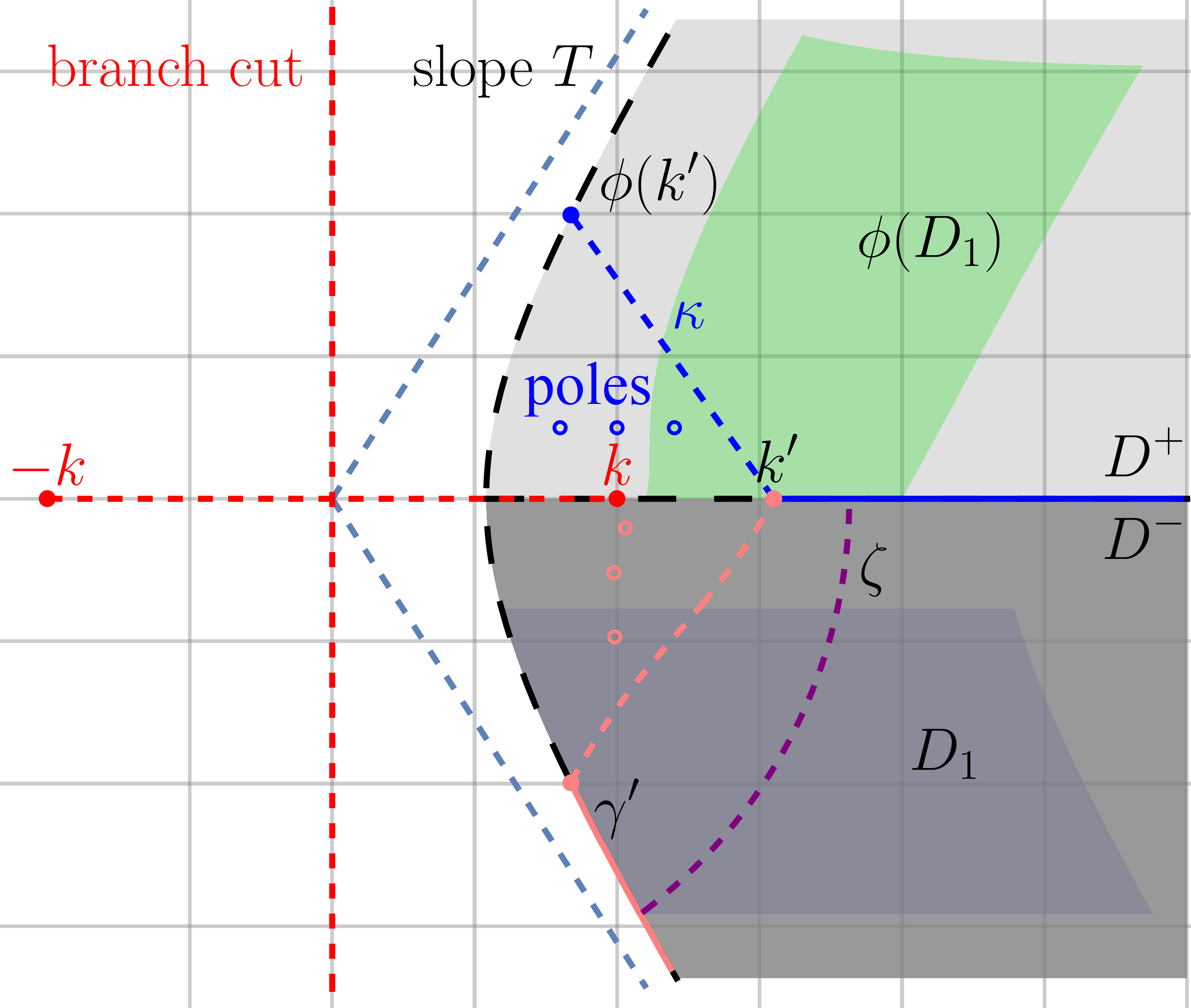
Figure 3: The mapping $\phi$ which maps $D^{-}$ to $D^{+}$. The shadowed region $D_{1}$ is for illustration.

3.3.2 The general Bessel-type expansion

With the above preparation, we can now prove the expansion Eq. 36 when $f(\lambda)$ has a polynomial bound in $\Omega$ when $|\lambda|$ is sufficiently large and $\Im\lambda/\Re\lambda$ is bounded. To make it clear, we make the following assumptions.

Given $T>0$, $\epsilon_{0}>0$. Suppose $f(\lambda)$ is a complex function with branch points $\pm k_{0},\cdots,\pm k_{L}$, it is even and is meromorphic in $\mathbb{C}$ excluding the branch cuts of $\sqrt{\lambda^{2}-k_{l}^{2}}$, $0\leq l\leq L$, with poles of order up to one. Assume that

• $f(\lambda)$ has a decomposition

  (54) $$f(\lambda)=\sum_{r=1}^{n_{r}}\frac{f_{r}}{\lambda-\lambda_{r}}+\bar{f}(\lambda)\text{, and }\bar{f}(\lambda)=\sum_{c=1}^{n_{c}}\frac{f_{c}}{\lambda-\lambda_{c}}+\bar{\bar{f}}(\lambda),$$

  here $\lambda_{r}\neq 0$ are all the real poles of $f(\lambda)$ with residue $f_{r}$, $\lambda_{c}$ are all the (complex) poles of $f(\lambda)$ in the region $\Omega_{T}^{+}=\{a+b{\mathrm{i}}:a>0,0<b<aT\}$ with residue $f_{c}$, respectively, and are bounded by $\lambda_{M}=\max_{1\leq c\leq n_{c}}|\lambda_{c}|$.

• $\left|\bar{\bar{f}}(\lambda)\right|\leq C\left(1+|\lambda|^{K}\right)$ for any $\lambda\in\Omega_{T}^{+}\cup\mathbb{R}^{+}$ satisfying $\max_{0\leq l\leq L}|\lambda-k_{l}|\geq\epsilon_{0}$, here $C>0$ and $K\in\mathbb{N}\cup\{0\}$ are given constants.

• For $k^{\prime}=4k_{M}+2\lambda_{M}+2\epsilon_{0}$, the integral $S=\int_{-k^{\prime}}^{k^{\prime}}\left|\bar{f}(\lambda)\right|d\lambda<+\infty$.

Lemma 3.12.

Let $c_{0}>1$, $T>0$, $\epsilon_{0}>0$ be some given constants. Let $k_{1},\cdots,k_{L}$ be given wave numbers of the layers with maximum $k_{M}$, and $k$ is one of the wave numbers. Suppose the function ${f}(\lambda)$ is given satisfying Section 3.3.2, and $\bar{f}(\lambda)$ is so defined with the real poles removed from $f(\lambda)$, $(\rho,\theta)$ and $(\rho^{\prime},\theta^{\prime})$ are the polar coordinates of $(x,y)$ and $(x^{\prime},y^{\prime})$, respectively, and $\rho>c_{0}\rho^{\prime}\geq 0$. Suppose $y>0$, $y+y^{\prime}>0$ and $|x|<Ty$. Then, the integral Bessel-type expansion Eq. 36 holds (by replacing the original $f(\lambda)$) with $\bar{f}(\lambda)$ on the interval $(k^{\prime},\infty)$, with the truncation error estimate for a finite $P$-term truncation

(55) $$\left|\sum_{|p|\geq P}J_{p}(k\rho^{\prime})e^{{\mathrm{i}}p\theta^{\prime}}\int_{k^{\prime}}^{\infty}\Psi(\lambda)\left(-{\mathrm{i}}w(\lambda)\right)^{p}\bar{f}(\lambda)d\lambda\right|\leq c_{+}(P)\left(\frac{\rho^{\prime}}{\rho}\right)^{P}$$

for any sufficiently large $P\geq m_{+}(\rho)$, here $m_{+}(\rho)$ is an (at most) quadratic function of $\rho$, and $c_{+}(\cdot)$ is a function with polynomial growth rate.

Proof 3.13.

If $x=0$, then $y=\sqrt{x^{2}+y^{2}}=\rho$, and

$$|\bar{f}(\lambda)|\leq C\left(1+|\lambda|^{K}\right)+\sum_{c=1}^{n_{c}}\frac{|f_{c}|}{\Im\lambda_{c}}\leq C_{1}\left(1+|\lambda|^{K}\right)$$

for any $\lambda\in(k^{\prime},\infty)$, here $C_{1}>0$ is a constant number. By Lemma 3.7, we can choose

$$m(\rho)=\left(\frac{k\rho}{2}\right)^{2}+1-K,\quad c_{+}(P)=6C_{1}(K+1)!\left(\frac{2c_{0}}{\rho(c_{0}-1)}\right)^{K+1}(P+K)^{K}.$$

If $x\neq 0$, without loss of generality assume $x>0$, since the $x<0$ case will follow by taking complex conjugates. Let $\beta=\frac{\pi}{2}-\theta$, then $\tan\beta\in(0,T)$. Let $\kappa$ be the segment from $\phi(k^{\prime})$ to $k^{\prime}$ (see Fig. 3). One can verify the length of $\kappa$ is bounded by $\sqrt{2}k^{\prime}$, and that $\lambda_{M}+k_{M}\leq|\lambda|\leq\sqrt{2}k^{\prime}$ and $|\lambda-k_{l}|>\epsilon_{0}$ for $\forall\lambda\in\kappa$ and $\forall 0\leq l\leq L$. Define

(56) $$E=\int_{\kappa\cup(k^{\prime},\infty)}\Psi(\lambda)\Psi^{\prime}(\lambda)\bar{f}(\lambda)d\lambda,\quad G=\int_{\kappa}\Psi(\lambda)\Psi^{\prime}(\lambda)\bar{f}(\lambda)d\lambda,$$

we will discuss the expansions on $E$ and on $G$, separately, then give the integral Bessel-type expansion for $E-G$. For $G$, on $\kappa$ we have the bound of $\bar{f}(\lambda)$ by

(57) $$|\bar{f}(\lambda)|\leq C\left(1+|\lambda|^{K}\right)+\sum_{n=1}^{n_{c}}\frac{|f_{c}|}{|\lambda-\lambda_{c}|}\leq C\left(1+(\sqrt{2}k^{\prime})^{K}\right)+\sum_{c=1}^{n_{c}}\frac{|f_{c}|}{k_{M}}:=C_{2},$$

so by Lemma 3.5, the Bessel-type expansion on $\kappa$ is given by

(58) $$G=\sum_{p=-\infty}^{\infty}J_{p}(k\rho^{\prime})e^{{\mathrm{i}}p\theta^{\prime}}G_{p},\quad G_{p}=\int_{\kappa}\Psi(\lambda)\left(-{\mathrm{i}}w(\lambda)\right)^{p}\bar{f}(\lambda)d\lambda,$$

with truncation error

(59) $$\left|\sum_{|p|\geq P}J_{p}(k\rho^{\prime})e^{{\mathrm{i}}p\theta^{\prime}}G_{p}\right|\leq c_{\kappa}(P)\left(\frac{\rho^{\prime}}{\rho}\right)^{P}\text{ for }P\geq m_{\kappa}(\rho),$$

here $c_{\kappa}(P)={2c_{0}}C_{2}\cdot\sqrt{2}k^{\prime}/(c_{0}-1)$, $m_{\kappa}(\rho)=e(\lambda_{M}+k/2)\rho$. For the contour $\kappa\cup(k^{\prime},\infty)$, with the substitution $\lambda=\phi(\lambda^{\prime})$ we have

$$\sqrt{\lambda^{\prime 2}-k^{2}}=\frac{\phi(\lambda^{\prime})-\lambda^{\prime}\cos\beta}{{\mathrm{i}}\sin\beta}=\frac{\lambda-(\lambda\cos\beta-{\mathrm{i}}\sqrt{\lambda^{2}-k^{2}}\sin\beta)\cos\beta}{{\mathrm{i}}\sin\beta},$$

so $\Psi(\lambda)=e^{-\sqrt{\lambda^{\prime 2}-k^{2}}\rho}\text{, }\Psi^{\prime}(\lambda)=e^{-\sqrt{{\lambda^{\prime}}^{2}-k^{2}}\rho^{\prime}\sin(\theta^{\prime}-\beta)-{\mathrm{i}}\lambda^{\prime}\rho^{\prime}\cos(\theta^{\prime}-\beta)},w(\lambda^{\prime})=e^{{\mathrm{i}}\beta}w(\lambda)$. Hence

(60) $$E=\int_{\phi^{-1}(\kappa)\cup\gamma^{\prime}}e^{-\sqrt{{\lambda^{\prime}}^{2}-k^{2}}(\rho+\rho^{\prime}\sin(\theta^{\prime}-\beta))-{\mathrm{i}}\lambda^{\prime}\rho^{\prime}\cos(\theta^{\prime}-\beta)}\tilde{f}(\lambda^{\prime})d\lambda^{\prime},$$

here $\gamma^{\prime}=\phi^{-1}\left((k^{\prime},\infty)\right)$ is the lower part of $\gamma$ starting from $\phi^{-1}(k^{\prime})$, and

(61) $$\tilde{f}(\lambda^{\prime})=\bar{f}(\lambda)\frac{d\lambda}{d\lambda^{\prime}}=\bar{f}\left(\phi(\lambda^{\prime})\right)\frac{\sqrt{\phi(\lambda^{\prime})^{2}-k^{2}}}{\sqrt{\lambda^{\prime 2}-k^{2}}}.$$

Since $\phi(\lambda^{\prime})$ has a polynomial bound, roughly,

(62) $$\left|\phi(\lambda^{\prime})\right|=\left|\lambda^{\prime}\cos\beta+{\mathrm{i}}\sqrt{\lambda^{\prime 2}-k^{2}}\sin\beta\right|\leq|\lambda^{\prime}|+\sqrt{|\lambda^{\prime}|^{2}+k^{2}}\leq 2|\lambda^{\prime}|+k,$$

when $\lambda^{\prime}\in D^{-}$ and $|\lambda^{\prime}|$ is sufficiently large, $\tilde{f}(\lambda^{\prime})$ also has a polynomial bound of $|\lambda^{\prime}|$.

Next, we proceed to changing the contour of the integral $E$ from $\phi^{-1}(\kappa)\cup\gamma^{\prime}$ to $(k^{\prime},\infty)$. Let $\zeta$ be the counterclockwise arc with radius $r$ connecting $\phi^{-1}(\kappa)\cup\gamma^{\prime}$ and the real axis, parameterized by $\lambda^{\prime}=re^{{\mathrm{i}}\eta}$, the range of $\eta$ is a subset of $(-\beta,0)$. On the arc $\zeta:\lambda^{\prime}=re^{{\mathrm{i}}\eta}$, as $r\to\infty$ the exponent of the integrand in $E$ satisfies

$$-\sqrt{\lambda^{\prime 2}-k^{2}}\left(\rho+\rho^{\prime}\sin(\theta^{\prime}-\beta)\right)-{\mathrm{i}}\lambda^{\prime}\rho^{\prime}\cos(\theta^{\prime}-\beta) \sim-\lambda^{\prime}e^{{\mathrm{i}}\beta}\left(\rho e^{-{\mathrm{i}}\beta}+{\mathrm{i}}\rho^{\prime}e^{-{\mathrm{i}}\theta^{\prime}}\right)$$

$$\sim r\bar{\rho}\exp\left({\mathrm{i}}\left(\eta+\bar{\theta}+\beta+\frac{\pi}{2}\right)\right)$$

where $(\bar{\rho},\bar{\theta})$ are the polar coordinates of $(x-x^{\prime},y+y^{\prime})$, and the rest of the integrand has a polynomial bound. Since $y+y^{\prime}>0$, $\rho>\rho^{\prime}$, one can verify $\bar{\theta}\in(0,\pi-\beta)$. Then

$$\Re\left\{r\bar{\rho}\exp\left({\mathrm{i}}\left(\eta+\bar{\theta}+\beta+\frac{\pi}{2}\right)\right)\right\}\leq r\cdot\max\left\{-(y+y^{\prime}),-\rho-\rho^{\prime}\sin(\theta^{\prime}-\beta)\right\}$$

for any $\eta\in(-\beta,0)$, so the integrand on $\zeta$ decays exponentially, and the corresponding integral on $\zeta$ vanishes as $r\to+\infty$. Also notice that there are no poles of $\tilde{f}(\lambda^{\prime})$ in $D^{\prime}\subset D^{-}$ which is the region enveloped by $(k^{\prime},+\infty)$ and $\phi^{-1}(\kappa)\cup\gamma^{\prime}$, since $\phi$ is a holomorphic function on $D^{\prime}$, and there are no poles in $D^{\prime}$ because for any $\lambda^{\prime}\in D^{\prime}$ and any pole $\lambda_{c}\in\Omega_{T}^{+}$, $|\phi(\lambda^{\prime})|\geq\lambda_{M}+k_{M}>|\lambda_{c}|$. Hence, by deforming the integration contour in $E$ to the real axis, we have

(63) $$E=E^{\prime}:=\int_{(k^{\prime},\infty)}e^{-\sqrt{{\lambda^{\prime}}^{2}-k^{2}}(\rho+\rho^{\prime}\sin(\theta^{\prime}-\beta))-{\mathrm{i}}\lambda^{\prime}\rho^{\prime}\cos(\theta^{\prime}-\beta)}\tilde{f}(\lambda^{\prime})d\lambda^{\prime}.$$

For $\lambda^{\prime}\in(k^{\prime},\infty)$, recall that

$$\tilde{f}(\lambda)=\frac{\sqrt{\lambda^{2}-k^{2}}}{\sqrt{\lambda^{\prime 2}-k^{2}}}\left(\bar{\bar{f}}(\phi(\lambda^{\prime}))+\sum_{c=1}^{n_{c}}\frac{f_{c}}{\phi(\lambda^{\prime})-\lambda_{c}}\right),$$

for each $\lambda_{c}$ we have $|\phi(\lambda^{\prime})-\lambda_{c}|\geq|\phi(\lambda^{\prime})|-|\lambda_{c}|\geq\sqrt{\lambda^{\prime 2}-k^{2}\sin^{2}\beta}-\lambda_{M}\geq 3k_{M}$, so using Eq. 62, there exists some constant $C_{2}>0$ such that

$$|\tilde{f}(\lambda^{\prime})|\leq\frac{2|\lambda^{\prime}|+2k}{3k_{M}}\left(C\left(1+(2|\lambda^{\prime}|+k)^{K}\right)+\sum_{c=1}^{n_{c}}\frac{|f_{c}|}{3k_{M}}\right)\leq C_{2}|\lambda^{\prime}|^{K+1}.$$

Hence by Lemma 3.7, $E^{\prime}$ has the series expansion

(64) $$E^{\prime}=\sum_{p=-\infty}^{\infty}J_{p}(k\rho^{\prime})e^{{\mathrm{i}}p(\theta^{\prime}-\beta)}\int_{k^{\prime}}^{\infty}e^{-\sqrt{\lambda^{\prime 2}-k^{2}}\rho}\left(-{\mathrm{i}}w(\lambda^{\prime})\right)^{p}\tilde{f}(\lambda^{\prime})d\lambda^{\prime}$$

with a $P$-term truncation error

(65) $$\left|\sum_{|p|\geq P}J_{p}(k\rho^{\prime})e^{{\mathrm{i}}p(\theta^{\prime}-\beta)}\int_{k^{\prime}}^{\infty}e^{-\sqrt{\lambda^{\prime 2}-k^{2}}\rho}\left(-{\mathrm{i}}w(\lambda^{\prime})\right)^{p}\tilde{f}(\lambda^{\prime})d\lambda^{\prime}\right|\leq c_{E^{\prime}}(P)\left(\frac{\rho^{\prime}}{\rho}\right)^{P}$$

for $P\geq m_{E^{\prime}}(\rho)=(k\rho)^{2}/4-K$, here

(66) $$c_{E^{\prime}}(P)=6C_{2}(K+2)!\left(\frac{2c_{0}}{\rho(c_{0}-1)}\right)^{K+2}(P+K+1)^{K+1}.$$

In the series Eq. 64, the $p-$th term is

$$e^{-{\mathrm{i}}p\beta}\int_{(k,\infty)}e^{-\sqrt{\lambda^{\prime 2}-k^{2}}\rho}\left(-{\mathrm{i}}w(\lambda^{\prime})\right)^{p}\tilde{f}(\lambda^{\prime})d\lambda^{\prime}$$

(67) $$={} e^{-{\mathrm{i}}p\beta}\int_{\phi^{-1}(\kappa)\cup\gamma^{\prime}}e^{-\sqrt{\lambda^{\prime 2}-k^{2}}\rho}\left(-{\mathrm{i}}w(\lambda^{\prime})\right)^{p}\tilde{f}(\lambda^{\prime})d\lambda^{\prime}$$

(68) $$={} \int_{\kappa\cup(k^{\prime},\infty)}\Psi(\lambda)\left(-{\mathrm{i}}w(\lambda)\right)^{p}\bar{f}(\lambda)d\lambda:=E_{p},$$

here the first equality is derived similarly by changing the contour of the integral, where on the path $\zeta:\lambda^{\prime}=re^{{\mathrm{i}}\eta}$ the integrand decays exponentially as $r\to\infty$, since the real part of the exponent

$$\Re{\left(-\sqrt{(re^{{\mathrm{i}}\eta})^{2}-k^{2}}\rho\right)}\sim\Re(-re^{{\mathrm{i}}\eta}\rho)\leq-ry,$$

while the remaining parts have polynomial growth rate. The second equality is by the substitution from $\lambda^{\prime}$ to $\lambda$. In total we have proved the series expansion of $E$ given by $E=\sum_{p=-\infty}^{\infty}J_{p}(k\rho^{\prime})e^{{\mathrm{i}}p\theta^{\prime}}E_{p}$ with a $P$-term truncation error

(69) $$\left|E-\sum_{|p|<P}J_{p}(k\rho^{\prime})e^{{\mathrm{i}}p\theta^{\prime}}E_{p}\right|\leq c_{E^{\prime}}(P)\left(\frac{\rho^{\prime}}{\rho}\right)^{P}\text{ for }P\geq m_{E^{\prime}}(\rho).$$

For each $p$,

(70) $$\begin{split}E_{p}-G_{p}&=\int_{\kappa\cup(k^{\prime},\infty)}\Psi(\lambda)\left(-{\mathrm{i}}w(\lambda)\right)^{p}\bar{f}(\lambda)d\lambda-\int_{\kappa}\Psi(\lambda)\left(-{\mathrm{i}}w(\lambda)\right)^{p}\bar{f}(\lambda)d\lambda\\ &=\int_{k^{\prime}}^{\infty}\Psi(\lambda)\left(-{\mathrm{i}}w(\lambda)\right)^{p}\bar{f}(\lambda)d\lambda,\end{split}$$

which is the desired expansion function in the Bessel-type expansion Eq. 36. Hence by combining the results Eq. 59 and Eq. 69, for any (finite) $P\geq\max\{m_{E^{\prime}}(\rho),m_{\kappa}(\rho)\}$,

$$\begin{split}&\left|\int_{k^{\prime}}^{\infty}\Psi(\lambda)\Psi^{\prime}(\lambda)\bar{f}(\lambda)d\lambda-\sum_{|p|<P}J_{p}(k\rho^{\prime})e^{{\mathrm{i}}p\theta^{\prime}}\int_{k^{\prime}}^{\infty}\Psi(\lambda)\left(-{\mathrm{i}}w(\lambda)\right)^{p}\bar{f}(\lambda)d\lambda\right|\\ \leq&\left|E-\sum_{|p|<P}J_{p}(k\rho^{\prime})e^{{\mathrm{i}}p\theta^{\prime}}E_{p}\right|+\left|G-\sum_{|p|<P}J_{p}(k\rho^{\prime})e^{{\mathrm{i}}p\theta^{\prime}}G_{p}\right|\leq\left(c_{E^{\prime}}(P)+c_{\kappa}(P)\right)\left(\frac{\rho^{\prime}}{\rho}\right)^{P}\end{split}$$

which suggests $c_{+}(P)=c_{E^{\prime}}(P)+c_{\kappa}(P)$ and $m_{+}(\rho)=\max\{m_{E^{\prime}}(\rho),m_{\kappa}(\rho)\}$.

Theorem 3.14 (the Bessel-type expansion).

Suppose conditions of Lemma 3.12 are satisfied. Further suppose $0<\rho_{m}<\rho_{M}$ are given such that $\rho\in[\rho_{m},\rho_{M}]$. Then, the integral Bessel-type expansion Eq. 36 holds with a truncation error estimate

(71) $$\left|\int_{-\infty}^{\infty}e^{-\sqrt{\lambda^{2}-k^{2}}(y+y^{\prime})+{\mathrm{i}}\lambda(x-x^{\prime})}f(\lambda)d\lambda-\sum_{|p|<P}J_{p}(k\rho^{\prime})e^{{\mathrm{i}}p\theta^{\prime}}F_{p}\right|\leq c(P)\left(\frac{\rho^{\prime}}{\rho}\right)^{P}$$

when $P$ is sufficiently large and $c(\cdot)$ is a function with a polynomial growth rate.

Proof 3.15.

Consider the decomposition of the integral

(72) $$\begin{split}I=&\int_{-\infty}^{\infty}e^{-\sqrt{\lambda^{2}-k^{2}}(y+y^{\prime})+{\mathrm{i}}\lambda(x-x^{\prime})}f(\lambda)d\lambda\\ =&\sum_{r=1}^{n_{r}}\tau_{r}{\mathrm{i}}\pi\Psi(\lambda_{r})\Psi^{\prime}(\lambda_{r})f_{r}+\left(\int_{-\infty}^{-k^{\prime}}+\int_{-k^{\prime}}^{k^{\prime}}+\int_{k^{\prime}}^{\infty}\right)\Psi(\lambda)\Psi^{\prime}(\lambda)\bar{f}(\lambda)d\lambda\\ :=&\sum_{r=1}^{n_{r}}I_{r}+I_{-}+I_{0}+I_{+},\end{split}$$

here each $\tau_{r}=\pm 1$ are given by the well-posed physical problem (see Eq. 14). Each term of the decomposition with index $j$ has the corresponding Bessel-type expansion, $j=0,1,\cdots,n_{r},+,-$. Namely, for each $I_{r}$, by Lemma 3.1, by choosing $c_{r}(P)={2\pi c_{0}|f_{r}|}/{(c_{0}-1)}$ and $e(|\lambda_{r}|+{k}/{2})\rho$, the pointwise Bessel-type expansion Eq. 35 holds

$$I_{r}=\sum_{p=-\infty}^{\infty}J_{p}(k\rho^{\prime})e^{{\mathrm{i}}p\theta^{\prime}}I_{r,p},\quad I_{r,p}=\tau_{r}{\mathrm{i}}\pi\Psi(\lambda_{r})\left(-{\mathrm{i}}w(\lambda_{r})\right)^{p}$$

with the truncation error for a $P$-term truncation

(73) $$\left|\sum_{|p|\geq P}J_{p}(k\rho^{\prime})e^{{\mathrm{i}}p\theta^{\prime}}I_{r,p}\right|\leq c_{r}(P)\left(\frac{\rho^{\prime}}{\rho}\right)^{P}\text{ for }P\geq m_{r}(P).$$

For $I_{0}$, by Lemma 3.3, by choosing $c_{0}(P)={2\pi c_{0}S}/{(c_{0}-1)}$ and $m_{0}(\rho)=ek^{\prime}\rho$, the integral Bessel-type expansion Eq. 36 holds

$$I_{0}=\sum_{p=-\infty}^{\infty}J_{p}(k\rho^{\prime})e^{{\mathrm{i}}p\theta^{\prime}}I_{0,p},\quad I_{0,p}=\int_{-k^{\prime}}^{k^{\prime}}\Psi(\lambda)\left(-{\mathrm{i}}w(\lambda)\right)^{p}\bar{f}(\lambda)d\lambda$$

with the truncation error for a $P$-term truncation

(74) $$\left|\sum_{|p|\geq P}J_{p}(k\rho^{\prime})e^{{\mathrm{i}}p\theta^{\prime}}I_{0,p}\right|\leq c_{0}(P)\left(\frac{\rho^{\prime}}{\rho}\right)^{P}\text{ for }P\geq m_{0}(P).$$

For $I_{+}$ and $I_{-}$, by choosing the $c_{+}(P)$ and $m_{+}(\rho)$ provided by Lemma 3.12, and $c_{-}(P)=c_{+}(P)$ and $m_{-}(\rho)=m_{+}(\rho)$ due to the symmetry, the integral Bessel-type expansion Eq. 36 holds $I_{\pm}=\sum_{p=-\infty}^{\infty}J_{p}(k\rho^{\prime})e^{{\mathrm{i}}p\theta^{\prime}}I_{\pm,p}$, where

$$I_{+,p}=\int_{k^{\prime}}^{\infty}\Psi(\lambda)\left(-{\mathrm{i}}w(\lambda)\right)^{p}\bar{f}(\lambda)d\lambda,\quad I_{-,p}=\int_{-\infty}^{-k^{\prime}}\Psi(\lambda)\left(-{\mathrm{i}}w(\lambda)\right)^{p}\bar{f}(\lambda)d\lambda$$

with the truncation error for a $P$-term truncation

(75) $$\left|\sum_{|p|\geq P}J_{p}(k\rho^{\prime})e^{{\mathrm{i}}p\theta^{\prime}}I_{\pm,p}\right|\leq c_{\pm}(P)\left(\frac{\rho^{\prime}}{\rho}\right)^{P}\text{ for }P\geq m_{\pm}(P).$$

For each $p$, the expansion functions add up to $F_{p}$ because

$$\begin{split}F_{p}={}&\sum_{r=1}^{n_{r}}\tau_{r}{\mathrm{i}}\pi\Psi(\lambda_{r})\left(-{\mathrm{i}}w(\lambda_{r})\right)^{p}f_{r}+\left(\int_{-\infty}^{-k^{\prime}}+\int_{-k^{\prime}}^{k^{\prime}}+\int_{k^{\prime}}^{\infty}\right)\Psi(\lambda)\left(-{\mathrm{i}}w(\lambda)\right)^{p}\bar{f}(\lambda)d\lambda\\ ={}&\sum_{r=1}^{n_{r}}I_{r,p}+I_{-,p}+I_{0,p}+I_{+,p}.\end{split}$$

Hence by adding the series expansions up, for any (finite) $P\geq m(\rho):=\max_{j}m_{j}(\rho)$,

$$\left|I-\sum_{|p|<P}J_{p}(k\rho^{\prime})e^{{\mathrm{i}}p\theta^{\prime}}F_{p}\right|\leq\sum_{j}\left|I_{j}-\sum_{|p|<P}J_{p}(k\rho^{\prime})e^{{\mathrm{i}}p\theta^{\prime}}I_{j,p}\right|\leq\sum_{j}c_{j}(P)\left(\frac{\rho^{\prime}}{\rho}\right)^{P}.$$

Therefore the Bessel-type expansion holds for any $P\geq m(\rho)$, and the truncation error is bounded by $\sum_{j}c_{j}(P)(\rho^{\prime}/\rho)^{P}$. Since the only dependence of $c_{j}(P)$ on $\rho$ appears in the terms $c_{\pm}(P)$ which reach upper bounds as $\rho\to\rho_{m}$, and each $m_{j}(\cdot)$ is an increasing function, we conclude that by choosing $c(P)=\left.\sum_{j}c_{j}(P)\right|_{\rho=\rho_{m}}$, the truncation error estimate Eq. 71 for any $P\geq m(\rho_{M})$.

3.4 Proof of Theorem 2.6

Here, only the proof of the ME Eq. 27 will be given as the others can be similarly treated.

Let $\tilde{x}=x-x_{c}$, $\tilde{y}=\tau^{\ast}(y-d_{t}^{\ast})+\tau^{\star}(y_{c}-d_{s}^{\star})$, $\tilde{x}^{\prime}=x^{\prime}-x_{c}$, $\tilde{y}^{\prime}=\tau^{\star}(y^{\prime}-y_{c})$, and

(76) $$f(\lambda)=e^{(\sqrt{\lambda^{2}-k_{s}^{2}}-\sqrt{\lambda^{2}-k_{t}^{2}})\tau^{\ast}(y-d_{t}^{\ast})}\sigma_{ts}^{\ast\star}(\lambda)$$

so that the integral Eq. 11 can be written as

$$u_{ts}^{\ast\star}\left(\mathbf{x},\mathbf{x}^{\prime};\sigma_{ts}^{\ast\star}\right) =\int_{-\infty}^{\infty}e^{-\sqrt{\lambda^{2}-k_{t}^{2}}\tau^{\ast}(y-d_{t}^{\ast})-\sqrt{\lambda^{2}-k_{s}^{2}}\tau^{\star}(y^{\prime}-d_{s}^{\star})+{\mathrm{i}}\lambda(x-x^{\prime})}\sigma_{ts}^{\ast\star}(\lambda)d\lambda$$

$$=\int_{-\infty}^{\infty}e^{-\sqrt{\lambda^{2}-k_{s}^{2}}(\tilde{y}+\tilde{y}^{\prime})+{\mathrm{i}}\lambda(\tilde{x}-\tilde{x}^{\prime})}f(\lambda)d\lambda.$$

With the assumption that the sources, the targets and the centers are bounded in a given box, and that $|y_{c}-d_{s}^{\star}|$ has a nonzero lower bound, there exists fixed $T>0$ such that $|\tilde{x}|<T\tilde{y}$. By Theorem B.1, $\sigma_{ts}^{\ast\star}(\lambda)$ has a polynomial bound in the region $\Omega_{T}=\left\{a+b{\mathrm{i}}:a>0,-aT<b<aT\right\}$ when $\Re\lambda$ is sufficiently large, which easily implies the same for $f(\lambda)$. With the decomposition Eq. 54, when neighborhoods of each branch point $k_{l}$ with a sufficiently small radius $\epsilon_{0}>0$ are excluded from $\Omega_{T}$, $\bar{\bar{f}}(\lambda)$ is finite and hence has polynomial bound. Replacing $x,y,x^{\prime},y^{\prime},k$ in Theorem 3.14 by $\tilde{x},\tilde{y},\tilde{x}^{\prime},\tilde{y}^{\prime},k_{s}$ finishes the proof of Eq. 27.

For the LE Eq. 28, similarly, choose $\tilde{x}=x_{c}^{l}-x^{\prime}$, $\tilde{y}=\tau^{\ast}(y_{c}^{l}-d_{t}^{\ast})+\tau^{\star}(y^{\prime}-d_{s}^{\star})$, $\tilde{x}^{\prime}=x_{c}^{l}-x$, $\tilde{y}^{\prime}=\tau^{\ast}(y-y_{c}^{l})$, $k=k_{t}$ and $f(\lambda)=e^{(\sqrt{\lambda^{2}-k_{t}^{2}}-\sqrt{\lambda^{2}-k_{s}^{2}})\tau^{\star}(y^{\prime}-d_{s}^{\star})}\sigma_{ts}^{\ast\star}(\lambda)$.

For the M2L Eq. 29, for each LE coefficient $L_{m}^{\ast\star}(\mathbf{x}_{c}^{l},\mathbf{x})$, choose $\tilde{x}=x_{c}^{l}-x_{c}$, $\tilde{y}=\tau^{\ast}(y_{c}^{l}-d_{t}^{\ast})+\tau^{\star}(y_{c}-d_{s}^{\star})$, $\tilde{x}^{\prime}=x^{\prime}-x_{c}$, $\tilde{y}^{\prime}=\tau^{\star}(y^{\prime}-y_{c})$, $k=k_{s}$ and

$$f(\lambda)=e^{(\sqrt{\lambda^{2}-k_{s}^{2}}-\sqrt{\lambda^{2}-k_{t}^{2}})\tau^{\ast}(y_{c}^{l}-d_{t}^{\ast})}\sigma_{ts}^{\ast\star}(\lambda)\left({\mathrm{i}}w_{t}(\lambda)^{-1}\right)^{m}.$$

For the L2L Eq. 30, for each LE coefficient $L_{m}^{\ast\star}(\mathbf{x}_{c}^{l},\mathbf{x})$, choose $\tilde{x}=x_{c}^{l}-x^{\prime}$, $\tilde{y}=\tau^{\ast}(y_{c}^{l}-d_{t}^{\ast})+\tau^{\star}(y^{\prime}-d_{s}^{\star})$, $\tilde{x}^{\prime}=x_{c}^{l}-\tilde{x}_{c}^{l}$, $\tilde{y}^{\prime}=\tau^{\star}(\tilde{y}_{c}^{l}-y_{c}^{l})$, $k=k_{t}$ and

$$f(\lambda)=e^{(\sqrt{\lambda^{2}-k_{t}^{2}}-\sqrt{\lambda^{2}-k_{s}^{2}})\tau^{\star}(y^{\prime}-d_{s}^{\star})}\sigma_{ts}^{\ast\star}(\lambda)\left({\mathrm{i}}w_{t}(\lambda)^{-1}\right)^{m}.$$

4 Conclusion

Far-field expansions of ME, LE as well as M2L and L2L translation operators are derived and the exponential convergence rates are proven. The analysis shows the convergence of ME and LE for the reaction field components depends on a polarized distance between the target and the polarized image of the sources. This fact shows how the ME and LE can be used in the traditional FMM framework, which has been implemented in the 3-D case in [9].

In a future work, we will extend the convergence result to 3-D Helmholtz equations in layered media.

Appendix A Proof of Lemma 3.10

We begin with the following two lemmas, which are stated given the same conditions as in Lemma 3.10.

Lemma A.1.

Let $a,b\in\mathbb{R}$ such that $z=a+b{\mathrm{i}}\in D^{-}$, then $\Re\phi(z)>0$, $\Im\phi(z)>0$.

Proof A.2.

Let $u,v\in\mathbb{R}$ such that $u+v{\mathrm{i}}=\sqrt{z^{2}-k^{2}}$, then $uv=ab<0$. With the convention of the branch cut Eq. 13, we have $u>0$, so $v<0$. Recall that $\beta\in(0,\frac{\pi}{2})$, we have $u\sin\beta-b\cos\beta>0$ and $\Re\phi(z)=a\cos\beta-v\sin\beta>0$. For $\Im\phi(z)$, let

(77) $$Q_{1}=(a^{2}-b^{2}-k^{2})^{2}+4a^{2}b^{2},\quad Q_{2}=(a^{2}-b^{2}-k^{2})\sin^{2}\beta-2b^{2}\cos^{2}\beta.$$

By simple calculation, we have $2u^{2}\sin^{2}\beta-2b^{2}\cos^{2}\beta=\sqrt{Q_{1}}\sin^{2}\beta+Q_{2}$, and

$$Q_{1}\sin^{4}\beta-Q_{2}^{2}=b^{2}\sin^{2}(2\beta)\left(\frac{a^{2}}{\cos^{2}\beta}-\frac{b^{2}}{\sin^{2}\beta}-k^{2}\right)>0,$$

so $\sqrt{Q_{1}}\sin^{2}\beta=\left|\sqrt{Q_{1}}\sin^{2}\beta\right|>|Q_{2}|$, which implies

$$\Im\phi(z)=b\cos\beta+u\sin\beta=\frac{\sqrt{Q_{1}}\sin^{2}\beta+Q_{2}}{2(u\sin\beta-b\cos\beta)}>0.$$

Lemma A.3.

If $w\in\gamma^{+}$, then $\phi(z)\neq w$ for any $z\in D^{-}$.

Proof A.4.

Suppose for contradiction that $z\in D^{-}$, $\phi(z)=w$. Since $w\in\gamma^{+}$, there exists a positive real number $x_{0}\geq k$ such that $w=x_{0}\cos\beta+{\mathrm{i}}\sqrt{x_{0}^{2}-k^{2}}\sin\beta$. Therefore, $x_{0}$ and $z$ are distinct roots of the quadratic equation

$$\lambda^{2}-2\lambda w\cos\beta+w^{2}=k^{2}\sin^{2}\beta$$

of $\lambda$. Hence $z=2w\cos\beta-x_{0}=x_{0}\cos(2\beta)+{\mathrm{i}}\sqrt{x_{0}^{2}-k^{2}}\sin(2\beta)$ has nonnegative imaginary part, which contradicts the assumption that $z\in D^{-}$.

Proof A.5 (Proof of Lemma 3.10).

Define $\phi^{\prime}:D^{+}\to\mathbb{C}$ by $\phi^{\prime}(w)=w\cos\beta-{\mathrm{i}}\sqrt{w^{2}-k^{2}}\sin\beta.$ It suffices to show $\phi^{\prime}$ is the inverse of $\phi$ on ${D^{+}}$, i.e. $\phi^{-1}|_{D^{+}}=\phi^{\prime}$. First, we will show that $\phi(D^{-})\subset D^{+}$. By Lemma A.1 and Lemma A.3, $\phi(D^{-})$ is a subset of the first quadrant, and it has no intersection with the hyperbola $\Gamma$. If $w=\phi(z)$ for some $z\in D^{-}$ and $w\notin D^{+}$, when we move $z$ horizontally to the left, eventually $z$ touches $\Gamma$ and $\phi(z)$ approaches the positive real axis, so the trajectory of $\phi(z)$, which must be continuous because $\phi$ is holomorphic, crosses $\Gamma$ in the first quadrant, but it contradicts with Lemma A.3 since the intersection must has its inverse in $D^{-}$. Similarly (by taking complex conjugates), $\phi^{\prime}(D^{+})\subset D^{-}$. Second, we will show that $\phi$ is bijective on $D^{-}$ with inverse $\phi^{\prime}$. Let $a,b\in\mathbb{R}^{+}$ such that $z=a+b{\mathrm{i}}\in D^{-}$, then $w=\phi(z)\in D^{+}$ is one of the roots of the quadratic equation of $\lambda$

(78) $$\lambda^{2}-2\lambda z\cos\beta+z^{2}=k^{2}\sin^{2}\beta.$$

Let $u,v\in\mathbb{R}$ such that $\sqrt{z^{2}-k^{2}}=u+v{\mathrm{i}}$, then $u>0$, the pair of roots are given by

(79) $$\lambda_{\pm}=(a\cos\beta\mp v\sin\beta)+{\mathrm{i}}(b\cos\beta\pm u\sin\beta).$$

By Lemma A.1, $\Im w=\Im\phi(z)>0$, so $w=\lambda^{+}$. Conversely, $z$ is the only root of the quadratic equation

$$\lambda^{2}-2\lambda w\cos\beta+w^{2}=k^{2}\sin^{2}\beta$$

in $D^{-}$ provided $\phi(z)=w$ by the similar reason, so $\phi$ is injective and $z=\phi^{\prime}(w)$. Repeat this step for any $w^{\prime}\in D^{+}$ and let $z^{\prime}=\phi^{\prime}(w^{\prime})$, we have $\phi$ is surjective and $w^{\prime}=\phi(\phi^{\prime}(w^{\prime}))$.

Appendix B Properties of the Green’s function in layered media

As the preliminaries of the proofs of the convergence estimates, some properties of the Green’s function in layered media are discussed, including the algebraic structure of the reflection/transmission coefficients $\sigma_{ts}^{\ast\star}(\lambda)$, and its polynomial bound.

B.1 The algebraic structure of the reflection/transmission coefficient

In paper [8] we conclude that the reaction field $u^{\mathrm{r}}$ has a decomposition Eq. 10. To solve the coefficients $\sigma_{ts}^{\ast\star}(\lambda)$, the interface conditions deserve some further observation.

Each interface equation at $y=d_{l}$ given by Eq. 8 is equivalent to

(80) $$\left[a_{t}\hat{u}^{\text{r}}+b_{t}\frac{\partial\hat{u}^{\text{r}}}{\partial y}\right]=-\left[\delta_{t,s}\left(a_{t}\hat{G}^{\text{f}}-b_{t}\frac{\partial\hat{G}^{\text{f}}}{\partial y^{\prime}}\right)\right]\text{, at }y=d_{l}$$

in the frequency domain. With the conventions $d_{-1}=+\infty$ and $d_{L}=-\infty$, and the decomposition of $u^{\mathrm{r}}$ Eq. 10 introduced, by a well separation of variables $y$ and $y^{\prime}$, the above equation can be further expanded as linear equations of $\sigma_{ls}^{\ast\star}(\lambda)$ and $\sigma_{l+1,s}^{\ast\star}(\lambda)$:

(81) $$-c_{l}^{-}\sigma_{ls}^{\uparrow\star}-c_{l}^{+}e_{l}\sigma_{ls}^{\downarrow\star}+c_{l+1}^{-}e_{l+1}\sigma_{l+1,s}^{\uparrow\star}+c_{l+1}^{+}\sigma_{l+1,s}^{\downarrow\star}=v_{l,s}^{\star},\quad\star\in\{\uparrow,\downarrow\}$$

here $v_{l,s}^{\uparrow}=\delta_{l,s}c_{l}^{+}/(4\pi h_{l})$, $v_{l,s}^{\downarrow}=-\delta_{l+1,s}c_{l+1}^{-}/(4\pi h_{l+1})$, and the coefficients

(82) $$h_{t}=\sqrt{\lambda^{2}-k_{t}^{2}}\text{, }c_{t}^{\pm}=a_{t}\pm b_{t}h_{t}\text{, }e_{t}=e^{-h_{t}(d_{t-1}-d_{t})}\text{, }t=l,l+1$$

Each $e_{t}$ vanishes in Eq. 81 if and only if $t=0$ or $t=L$, corresponding to a prohibited propagating direction of $\ast$, where $\sigma_{ts}^{\ast\star}(\lambda)=0$ in such case, and the term can be safely neglected from the equations.

If we expand all the $2L$ interface conditions into the form Eq. 81, two linear system of unknowns $\bm{\sigma}_{s}^{\uparrow}$ which consists of components $\sigma_{ts}^{\ast,\uparrow}$ and $\bm{\sigma}_{s}^{\downarrow}$ which consists of components $\sigma_{ts}^{\ast,\downarrow}$ are then derived in the form

(83) $$\mathbf{A}(\lambda)\bm{\sigma}_{s}^{\uparrow}(\lambda)=\mathbf{b}_{s}^{\uparrow}(\lambda)\text{, }\mathbf{A}(\lambda)\bm{\sigma}_{s}^{\downarrow}(\lambda)=\mathbf{b}_{s}^{\downarrow}(\lambda),$$

here $\mathbf{A}$ does not depend on the source layer $s$ or the source-induced direction $\star$. The functions $\sigma_{ts}^{\ast\star}(\lambda)$ can be solved from linear systems Eq. 83 using Cramer’s rule, so the complex roots of $\det\mathbf{A}(\lambda)$ are the common poles of each $\sigma_{ts}^{\ast\star}(\lambda)$.

Now consider the field $\mathbb{F}$ of some functions of $\lambda$ defined by field extension from $\mathbb{C}$

(84) $$\mathbb{F} =\mathbb{C}\left(h_{t},c_{t}^{\pm},e_{m};0\leq t\leq L,1\leq m\leq L-1\right)$$

$$=\mathbb{C}\left(\sqrt{\lambda^{2}-k_{t}^{2}},e^{-\sqrt{\lambda^{2}-k_{m}^{2}}(d_{m-1}-d_{m})};0\leq t\leq L,1\leq m\leq L-1\right)$$

here $h_{t}$, $c_{t}^{\pm}$, etc. are defined in Eq. 82. Since any coefficient of the linear systems Eq. 83 is in $\mathbb{F}$ as shown in Eq. 81, it follows that each

(85) $$\sigma_{ts}^{\ast\star}(\lambda)\in\mathbb{F}.$$

B.2 Polynomial bound of the reflection/transmission coefficients

An alternative point of view on the linear systems Eq. 83 will reveal the polynomial bound of the functions $\sigma_{ts}^{\ast\star}(\lambda)$ in a certain domain in the complex plane. This estimate will be crucial to the error estimates on the far-field expansions.

Pick any $k_{M}\geq\max_{0\leq l\leq L}k_{l}$. Pick any $T>0$. Define the open set

(86) $$\Omega_{T}=\left\{a+b{\mathrm{i}}:a>0,-aT<b<aT\right\}\setminus(0,k_{M}]$$

in the complex plane. Since any branch cut of $\sqrt{\lambda^{2}-k_{l}^{2}}$ is excluded from $\Omega_{T}$, $\sigma_{ts}^{\ast\star}(\lambda)$ is a meromorphic function in $\Omega_{T}$. We claim there is a polynomial bound of $\sigma_{ts}^{\ast\star}(\lambda)$ for $\lambda\in\Omega_{T}$ with a sufficiently large real part.

Theorem B.1.

Suppose the function $\sigma(\lambda)\in\mathbb{F}$. Suppose $\forall\epsilon>0$, $\sigma(\lambda)\ll\exp(\epsilon\lambda)$ as $\lambda\to+\infty$. Then, $\exists k^{\prime}_{M}>0$, $C>0$ and nonnegative integer $K$ such that $|\sigma(\lambda)|\leq C|\lambda|^{K}$ when $\lambda\in\Omega_{T}$ and $\Re\lambda>k^{\prime}_{M}$. In addition, $\sigma(\lambda)$ has finitely many poles in $\Omega_{T}$.

Proof B.2.

Since $\sigma(\lambda)\in\mathbb{F}$, there exist polynomials $P_{1}$ and $P_{2}$ such that

(87) $$\sigma(\lambda)=\frac{I_{1}}{I_{2}}=\frac{P_{1}\left(\sqrt{\lambda^{2}-k_{l}^{2}},\cdots,e^{+\sqrt{\lambda^{2}-k_{m}^{2}}(d_{m-1}-d_{m})},\cdots\right)}{P_{2}\left(\sqrt{\lambda^{2}-k_{l}^{2}},\cdots,e^{+\sqrt{\lambda^{2}-k_{m}^{2}}(d_{m-1}-d_{m})},\cdots\right)}$$

here $P_{1}$ and $P_{2}$ are polynomials of the terms in the parentheses, including terms with indices $0\leq l\leq L$ and $1\leq m\leq L-1$. To show the asymptotic behavior of $I_{1}$ and $I_{2}$, we characterize them as elements of the ring $\mathcal{S}$ to be defined below. Let $\Omega_{T,M}=\left\{a+b{\mathrm{i}}\in\Omega_{T}:a,b\in\mathbb{R},a>k_{M}\right\}$ be an open subset of $\Omega_{T}$. Let $\mathcal{G}$ be the collection of all holomorphic functions $g(\lambda)$ in $\Omega_{T,M}$ such that the number of nonzero terms with positive exponent is finite in the Laurent series of $g(\lambda)$ at $\infty$, i.e.

$$\mathcal{G}=\left\{g(\lambda)=\sum_{n=0}^{\infty}c_{n}\lambda^{m-n}:m\in\mathbb{Z}\text{, }c_{n}\in\mathbb{C}\text{, }c_{0}\neq 0\text{, }g(\lambda)\text{ is holomorphic in }\Omega_{T,M}\right\}.$$

It follows that each $\sqrt{\lambda^{2}-k_{l}^{2}}\in\mathcal{G}$, because it has neither a pole nor a branch point in $\Omega_{T,M}$ where $\Re\lambda>k_{M}\geq k_{l}$, and

(88) $$\sqrt{\lambda^{2}-k_{l}^{2}}=\sum_{n=0}^{\infty}\frac{\sqrt{\pi}(-k_{l}^{2})^{n}}{2\Gamma(n+1)\Gamma(-n+\frac{3}{2})}\lambda^{1-2n}.$$

Let $\mathcal{S}$ be the collection of all holomorphic functions $h(\lambda)$ in $\Omega_{T,M}$ in the form

(89) $$\mathcal{S}=\left\{h(\lambda)=\sum_{q=1}^{Q}e^{A_{q}\lambda}g_{q}(\lambda):Q\geq 0\text{, }A_{1}>\cdots>A_{Q}\geq 0\text{, each }g_{q}\in\mathcal{G}\right\}.$$

We claim that $\forall d>0$, $e^{\sqrt{\lambda^{2}-k_{i}^{2}}d}\in\mathcal{S}$. To quickly show this fact, notice that it does not have either a pole or a branch point in $\Omega_{T,M}$, and that $e^{\sqrt{\lambda^{2}-k_{l}^{2}}d}=e^{\lambda d}e^{(\sqrt{\lambda^{2}-k_{l}^{2}}-\lambda)d}$. For the second term, let $\mu=\lambda^{-1}$, then

(90) $$e^{(\sqrt{\lambda^{2}-k_{l}^{2}}-\lambda)d}=\exp\left(\sum_{n=0}^{\infty}\frac{\sqrt{\pi}(-k_{l}^{2})^{n+1}d}{2\Gamma(n+2)\Gamma(-n+\frac{1}{2})}\mu^{2n+1}\right)$$

which is regular in a neighborhood of $\mu=0$. Therefore, the Laurent series in the $\mu$-plane at $0$ has zero principle part, which immediately implies $e^{(\sqrt{\lambda^{2}-k_{l}^{2}}-\lambda)d}\in\mathcal{G}$ and $e^{\sqrt{\lambda^{2}-k_{l}^{2}}d}\in\mathcal{S}$. It is obvious that $\mathcal{G}\subset\mathcal{S}$, and $\mathcal{S}$ is a ring with function addition and multiplication. For any function $h(\lambda)=\sum_{q=1}^{Q}e^{A_{q}\lambda}g_{q}(\lambda)\in\mathcal{G}$ which is not identical to $0$, if the leading term of $g_{1}(\lambda)$ is $B\lambda^{m}$, then

(91) $$h(\lambda)\sim e^{A_{1}\lambda}B\lambda^{m}$$

as $\Re\lambda\to\infty$. This is because in $\Omega_{T,M}$, $\Re\lambda\leq|\lambda|\leq\sqrt{1+T^{2}}\Re\lambda$, the limit as $|\lambda|\to\infty$ and the limit as $\Re\lambda\to\infty$ happen together. As $|\lambda|\to\infty$, each $g_{q}(\lambda)\in\mathcal{G}$ approaches its leading term, in addition, as $\Re\lambda\to\infty$, $\left|e^{A_{1}\lambda}B\lambda^{m}\right|$ is larger than the sum of all the other $|e^{A_{q}\lambda}g_{q}(\lambda)|$ terms. Now go back to $\sigma(\lambda)$. By induction (on the total number of addition, subtraction and multiplication operations required to build up the polynomial), we have $I_{1},I_{2}\in\mathcal{S}$. Suppose the numerator and the denominator

(92) $$I_{1}\sim e^{A_{1}\lambda}B\lambda^{m}\text{, }I_{2}\sim e^{A^{\prime}_{1}\lambda}B^{\prime}\lambda^{m^{\prime}}$$

as $\Re\lambda\to\infty$. Since $\sigma(\lambda)\ll\exp(\epsilon\lambda)$ as $\lambda\to+\infty$ for any $\epsilon>0$, we conclude that $A_{1}\leq A^{\prime}_{1}$. As a result, $|\sigma(\lambda)|\lesssim|\lambda|^{m-m^{\prime}}$ for $\lambda\in\Omega_{T,M}$ as $\Re\lambda\to\infty$, so the polynomial bound can be found for sufficiently large $\Re\lambda>k^{\prime}_{M}$, and can be given in terms of $C|\lambda|^{K}$. This immediately implies that poles of $\sigma(\lambda)$ in $\Omega_{T}$ can only be found for sufficiently small $\Re\lambda$, i.e. in a bounded region. Hence the number of poles must be finite in $\Omega_{T}$.

References

- [1] M. H. Cho, J.F. Huang, D.X. Chen, W. Cai, A heterogeneous FMM for layered media Helmholtz equation I: Two layers in R2, Journal of Computational Physics, 369 (2018) 237–251.
- [2] M. H. Cho, J.F. Huang, D.X. Chen, W. Cai, A Heterogeneous FMM for 2-D Layered Media Helmholtz Equation I: Two & Three Layers Cases, arXiv:1703.09136.
- [3] W. C. Chew, Waves and Fields in Inhomogenous Media, Wiley-IEEE Press (February 2, 1999).
- [4] W. Cai, Computational Methods for Electromagnetic Phenomena: electrostatics for solvation, scattering, and electron transport, Cambridge University Press, 2013.
- [5] H. Robbins, A Remark on Stirling’s Formula, The American Mathematics Monthly, Vol. 62, No. 1, pp. 26-29
- [6] M. Abramowitz, I. A. Stegun, Handbook of Mathematical Functions with Formulas, Graphs, and Mathematical Tables, 10th Edition, Dover, 1964.
- [7] V. Rokhlin, Rapid solution of integral equations of scattering theory in two dimensions, Journal of Computational Physics 86 (2) (1990) 414–439.
- [8] B. Wang, D. Chen, B. Zhang, W. Zhang, M. H. Cho, W. Cai, Taylor expansion based fast Multipole Methods for 3-D Helmholtz equations in Layered Media, arXiv:1902.05875
- [9] B. Wang, W. Zhang, W. Cai, Fast Multipole Method For 3-D Helmholtz Equation In Layered Media, arXiv:1902.05132
- [10] J. Hu, C. R. Menyuk, ”Understanding leaky modes: slab waveguide revisited.” Advances in Optics and Photonics 1, no. 1 (2009): 58-106.
- [11] Snyder, Allan W., and John Love. Optical waveguide theory. Springer Science Business Media, 2012.