Nonlinear evolution of initially biased tracers in modified gravity

Abstract

In this work we extend the perturbation theory for modified gravity (MG) in two main aspects. First, the construction of matter overdensities from Lagrangian displacement fields is shown to hold in a general framework, allowing us to find Standard Perturbation Theory (SPT) kernels from known Lagrangian Perturbation Theory (LPT) kernels. We then develop a theory of biased tracers for generalized cosmologies, extending already existing formalisms for $\Lambda$CDM. We present the correlation function in Convolution-LPT and the power spectrum in SPT for $\Lambda$CDM, $f(R)$ Hu-Sawicky, and DGP braneworld models. Our formalism can be applied to many generalized cosmologies and to facilitate it, we are making public a code to compute these statistics. We further study the relaxation of bias with the use of a simple model and of excursion set theory, showing that in general the bias parameters have smaller values in MG than in General Relativity.

1 Introduction

With the advent of large scale structure surveys such as Euclid [1], DESI [2], and LSST [3] we will determine the Baryon Acoustic Oscillations (BAO) and Reshift Space Distortions (RSD) in much more precise way than in previous surveys, and we will be in position to test gravity at unprecedented cosmological scales. These upcoming experiments will cover wider an deeper regions of space, probing more modes that behave linearly and quasi-linearly than in previous surveys. Henceforth, the methods of Perturbation Theory (PT) for dark matter clustering will be very valuable for the understanding of the outcomes of such experiments. As a matter of fact, with the exception of weak lensing observations that directly probes the dark matter distribution, the objects of observations will be biased tracers of the underlying matter content. Hence, a PT that incorporates biased tracers is needed. The main difficulty of such a theory relies on that the formation and evolution of tracers are highly nonlinear processes that cannot be captured by PT itself. Hence, their effects are commonly accommodated within an effective field theory that integrates out small scales, by smoothing the relevant dynamical fields. As a result, a set of bias parameters that encode the ignorance of our theory are incorporated, and should be estimated from observations or simulations; or otherwise, they may be obtained from a bias model, as in the peak-background split procedure [4, 5, 6] applied to a universal mass function [7, 6]. An inconvenience of this effective description is that the smoothing scale is arbitrary and the final results depend on it, thus a renormalization procedure for the biases should be accounted for [8, 9, 10, 11, 12]. The modeling of bias in $\Lambda$CDM has been studied for decades [4, 13, 14, 15, 5, 6, 16, 9, 17] and by now is in a mature state [18]. For generalized cosmologies the situation is rather different, and comparatively little work on the subject has been developed so far [19, 20, 21, 22]. By generalized cosmologies we mean models that contain dark matter and the standard matter particles, but the acceleration of the Universe is driven by other unknown fields, rather than a cosmological constant. One may think of the case of dark energy, but this is almost trivial for PT since their effects are mainly a consequence of the overall Hubble flow, and its impact on the nonlinear regime is small because its perturbations grow almost negligible and are stress-free. The case of Modified Gravity (MG) is in this sense more interesting since one can easily have a theory observationally indistinguishable from $\Lambda$CDM at the background level, but predicting very different clustering of matter [23, 24]. Therefore, in this work we concentrate on MG theories; for recent reviews on infrared modifications to General Relativity (GR) see [25, 26, 27].

Lagrangian Perturbation Theory (LPT) [28, 29, 30, 31, 32, 33, 34, 35, 36] is highly successful in modeling the matter correlation function and the phases of the BAO, but it poorly models the broadband of the nonlinear power spectrum. On the other hand, (Eulerian) Standard Perturbation Theory (SPT) performs better in the broadband power spectrum, but formally it cannot be Fourier transformed to obtain the correlation function [37]: if one insists and performs a cutoff to the power spectrum at some arbitrary, small scale, and Fourier transforms it, the correlation function will show a double peak structure around the BAO scale [38], reflecting the artificial phase shift induced by the mode coupling in the Eulerian formalism. In that sense, LPT and SPT approaches are complementary [39]. The advantage of starting with displacement fields is that matter $2$-point functions can be obtained from 2- and 3-point cumulants of the Lagrangian displacements, for both SPT and LPT statistics: for $\Lambda$CDM model, the LPT power spectrum was shown to be a resummation of that of SPT [34, 40]. In this work we show that this procedure works in more generality, by finding equations that relate the SPT and LPT kernels and that are valid for MG theories, extending the cases constructed in [17, 41]. This fact may be not surprising since the relation between Lagrangian and Eulerian frames has a geometric nature, but a formal proof was lacking. By doing this, we are able to construct the SPT kernels from known LPT kernels, and we present explicit SPT second order kernels in MG, which include coefficients that are solutions to simple linear second order differential equations, such that they may be solved also by Green methods.

The nonlinear PT for MG was developed initially in [42] based on the closure theory for structure formation of ref. [43], and further studied in several other works [44, 45, 46, 47, 48, 49, 50, 51, 52, 53, 54, 55]. But bias has been considered only at the linear level [19, 20, 56, 21], with the exception of time dependent parametrized models [22]. In this work we are aiming to fill this gap by considering the nonlinear evolution of initially biased tracers. We will focus on the structure of the PT, instead than on the evolution of the bias parameters themselves. But for the latter we put forward a simple model that, although primitive, captures the fact that for theories that incorporate additional scalar fields to the gravity sector, as in $f(R)$ gravity, the local bias parameters acquire smaller values than in GR. This effect has been observed recently in simulations [57], and it is expected since the associated, attractive fifth force leads to a more efficient clustering of matter, and consequently it provokes a more rapid relaxation of bias.

The LPT for dark matter fluctuations in MG was developed in [52], and in the present work we extend that formalism to incorporate biased tracers using the tools of ref. [12]. Alternatively, this work can be considered as an extension of the works of Matsubara [34], and of Carlson, Reid and White [35], that introduce the effects of MG; however, here we do not deal with RSD.

Our approach is that of Lagrangian bias, in which one considers an almost homogeneous distribution of matter at an early initial time that is smoothed over some scale $R_{\Lambda}$, and to which the bias procedure is applied; after that, the nonlinear evolution of fields takes place. An alternative route is that of Eulerian bias, in which the bias is introduced into the evolved fields. We notice both methods are not equivalent since the process of smoothing and nonlinear evolution do not commute; thus, for example, initially local bias evolves into non local bias [17]. We consider bias operators constructed as powers of the matter overdensity $\delta$ and its curvature $\nabla^{2}\delta$, as in [10, 12]. Our definition for bias parameters will be that proposed in ref. [12], as an extension to the one introduced in ref. [16]. Once renormalized, these bias parameters are equivalent to the peak-background split biases, which quantify the change in the tracer abundances against variations of the background density and its curvature. Other possible operators as tidal bias will not be treated here since they are generated by the nonlinear evolution [58], even if they are not initially present. Nevertheless, it is worth to notice that there are some important evidences of the existence of a non-zero Lagrangian tidal bias [59, 60]. Our formalism can be extended to include Lagrangian tidal bias, as in ref.[60], but the renormalization procedure, under our bias prescription, is not clear. Also, in our formalism we introduce operators constructed from the new fields present in the MG theories, specifically the Laplacian of the scalar field; but we will observe that this is degenerated with the curvature bias for scales larger than the range of the induced fifth force. Therefore, we keep the prescription to use only a Lagrangian bias function $F$ with two arguments that relates matter and tracers ($X$) overdensities as $1+\delta_{X}=F(\delta,\nabla^{2}\delta)$. A more rigorous approach would construct all the invariant operators out of the fields entering the theory up to the desired order in fluctuations, and thereafter perform the bias expansion. However, we note this is no sufficient for general MG models because the linear growth cannot be factorized in scale and time dependent pieces and hence such expansion is not complete (see for example the discussion in sect. 8.3 of [18]). However, by noting that the source of the Klein-Gordon equation can be expanded in powers of $k^{2}/m^{2}a^{2}$ this drawback in our formalism is partially tamed by operators $\nabla^{2}\delta$, $\nabla^{4}\delta$, and so on, for sufficiently large scales.

We present results for the correlation function in the context of Convolution Lagrangian Perturbation Theory (CLPT) [35] and the power spectrum in SPT. Throughout this work we exemplify our findings with $\Lambda$CDM, Hu-Sawicky $f(R)$ [61, 62] and the Dvali-Gabadadze-Porrati (DGP) braneworld [63] models; although, as in several previous works, the techniques developed here can be applied to other MG models, essentially to the whole Horndeski sector [64], as shown in ref. [49].

The rest of the paper is organized as follows: In section 2 we first review the LPT formalism in MG and thereafter we find relations among the SPT and LPT kernels; in section 3 we present a formalism for initially biased tracers and their nonlinear evolution, obtaining the structure of the matter 2-point functions; in section 4 we put forward a simplified model for the estimation of the numerical values of the bias parameters, and compare them to the outputs of excursion set theory with moving barriers; finally, we conclude in section 5. Almost all lengthy computations are delegated to appendices; specifically, in appendices C and D we construct all the necessary functions to compute the power spectra and correlation functions.

2 Nonlinear evolution of matter fluctuations

2.1 Lagrangian displacement fields in generalized cosmologies

This subsection reviews the LPT for MG formalism, and also helps us to set our notation; for details see [52].

Matter particles follow trajectories with Eulerian comoving coordinates x. The Lagrangian displacement vector field $\mathbf{\Psi}$ relates the initial (Lagrangian) q and Eulerian x positions of particles as

$$\mathbf{\Psi}({\text{\bf q}},t)={\text{\bf x}}({\text{\bf q}},t)-{\text{\bf q}}+\mathbf{\Gamma}({\text{\bf q}},t),$$ (2.1)

chosen such that ${\text{\bf x}}({\text{\bf q}},t_{ini})={\text{\bf q}}$, with $t_{ini}$ an early time where the evolution of all scales of interest remains linear and the overdensities are quite small, $\delta({\text{\bf x}},t_{ini})=\delta({\text{\bf q}})\ll 1$. We introduced a vector $\mathbf{\Gamma}$ that carries the transverse piece of the Lagrangian displacement, for irrotational perfect fluids it has contributions starting at third order in perturbation theory [36], but they do not show up in matter density 2-point, 1-loop statistics. The vector $\mathbf{\Gamma}$, on the other hand, has contributions at all orders if we aim to describe the dispersion of the velocity of particles [65] and the generation of vorticity [66]. In this work the matter content is composed only by cold dark matter particles and we want to describe the lowest corrections to statistics, allowing us to safely set $\mathbf{\Gamma}=0$, and to consider $\mathbf{\Psi}$ a longitudinal field. Using matter conservation,

$$(1+\delta({\text{\bf x}},t))d^{3}x=(1+\delta({\text{\bf q}}))d^{3}q,$$ (2.2)

one gets the known relation between density and Lagrangian fields

$$\delta({\text{\bf x}},t)=\frac{1+\delta({\text{\bf q}})-J}{J}\simeq\frac{1-J}{J},$$ (2.3)

where $J_{ij}=\partial x_{i}/\partial q^{j}=\delta_{ij}+\Psi_{i,j}$ is the Jacobian matrix of the coordinate transformation in eq. (2.1) and $J$ its determinant. Since $\mathbf{\Psi}$ is a potential field, the Jacobian matrix is symmetric.

A main generic feature found in models that modify gravity is that the effective gravitational strength “$G_{eff}$” becomes scale and time dependent. In wide generality, the linearized fluid equations take the form

$$(\mathbf{\hat{\mathcal{T}}}-A(k,t))\delta_{L}(k,t)=0,$$ (2.4)

where $\mathbf{\hat{\mathcal{T}}}\equiv\frac{d^{2}\,}{dt^{2}}+2H\frac{d\,}{dt}$, as was introduced in [36], and we defined

$$A(k,t) =A_{0}\left(1+\frac{2\beta^{2}k^{2}}{k^{2}+m^{2}a^{2}}\right),$$ (2.5)

$$A_{0} =4\pi G\bar{\rho},$$ (2.6)

with $\bar{\rho}$ the background matter density. In general $\beta$ and $m$ are time and scale dependent and may be viewed as arbitrary parameters for unknown underlying theories [24, 67]. Or, otherwise, they can be obtained directly from a specific gravitational model. As long as $m\neq 0$, for scales $k/a\ll m$ we recover GR, while for small scales we get $A=(1+2\beta^{2})A_{0}$. For example, in $f(R)$ gravity $\beta=-1/\sqrt{6}$, meaning that the strength of the gravitational interaction is enhanced by a factor $4/3$ at small scales. Clearly this fact would invalidate any $f(R)$ model if it were not for the presence of the nonlinearities of the theory, below encoded in the term $\delta I$, leading to the chameleon effect and driving the theory to GR in the appropriate limits. A notable example in which the function $A$ is scale independent is the DGP model, for which the mass is zero, though linear growth is affected by a time dependent $\beta^{2}$ function. Our formalism deals with this model by simply setting $m=0$ in eq. (2.5). But note that it does not reduce to GR at large scales, implying that DGP is highly constrained by background cosmology observations. In the following we will keep the discussion general and assume that the function $A$ is $k$-dependent. Because of this, the solutions to eq. (2.4), named the linear growth functions, carry a $k$ dependence as well. We will denote the fastest growing of these two solutions as $D_{+}(k,t)$, and we omit the discussion of the decaying solution.

The equation of motion for the Lagrangian displacement is given by the geodesic equation,

$$\mathbf{\hat{\mathcal{T}}}\mathbf{\Psi}({\text{\bf q}},t)=-\frac{1}{a}\nabla_{\text{\bf x}}\psi({\text{\bf x}},t)|_{{\text{\bf x}}={\text{\bf q}}+\mathbf{\Psi}}.$$ (2.7)

We use $\nabla_{\text{\bf x}}=\partial/\partial{\text{\bf x}}$ to denote partial differentiation with respect to Eulerian coordinates, and $\nabla=\partial/\partial{\text{\bf q}}$ for differetiantion with respect to Lagrangian coordinates. The two gravitational potentials of the metric are related by $\phi-\psi=\varphi/2$, where $\varphi$ is the scalar field mediating the fifth force, such that the Poisson equation is modified to

$$\frac{1}{a^{2}}\nabla^{2}_{\text{\bf x}}\psi=A_{0}\delta({\text{\bf x}},t)-\frac{1}{2a^{2}}\nabla^{2}_{\text{\bf x}}\varphi.$$ (2.8)

The scalar field is coupled to the trace of the matter energy momentum tensor, $T=-\rho$, and its Klein-Gordon equation in the quasi-static limit takes the form [42]

$$\frac{1}{a^{2}}\nabla^{2}_{\text{\bf x}}\varphi=-4A_{0}\beta^{2}\delta+m^{2}\varphi+2\beta^{2}\delta\mathcal{I},$$ (2.9)

where $\delta I$ is defined to contain all nonlinear terms, and here we expand it in Fourier space as

$$\delta\mathcal{I}({\text{\bf k}}) =\frac{1}{2}\int\frac{d^{3}k_{1}d^{3}k_{2}}{(2\pi)^{3}}\delta_{\text{D}}({\text{\bf k}}-{\text{\bf k}}_{1}-{\text{\bf k}}_{2})M_{2}({\text{\bf k}}_{1},{\text{\bf k}}_{2})\varphi({\text{\bf k}}_{1})\varphi({\text{\bf k}}_{2})$$

$$+\frac{1}{3}\int\frac{d^{3}k_{1}d^{3}k_{2}d^{3}k_{3}}{(2\pi)^{6}}\delta_{\text{D}}({\text{\bf k}}-{\text{\bf k}}_{1}-{\text{\bf k}}_{2}-{\text{\bf k}}_{3})M_{3}({\text{\bf k}}_{1},{\text{\bf k}}_{2},{\text{\bf k}}_{3})\varphi({\text{\bf k}}_{1})\varphi({\text{\bf k}}_{2})\varphi({\text{\bf k}}_{3}).$$ (2.10)

Equivalent expansions on matter overdensities are also common in the literature. In Brans-Dicke theories we identify $3+2\omega_{\text{BD}}=1/2\beta^{2}$, allowing us to recognize the $\beta$ parameter as the strength of the matter to scalar field coupling. Instead of the mass $m$, other works use the notation $M_{1}=m^{2}/2\beta^{2}$, making eq. (2.9) more symmetrical. The combination $\mathcal{I}=M_{1}\varphi+\delta\mathcal{I}$ corresponds to the derivative of the scalar field potential.

It is convenient to recast eq. (2.7) in terms of only Lagrangian coordinates, then by taking the x-divergence and transforming to Lagrangian coordinates with the aid of $\nabla_{{\text{\bf x}}i}=(J^{-1})_{ji}\nabla_{i}$, we get in Fourier space

$$\big{[}(J^{-1})_{ij}\mathbf{\hat{\mathcal{T}}}\Psi_{i,j}\big{]}({\text{\bf k}})=-A(k)\tilde{\delta}({\text{\bf k}})+\frac{2\beta^{2}k^{2}}{k^{2}+m^{2}a^{2}}\delta I({\text{\bf k}})+\frac{1}{2}\frac{m^{2}}{k^{2}+m^{2}a^{2}}[(\nabla^{2}_{\text{\bf x}}\varphi-\nabla^{2}\varphi)]({\text{\bf k}}).$$ (2.11)

We have used the notation $[(\cdots)]({\text{\bf k}})$ to denote the Fourier transform of $(\cdots)({\text{\bf q}})$, and

$$\tilde{\delta}({\text{\bf k}})=\int d^{3}qe^{-i{\text{\bf q}}\cdot{\text{\bf k}}}\delta({\text{\bf x}})=\left[\frac{1-J({\text{\bf q}})}{J({\text{\bf q}})}\right]({\text{\bf k}}).$$ (2.12)

The geometric term $[(\nabla^{2}_{\text{\bf x}}\varphi-\nabla^{2}\varphi)]({\text{\bf k}})$ is called frame-lagging and is more important at large scales, especially if the theory is expected to reduce to GR in that limit. It arises from the correction of spatial derivatives when transforming from the Eulerian to the Lagrangian frame. Equation (2.11) is solved perturbatively using $(J^{-1})_{ij}=\delta_{ij}-\Psi_{i,j}+\Psi_{i,k}\Psi_{k,j}+\cdots$. To linear order we have

$$(\mathbf{\hat{\mathcal{T}}}-A(k,t))[\Psi^{(1)}_{i,i}]=0,$$ (2.13)

which is the same equation for the linear matter overdensity. Hence, the first order solution is

$$\Psi^{(1)}_{i}({\text{\bf k}},t)=i\frac{k_{i}}{k^{2}}\delta_{L}({\text{\bf k}},t)=i\frac{k_{i}}{k^{2}}D_{+}(k,t)\delta_{L}({\text{\bf k}},t_{0}),$$ (2.14)

where we notice the normalization is fixed by eq. (2.2), and we choose the growth function such that $D_{+}(k\rightarrow 0,t_{0})=1$, where $t_{0}$ denotes present time. More generally, Lagrangian displacements are expanded as

$$\Psi_{i}({\text{\bf k}})=\sum_{n=0}^{\infty}\Psi^{(n)}=\sum_{n=1}^{\infty}\frac{i}{n!}\underset{{\text{\bf k}}_{1\dots n}={\text{\bf k}}}{\int}L_{i}^{(n)}({\text{\bf k}}_{1},...,{\text{\bf k}}_{n})\delta_{L}({\text{\bf k}}_{1})\cdots\delta_{L}({\text{\bf k}}_{n}).$$ (2.15)

Hereafter we make use of the shorthand notation

$$\underset{{\text{\bf k}}_{1\cdots n}={\text{\bf k}}}{\int}=\int\frac{d^{3}{\text{\bf k}}_{1}}{(2\pi)^{3}}\cdots\frac{d^{3}{\text{\bf k}}_{n}}{(2\pi)^{3}}(2\pi)^{3}\delta_{\text{D}}({\text{\bf k}}-{\text{\bf k}}_{1\cdots n}),$$ (2.16)

and ${\text{\bf k}}_{1\cdots n}={\text{\bf k}}_{1}+\cdots+{\text{\bf k}}_{n}$ denotes the sum of arbitrary number of momenta.

The kernels $L^{(n)}_{i}$ are obtained order by order using eq. (2.11). At first order, reading eq. (2.14) above, we have

$$L_{i}^{(1)}({\text{\bf k}})=\frac{k_{i}}{k^{2}},$$ (2.17)

while to second order we obtain [52]

$$L_{i}^{(2)}({\text{\bf k}}_{1},{\text{\bf k}}_{2})=\frac{3}{7}\frac{k_{i}}{k^{2}}\left(\mathcal{A}({\text{\bf k}}_{1},{\text{\bf k}}_{2})-\mathcal{B}({\text{\bf k}}_{1},{\text{\bf k}}_{2})\frac{({\text{\bf k}}_{1}\cdot{\text{\bf k}}_{2})^{2}}{k_{1}^{2}k_{2}^{2}}\right),$$ (2.18)

with ${\text{\bf k}}={\text{\bf k}}_{1}+{\text{\bf k}}_{2}$,

$$\mathcal{A}({\text{\bf k}}_{1},{\text{\bf k}}_{2})=\frac{7D^{(2)}_{\mathcal{A}}({\text{\bf k}}_{1},{\text{\bf k}}_{2})}{3D_{+}(k_{1})D_{+}(k_{2})},\qquad\mathcal{B}({\text{\bf k}}_{1},{\text{\bf k}}_{2})=\frac{7D^{(2)}_{\mathcal{B}}({\text{\bf k}}_{1},{\text{\bf k}}_{2})}{3D_{+}(k_{1})D_{+}(k_{2})},$$ (2.19)

and the second order growth functions are the solutions to equations

$$(\mathbf{\hat{\mathcal{T}}}-A(k))D^{(2)}_{\mathcal{A}} =\Bigg{[}A(k)+(A(k)-A(k_{1}))\frac{{\text{\bf k}}_{1}\cdot{\text{\bf k}}_{2}}{k_{2}^{2}}+(A(k)-A(k_{2}))\frac{{\text{\bf k}}_{1}\cdot{\text{\bf k}}_{2}}{k_{1}^{2}}$$

$$\qquad-\left(\frac{2A_{0}}{3}\right)\frac{k^{2}}{a^{2}}\frac{M_{2}({\text{\bf k}}_{1}{\text{\bf k}}_{2})}{6\Pi(k)\Pi(k_{1})\Pi(k_{2})}\Bigg{]}D_{+}(k_{1})D_{+}(k_{2}),$$ (2.20)

$$(\mathbf{\hat{\mathcal{T}}}-A(k))D^{(2)}_{\mathcal{B}} =\Big{[}A(k_{1})+A(k_{2})-A(k)\Big{]}D_{+}(k_{1})D_{+}(k_{2}),$$ (2.21)

with appropriate initial conditions. As it is common, we have used $\Pi(k)\equiv(k^{2}+m^{2}a^{2})/6\beta^{2}a^{2}$. The second and third terms in the right hand side of eq. (2.20) arise because of the frame-lagging contributions. The fourth term is the second order contribution of $\delta I$, which in MG is responsible of the screening mechanism. Since $\mathcal{A}$ and $\mathcal{B}$ depend on ${\text{\bf k}}_{1}$ and ${\text{\bf k}}_{2}$, the decomposition in eq. (2.18) is arbitrary and we adopt it because they take values of order unity and the connection to $\Lambda$CDM is direct. For this case we obtain

$$D^{(2)}_{\mathcal{A}}(t)=D^{(2)}_{\mathcal{B}}(t) =(\mathbf{\hat{\mathcal{T}}}-A_{0})^{-1}\left[\frac{3}{2}\Omega_{m}H^{2}D_{+}^{2}\right]$$

$$=\frac{3}{7}D_{+}^{2}(t)+\frac{4}{7}(\mathbf{\hat{\mathcal{T}}}-A_{0})^{-1}\left[\frac{3}{2}\Omega_{m}H^{2}D_{+}^{2}\left(1-\frac{f^{2}}{\Omega_{m}}\right)\right],$$ (2.22)

thus $\mathcal{A}=\mathcal{B}$ are only time dependent. For $f=\Omega_{m}^{1/2}$ we get $\mathcal{A}^{\text{EdS}}=\mathcal{B}^{\text{EdS}}=1$ and the standard kernels in Einstein-de Sitter (EdS) are recovered.

The third order kernel $L^{(3)}_{i}({\text{\bf k}}_{1},{\text{\bf k}}_{2},{\text{\bf k}}_{3})$ is provided in ref. [52] and we do not reproduce it here.

2.2 From Lagrangian to Standard Perturbation Theory

An alternative approach is to deal from the beginning with the overdensity $\delta({\text{\bf x}})$ and the velocity divergence $\theta({\text{\bf x}})=\nabla_{\text{\bf x}}\cdot{\text{\bf v}}/(aH)$ fields that evolve according to the hydrodynamical continuity and Euler equations, in Fourier space

$$H^{-1}\partial_{t}\delta({\text{\bf k}})+\theta({\text{\bf k}}) =-\underset{{\text{\bf k}}_{12}={\text{\bf k}}}{\int}\alpha({\text{\bf k}}_{1},{\text{\bf k}}_{2})\theta({\text{\bf k}}_{1})\delta({\text{\bf k}}_{2}),$$ (2.23)

$$H^{-1}\partial_{t}\theta({\text{\bf k}})+\left(2+\frac{\dot{H}}{H^{2}}\right)\theta({\text{\bf k}})-\left(\frac{k}{aH}\right)^{2}\psi({\text{\bf k}}) =-\frac{1}{2}\underset{{\text{\bf k}}_{12}={\text{\bf k}}}{\int}\beta({\text{\bf k}}_{1},{\text{\bf k}}_{2})\theta({\text{\bf k}}_{1})\theta({\text{\bf k}}_{2}),$$ (2.24)

respectively, supplemented by the Poisson equation (2.8). The functions $\alpha$ and $\beta$ describe how two plane waves interact and are given by

$$\alpha({\text{\bf k}}_{1},{\text{\bf k}}_{2})=1+\frac{{\text{\bf k}}_{1}\cdot{\text{\bf k}}_{2}}{2}\left(\frac{1}{k_{1}^{2}}+\frac{1}{k_{2}^{2}}\right),\qquad\beta({\text{\bf k}}_{1},{\text{\bf k}}_{2})=\frac{({\text{\bf k}}_{1}\cdot{\text{\bf k}}_{2})|{\text{\bf k}}_{1}+{\text{\bf k}}_{2}|^{2}}{k_{1}^{2}k_{2}^{2}}.$$ (2.25)

In SPT the expansion is performed directly to the overdensity and velocity fields, $\delta=\delta^{(1)}+\delta^{(2)}+\cdots$ and $\theta=\theta^{(1)}+\theta^{(2)}+\cdots$, which in Fourier space can be written as

$$\delta^{(n)}({\text{\bf k}}) =\underset{{\text{\bf p}}_{1}+\cdots+{\text{\bf p}}_{n}={\text{\bf k}}}{\int}F_{n}({\text{\bf p}}_{1},\dots,{\text{\bf p}}_{n})\delta_{L}({\text{\bf p}}_{1})\cdots\delta_{L}({\text{\bf p}}_{n}),$$ (2.26)

$$\theta^{(n)}({\text{\bf k}}) =-\underset{{\text{\bf p}}_{1}+\cdots+{\text{\bf p}}_{n}={\text{\bf k}}}{\int}G_{n}({\text{\bf p}}_{1},\dots,{\text{\bf p}}_{n})\delta_{L}({\text{\bf p}}_{1})\cdots\delta_{L}({\text{\bf p}}_{n}).$$ (2.27)

The $F_{n}$ and $G_{n}$ kernels are obtained by solving iteratively eqs. (2.23, 2.24). In this notation, the linear growth functions $D_{+}$ are kept attached to the linear fields because they are scale dependent and cannot be pulled out of the integral; and the $G_{n}$ kernels carry the linear growth factors $f=d\log D_{+}/d\log a$. Our notation coincides with that of ref. [48] except for a minus sign in $G_{n}$, but differs from the most used notations that factorize the $f$ factors. In the following we obtain these kernels from the Lagrangian kernels at arbitrary perturbative order.

From matter conservation (2.2), the Lagrangian displacement field is related to the matter density field by

$$\delta({\text{\bf k}},t)=\int d^{3}qe^{-i{\text{\bf k}}\cdot{\text{\bf q}}}\left(e^{-i{\text{\bf k}}\cdot\mathbf{\Psi}({\text{\bf q}},t)}-1\right)=\int d^{3}qe^{-i{\text{\bf k}}\cdot{\text{\bf q}}}\sum_{n=1}^{\infty}\frac{1}{n!}(-i{\text{\bf k}}\cdot\mathbf{\Psi}({\text{\bf q}},t))^{n}.$$ (2.28)

The inverse $q$-Fourier transform is $\mathbf{\Psi}({\text{\bf q}},t)=\int\frac{d^{3}p}{(2\pi)^{3}}e^{i{\text{\bf p}}\cdot{\text{\bf q}}}\mathbf{\Psi}({\text{\bf p}},t)$, hence

$$\delta({\text{\bf k}})=\sum_{\ell=1}^{\infty}\frac{(-i)^{\ell}}{\ell!}k_{i_{1}}\cdots k_{i_{m}}\underset{{\text{\bf k}}_{1\dots\ell}={\text{\bf k}}}{\int}\Psi_{i_{1}}({\text{\bf k}}_{1})\cdots\Psi_{i_{\ell}}({\text{\bf k}}_{\ell}),$$ (2.29)

that is obtained after performing the q integration that yields a Dirac delta function that ensures conservation of momentum. We now substitute eq. (2.15) into each Lagrangian displacement appearing in eq. (2.29) to obtain

$$\delta({\text{\bf k}}) =\sum_{\ell=1}^{\infty}\sum_{m_{1}=1}^{\infty}\cdots\sum_{m_{\ell}=1}^{\infty}\frac{k_{i_{1}}\cdots k_{i_{\ell}}}{\ell!m_{1}!\cdots m_{\ell}!}\underset{{\text{\bf k}}_{1}+\cdots+{\text{\bf k}}_{\ell}={\text{\bf k}}}{\int}\quad\underset{{\text{\bf p}}_{11}+\cdots+{\text{\bf p}}_{1m_{1}}={\text{\bf k}}_{1}}{\int}\cdots\underset{{\text{\bf p}}_{\ell 1}+\cdots+{\text{\bf p}}_{\ell m_{\ell}}={\text{\bf k}}_{\ell}}{\int}$$

$$L_{i_{1}}^{(m_{1})} ({\text{\bf p}}_{11},...,{\text{\bf p}}_{1m_{1}})\cdots L_{i_{\ell}}^{(m_{\ell})}({\text{\bf p}}_{\ell 1},...,{\text{\bf p}}_{\ell m_{\ell}})\delta_{L}({\text{\bf p}}_{11})\cdots\delta_{L}({\text{\bf p}}_{1m_{1}})\cdots\delta_{L}({\text{\bf p}}_{\ell 1})\cdots\delta_{L}({\text{\bf p}}_{\ell m_{\ell}}).$$ (2.30)

We are looking for an expression with the same form as eq. (2.26). At order $n$, there should be $n$ linear density fields, then $m_{1}+\cdots+m_{\ell}=n$, and because $1\leq m_{i}\leq n$ we must have at most $\ell=n$. Having these considerations in mind and relabeling the momenta ${\text{\bf p}}_{11},\dots,{\text{\bf p}}_{\ell,m_{\ell}}$ as ${\text{\bf p}}_{1},\dots,{\text{\bf p}}_{n}$, we obtain

$$\delta^{(n)}({\text{\bf k}}) =\sum_{\ell=1}^{n}\sum_{m_{1}+\cdots+m_{\ell}=n}\frac{k_{i_{1}}\cdots k_{i_{\ell}}}{\ell!m_{1}!\cdots m_{\ell}!}\underset{{\text{\bf p}}_{1\cdots n}={\text{\bf k}}}{\int}L^{(m_{1})}_{i_{1}}({\text{\bf p}}_{1},...,{\text{\bf p}}_{m_{1}})\cdots L^{(m_{\ell})}_{i_{\ell}}({\text{\bf p}}_{m_{\ell-1}+1},...,{\text{\bf p}}_{m_{\ell}})$$

$$\qquad\qquad\times\delta_{L}({\text{\bf p}}_{1})\cdots\delta_{L}({\text{\bf p}}_{n}).$$ (2.31)

This expression gives the SPT $F_{n}$ kernels in terms of the first $n$ LPT kernels

$$F_{n}({\text{\bf k}}_{1},\dots,{\text{\bf k}}_{n})=\sum_{\ell=1}^{n}\sum_{m_{1}+\cdots+m_{\ell}=n}\frac{k_{i_{1}}\cdots k_{i_{\ell}}}{\ell!m_{1}!\cdots m_{\ell}!}L^{(m_{1})}_{i_{1}}({\text{\bf k}}_{1},...,{\text{\bf k}}_{m_{1}})\cdots L^{(m_{\ell})}_{i_{\ell}}({\text{\bf k}}_{m_{\ell-1}+1},...,{\text{\bf k}}_{m_{\ell}})$$ (2.32)

with ${\text{\bf k}}={\text{\bf k}}_{1}+\cdots+{\text{\bf k}}_{n}$. It may be convenient to symmetrize ($s$) over the arguments in the above kernels; we do that for $n=2,3$, yielding

$$F_{2}({\text{\bf k}}_{1},{\text{\bf k}}_{2}) =\frac{1}{2}\Big{(}k_{i}L^{(2)}_{i}({\text{\bf k}}_{1},{\text{\bf k}}_{2})+k_{i}k_{j}L_{i}^{(1)}({\text{\bf k}}_{1})L_{j}^{(1)}({\text{\bf k}}_{2})\Big{)}$$ (2.33)

$$F_{3}^{s}({\text{\bf k}}_{1},{\text{\bf k}}_{2},{\text{\bf k}}_{3}) =\frac{1}{3!}\Big{(}k_{i}L^{(3)s}_{i}({\text{\bf k}}_{1},{\text{\bf k}}_{2},{\text{\bf k}}_{3})+k_{i}k_{j}(L^{(2)}_{i}({\text{\bf k}}_{1},{\text{\bf k}}_{2})L^{(1)}_{j}({\text{\bf k}}_{3})+\text{cyclic})$$

$$\qquad+k_{i}k_{j}k_{k}L^{(1)}_{i}({\text{\bf k}}_{1})L^{(1)}_{j}({\text{\bf k}}_{2})L^{(1)}_{k}({\text{\bf k}}_{3})\Big{)}$$ (2.34)

The two above special cases of eq. (2.32) were found in refs. [17, 41]. An explicit expression for $F_{2}$ is found by substituting eqs. (2.17, 2.18) into eq. (2.33):

$$F_{2}({\text{\bf k}}_{1},{\text{\bf k}}_{2}) =\frac{1}{2}+\frac{3}{14}\mathcal{A}+\left(\frac{1}{2}-\frac{3}{14}\mathcal{B}\right)\frac{({\text{\bf k}}_{1}\cdot{\text{\bf k}}_{2})^{2}}{{\text{\bf k}}_{1}^{2}{\text{\bf k}}_{2}^{2}}+\frac{{\text{\bf k}}_{1}\cdot{\text{\bf k}}_{2}}{2}\left(\frac{1}{k^{2}_{1}}+\frac{1}{k_{2}^{2}}\right).$$ (2.35)

This equation generalizes eq. (71) of reference [37] (after correcting a typo). From here we can identify the parameter $\epsilon\approx\frac{3}{7}\Omega_{m}^{2/63}$ [68, 69] with $\mathcal{A}^{\text{$\Lambda$CDM}}=\mathcal{B}^{\text{$\Lambda$CDM}}=\frac{7}{3}\epsilon$.

A standard approach to find the SPT kernels, by using Euler and continuity equations, is surprisingly difficult. However, by knowing the structure of eq. (2.35), we can insert it as ansatz into the hydrodynamical equations and find that $\mathcal{A}$ and $\mathcal{B}$ coincide with eqs. (2.19). This computation also shows that the frame-lagging terms, that in LPT are a consequence of transforming from Eulerian to Lagrangian spatial derivatives, in SPT arise as nonlinear responses of velocity fields to the scale- and time-dependent strength. That same approach shows the $G_{2}$ kernel is

$$G_{2}({\text{\bf k}}_{1},{\text{\bf k}}_{2}) =\frac{3}{14}\mathcal{A}(f_{1}+f_{2})+\frac{3\dot{\mathcal{A}}}{14H}+\left(\frac{f_{1}+f_{2}}{2}-\frac{3}{14}\mathcal{B}(f_{1}+f_{2})-\frac{3\dot{\mathcal{B}}}{14H}\right)\frac{({\text{\bf k}}_{1}\cdot{\text{\bf k}}_{2})^{2}}{{\text{\bf k}}_{1}^{2}{\text{\bf k}}_{2}^{2}}$$

$$\quad+\frac{{\text{\bf k}}_{1}\cdot{\text{\bf k}}_{2}}{2}\left(\frac{f_{2}}{k^{2}_{1}}+\frac{f_{1}}{k_{2}^{2}}\right),$$ (2.36)

where $f_{1,2}=f(k_{1,2})$. In $\Lambda$CDM, the terms $\dot{\mathcal{A}}/{H}$ and $\dot{\mathcal{B}}/{H}$ in $G_{2}$ can be safely neglected because $\frac{7}{3}\epsilon\simeq 1$ changes in about $1\%$ over a Hubble time. If we do that, we recover eq. (72) of reference [37]. In appendix B we obtain an analogous expression to eq. (2.32) that relates LPT kernels to the SPT $G_{n}$ kernels; that relation confirms the validity of eq. (2.36).

Now, we turn to compute the SPT power spectrum from the LPT formalism. The 1-loop expression is

$$P^{\text{SPT}}_{1\text{-loop}}(k)=P_{L}(k)+P_{22}(k)+P_{13}(k)$$ (2.37)

with $P_{L}(k)=\langle\delta^{(1)}({\text{\bf k}})\delta^{(1)}({\text{\bf k}}^{\prime})\rangle^{\prime}$ the linear power spectrum, and $P_{22}(k)=\langle\delta^{(2)}({\text{\bf k}})\delta^{(2)}({\text{\bf k}}^{\prime})\rangle^{\prime}$ and $P_{13}(k)=2\langle\delta^{(1)}({\text{\bf k}})\delta^{(3)}({\text{\bf k}}^{\prime})\rangle^{\prime}$ the pure loop contributions. Using eq. (2.26) $P_{22}$ is given by

$$P_{22}(k) \equiv 2\int\frac{d^{3}p}{(2\pi)^{3}}(F_{2}({\text{\bf k}}-{\text{\bf p}},{\text{\bf p}}))^{2}P_{L}(|{\text{\bf k}}-{\text{\bf p}}|)P_{L}(p)$$ (2.38)

$$=\frac{1}{2}\int\frac{d^{3}p}{(2\pi)^{3}}(k_{i}L_{i}^{(2)}({\text{\bf k}}-{\text{\bf p}},{\text{\bf p}}))^{2}P_{L}(|{\text{\bf k}}-{\text{\bf p}}|)P_{L}({\text{\bf p}})$$ (2.39)

$$+k_{i}k_{j}k_{k}\int\frac{d^{3}p}{(2\pi)^{3}}L_{i}^{(2)}({\text{\bf k}}-{\text{\bf p}},{\text{\bf p}})L_{j}^{(1)}({\text{\bf k}}-{\text{\bf p}})L_{k}^{(1)}({\text{\bf p}})P_{L}(|{\text{\bf k}}-{\text{\bf p}}|)P_{L}({\text{\bf p}})$$ (2.40)

$$+\frac{1}{2}\int\frac{d^{3}p}{(2\pi)^{3}}(k_{i}k_{j}L_{i}^{(1)}({\text{\bf k}}-{\text{\bf p}})L_{j}^{(1)}({\text{\bf p}}))^{2}P_{L}(|{\text{\bf k}}-{\text{\bf p}}|)P_{L}({\text{\bf p}}),$$ (2.41)

where in the second equality we make use of eq. (2.33). Equivalently, using eqs. (2.26, 2.34) we have

$$P_{13}(k) \equiv 6P_{L}(k)\int\frac{d^{3}p}{(2\pi)^{3}}F_{3}({\text{\bf k}},{\text{\bf p}},-{\text{\bf p}})P_{L}(p)$$

$$=P_{L}(k)\int\frac{d^{3}p}{(2\pi)^{3}}k_{i}L^{(3)}_{i}({\text{\bf k}},{\text{\bf p}},-{\text{\bf p}})P_{L}(p)$$

$$+2P_{L}(k)\int\frac{d^{3}p}{(2\pi)^{3}}k_{i}k_{j}L^{(2)}_{i}({\text{\bf k}},{\text{\bf p}})L^{(1)}_{j}(-{\text{\bf p}})P_{L}(p)$$

$$+P_{L}(k)\int\frac{d^{3}p}{(2\pi)^{3}}k_{i}k_{j}k_{k}L^{(1)}_{i}({\text{\bf k}})L^{(1)}_{j}({\text{\bf p}})L^{(1)}_{k}(-{\text{\bf p}})P_{L}(p).$$ (2.42)

Now, we use the definitions of $Q(k)$ and $R(k)$ functions in appendix C.1 to obtain

$$P_{22}(k) =\frac{9}{98}Q_{1}(k)+\frac{3}{7}Q_{2}(k)+\frac{1}{2}Q_{3}(k)$$ (2.43)

$$P_{13}(k) =\frac{10}{21}R_{1}(k)+\frac{6}{7}R_{2}(k)-\sigma^{2}_{L}k^{2}P_{L}(k)$$ (2.44)

with

$$\sigma^{2}_{L}=\frac{1}{3}\delta_{ij}\langle\Psi_{i}(0)\Psi_{j}(0)\rangle=\frac{1}{6\pi^{2}}\int dpP_{L}(p),$$ (2.45)

the 1D variance of the of Lagrangian displacements.

In ref. [52], the matter power spectrum constructed from eqs. (2.43, 2.44) was denoted as $P^{\text{SPT*}}$ due to its resemblance to the SPT power spectrum, and to its well known equivalence for the EdS case [34]. Now, we are showing that this identification holds generally, demonstrating that $P^{\text{SPT*}}=P^{\text{SPT}}$ for generalized cosmologies.

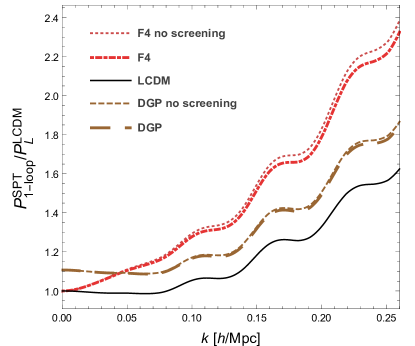
Figure 1: Ratio of 1-loop SPT to $\Lambda$CDM linear matter power spectra for $\Lambda$CDM, F4 and DGP models at redshift $z=0$ We fix cosmological parameters to the best fit of the WMAP Nine-year results [70].

In figure 1 we plot the ratios of the SPT 1-loop to linear matter power spectra, for models $\Lambda$CDM, F4 and the normal branch of DGP with crossover scale fixed by the Hubble constant, $r_{c}=H_{0}^{-1}$; in appendix A we give a brief summary of these models. We fix the cosmological parameters to $\Omega_{m}=0.281$, $\Omega_{b}=0.046$, $h=0.697$, $n_{s}=0.971$, and $\sigma_{8}=0.82$, corresponding to WMAP 9 years best fit to $\Lambda$CDM [70]. For F4 model, the background cosmology is indistinguishable to that in $\Lambda$CDM. This is not the case for DGP. However, as it is usual in the literature, for DGP we fix to a $\Lambda$CDM background. In such a way we can compare the differences in the growth of perturbations due to the fifth force and not to a different Hubble flow. Despite this, the power spectrum in DGP suffers a scale independent shift because $A(k,t)=A(t)\neq A_{0}$. We plot the power spectra with and without screenings; the latter are provided by setting $M_{2}=M_{3}=0$ in eq. (2.1). We stress out that for $\Lambda$CDM we make use of their exact kernels, that differ to those using EdS kernels by about 1% at quasi-linear scales. For the three models we use the same linear $\Lambda$CDM power spectrum as input, and thereafter we rescale it with

$$P_{L}(k,t)=\left(\frac{D_{+}(k,t)}{D_{+}^{\text{$\Lambda$CDM}}(t_{0})}\right)^{2}P_{L}^{\Lambda\text{CDM}}(k,t_{0}),$$ (2.46)

to get the linear power spectra in MG. This prescription is valid for models sharing an early EdS phase, as the majority of MG models considered in cosmology, and particularly to those used here. Otherwise, the linear power spectrum can be computed from an Einstein-Boltzmann code as MGCAMB [71, 72].

3 Lagrangian biased tracers in modified gravity

In large scale cosmological surveys, most of the objects of interest do not follow exactly the patterns of the underlying matter clustering, but their evolution is encoded in the statistics of tracers that provide biased estimations of matter statistics. Since we are interested in late time dynamics, where structure formation takes place, we assume all the matter is in the form of dark matter, and baryonic effects are not accounted for; instead all high nonlinearities are encapsulated into the bias parameters. In subsection 3.1, we apply the bias to initial, yet linear fields, which is the Lagrangian bias approach. Thereafter, nonlinear evolution takes place, which is studied in subsection 3.2.

3.1 Initially biased tracers

We filter the initial matter overdensities over a spatial scale $R_{\Lambda}$, that smooths out small scales, $q\lesssim R_{\Lambda}$ (or $k\gtrsim\Lambda=1/R_{\Lambda}$ in Fourier space), nonlinear fluctuations of the overdensity field as

$$\delta_{R}({\text{\bf q}})=\int d^{3}q^{\prime}W(|{\text{\bf q}}-{\text{\bf q}}^{\prime}|;R_{\Lambda})\delta_{m}({\text{\bf q}}^{\prime}),$$ (3.1)

and assume the existence of a function $F$ that relates the density fluctuations $\delta_{X}({\text{\bf q}})$ of tracers with a given set of operators constructed out of the fields that enter the theory. We consider smoothed overdensities of the underlying dark matter field, and the additional gravitational scalar field. Nevertheless, we may note from the Klein-Gordon equation that

$$\frac{k^{2}}{2a^{2}}\varphi=(A(k)-A_{0})\tilde{\delta}=2A_{0}\beta^{2}\frac{k^{2}\tilde{\delta}}{m^{2}a^{2}}+\mathcal{O}\left(\frac{k^{4}}{m^{4}a^{4}}\right),$$ (3.2)

where the first equality is valid at first order in field fluctuations and the second is obtained by expanding in powers of $k^{2}/m^{2}a^{2}$. Thus, the inclusion of bias expansion dependence on $\nabla^{2}\varphi$ is degenerated with a bias dependence on $\nabla^{2}\delta$, and equivalently a bias operator $\varphi$ is degenerated with an operator $\delta$. For that reason we will assume a Lagrangian bias function of the form

$$1+\delta_{X}({\text{\bf q}})=F(\delta_{R}({\text{\bf q}}),\nabla^{2}\delta_{R}({\text{\bf q}})).$$ (3.3)

We thus expect that our formalism accomodates better for $k$-modes smaller than the corresponding scalar field mass. A similar expansion to the one in eq. (3.2) can be performed to the growth equation of linear overdensities [eq. (2.4)]. Showing that at sufficently large scales we can effectively describe the effects of the fifth force, and the biasing in MG models with $m\neq 0$, with higher order derivative operators.

We now Fourier transform eq. (3.3) over both arguments to get

$$1+\delta_{X}({\text{\bf q}})=\int\frac{d^{2}\bf{\Lambda}}{(2\pi)^{2}}\tilde{F}({\bf\Lambda})e^{i{\bf D}\cdot{\bf\Lambda}},$$ (3.4)

with vectors $\mathbf{\Lambda}=(\lambda,\eta)$ and $\mathbf{D}=(\delta_{R},\nabla^{2}\delta_{R})$. We call to $\lambda$ and $\eta$ the spectral bias parameters corresponding to bias operators $\delta_{R}$ and $\nabla^{2}\delta_{R}$, respectively, and we define the bias parameters as [16, 12]

$$b_{nm}\equiv\int\frac{d^{2}\mathbf{\Lambda}}{(2\pi)^{2}}\tilde{F}(\mathbf{\Lambda})e^{-\frac{1}{2}\mathbf{\Lambda}^{\text{T}}\mathbf{\Sigma}\mathbf{\Lambda}}(i\lambda)^{n}(i\eta)^{m},$$ (3.5)

with a covariance matrix given by $\Sigma_{11}=\langle\delta_{R}^{2}\rangle=\sigma^{2}_{R}$, $\Sigma_{12}=\Sigma_{21}=\langle\delta_{R}\nabla^{2}\delta_{R}\rangle$, and $\Sigma_{22}=\langle(\nabla^{2}\delta_{R})^{2}\rangle$. We identify $b_{n0}$ with the local (in matter density) Lagrangian bias of order $n$, $b_{n0}=b_{n}$; while $b_{01}$ with the linear bias in the curvature, commonly written as $b_{01}=b_{\nabla^{2}}$. Nevertheless, we keep in mind that $b_{01}$ is introduced from an operator $\nabla^{2}\varphi$ which turns out, fortunately, to be degenerated with $\nabla^{2}\delta$.

The local $b_{n0}$ are already renormalized in the sense of ref. [8], i.e., the biased tracers statistics have no zero-lag correlators. But strictly, the $b_{nm}$ biases require further renormalization in order to remove subleading dependences on the smoothing kernel: For scales much larger than the smoothing $R_{\Lambda}$, tracers statistics should not depend on $R_{\Lambda}$, but the existence of the BAO bump in the correlation function at about $r_{\text{BAO}}\simeq 110\,\text{Mpc}/h$ with a width of $\Delta r_{\text{BAO}}\simeq 20\,\text{Mpc}/h$ makes the smoothing-independence condition more restrictive. If it is not accomplished, an artificial damping of the BAO peak is produced. This observation led to the introduction and renormalization of curvature and higher order derivative bias operators [10]. Under our bias definition, that renormalization is provided by replacing the factor $(i\eta)^{n}$ by $(i(\eta+W_{1}R_{\Lambda}^{2}\lambda))^{n}$ in eq. (3.5), where $W_{1}$ is the second term in the expansion of the filtering function in Fourier space, $\tilde{W}(kR_{\Lambda})=\sum_{n=0}^{\infty}W_{n}(kR_{\Lambda})^{2n}$ [12]. This reintroduction of the filtering kernel makes the results independent of the smoothing scale up to order $\mathcal{O}(R^{4}_{\Lambda}\nabla^{4}\delta_{R})$, that can be further improved by considering higher derivatives operators as arguments of the bias function $F$.

Leaving aside these complications, we can deal directly with the definition (3.5), and keep in mind that the renormalization procedure makes the statistics $R_{\Lambda}$ independent. For example, we can replace $\xi_{R}(q)=\langle\delta_{R}({\text{\bf q}}_{1})\delta_{R}({\text{\bf q}}_{2})\rangle$ by $\xi_{L}(q)=\langle\delta({\text{\bf q}}_{1})\delta({\text{\bf q}}_{2})\rangle$ as long as $q\gg R_{\Lambda}$, the other terms in the bias expansion will deal with the fact that $\xi_{R}=\xi_{L}+2W_{1}R_{\Lambda}^{2}\nabla^{2}\xi_{L}+\mathcal{O}(R_{\Lambda}^{4}\nabla^{4}\xi_{L})$.

Now, we come back to eq.(3.4) and multiply the integrand by $1=e^{-\frac{1}{2}\mathbf{\Lambda}^{\text{T}}\mathbf{\Sigma}\mathbf{\Lambda}}e^{\frac{1}{2}\mathbf{\Lambda}^{\text{T}}\mathbf{\Sigma}\mathbf{\Lambda}}$. We then expand $e^{\frac{1}{2}\mathbf{\Lambda}^{\text{T}}\mathbf{\Sigma}\mathbf{\Lambda}+i{\bf\Lambda}\cdot{\bf D}}$ in powers of $\lambda$ and $\eta$, and with the use of eq. (3.5) we obtain the tracer overdensity

$$\delta_{X}({\text{\bf q}})=b_{10}\delta+b_{01}\nabla^{2}\delta+\frac{1}{2}b_{20}\delta^{2}+b_{11}\delta\nabla^{2}\delta+\frac{1}{2}b_{02}(\nabla^{2}\delta)^{2}+\cdots,$$ (3.6)

up to second order. Given our discussion above, we have omitted to write the label $R$ in the matter fluctuations and assume this equation is valid for $q\gg R_{\Lambda}$. The linear correlation function is given by $\xi_{X,L}=\langle\delta_{X}({\text{\bf q}}^{\prime}+{\text{\bf q}})\delta_{X}({\text{\bf q}}^{\prime})\rangle$, or

$$\xi_{X}(q)=b_{10}^{2}\xi_{L}(q)+2b_{10}b_{01}\nabla^{2}\xi_{L}(q)+b_{01}^{2}\nabla^{4}\xi_{L}(q),$$ (3.7)

since

$$\nabla^{2}\xi_{L}(q) =\langle\delta({\text{\bf q}}^{\prime})\nabla^{2}\delta({\text{\bf q}}^{\prime}+{\text{\bf q}})\rangle=-\int\frac{d^{3}k}{(2\pi)^{3}}e^{i{\text{\bf k}}\cdot{\text{\bf q}}}k^{2}P_{L}(k),$$ (3.8)

$$\nabla^{4}\xi_{L}(q) =\langle\nabla^{2}\delta({\text{\bf q}}^{\prime})\nabla^{2}\delta({\text{\bf q}}^{\prime}+{\text{\bf q}})\rangle=\int\frac{d^{3}k}{(2\pi)^{3}}e^{i{\text{\bf k}}\cdot{\text{\bf q}}}k^{4}P_{L}(k).$$ (3.9)

The Fourier transform gives the linear power spectrum for tracers

$$P_{X,L}(k)=(b_{10}-b_{01}k^{2})^{2}P_{L}(k),$$ (3.10)

which has the same form as the peak model (PM) linear bias with

$$b_{10}=b_{10}^{\text{PM}},\qquad b_{01}=-b_{01}^{\text{PM}}.$$ (3.11)

We notice that the notation $b_{nm}$ for bias is adopted also in the context of non-Gaussian linear fields [74], and is not related with our notation.

We have not assumed the time at which the initial fields are defined, and therefore the linear statistics we derived apply equally well to the case of Eulerian biased tracers. If fields are evolved nonlinearly, Eulerian and Lagrangian biasing schemes give different results.

3.2 Evolution of biased tracers in PT

As is common practice, we make the assumption that the number of tracers is conserved,

$$(1+\delta_{X}({\text{\bf x}}))d^{3}x=(1+\delta_{X}({\text{\bf q}}))d^{3}q,$$ (3.12)

that is clearly a simplification since tracers can merge or be created. Developing this equation, we obtain

$$1+\delta_{X}({\text{\bf x}}) =\int d^{3}q\,\delta_{\text{D}}({\text{\bf x}}-{\text{\bf q}}-\mathbf{\Psi})(1+\delta_{X}({\text{\bf q}}))$$

$$=\int\frac{d^{3}k}{(2\pi)^{3}}\int d^{3}qe^{i{\text{\bf k}}\cdot({\text{\bf x}}-{\text{\bf q}}-\mathbf{\Psi})}\int\frac{d^{2}\mathbf{\Lambda}}{(2\pi)^{2}}\tilde{F}(\mathbf{\Lambda})e^{i\mathbf{\Lambda}\cdot\mathbf{D}},$$ (3.13)

where in the second equality we used eq. (3.4).

We notice that the Lagrangian displacement entering eq. (3.2) is that of dark matter and not that of tracers. On top of that, the biasing is applied by using eq. (3.3). However, tracers are subject to tidal forces not experienced by dark matter particles, inducing a velocity bias. Indeed, it is known that this bias should enter in the description as a higher derivative operator, on the same footing as the operator $\nabla^{2}\delta$ [18, 73]. In peaks theory this bias is completely determined once the linear power spectrum is given and a filtering kernel is chosen [75, 76], and shifts the Lagrangian displacement field by a term $\propto k^{2}\Psi(\mathbf{k})$. Having this in mind, we can think of considering a bias operator $\nabla\cdot\nabla^{2}\mathbf{\Psi}$ with bias parameter $b_{X,\Psi}$ as an argument of $F$. We note however that at leading order in PT it becomes degenerated with the density Laplacian bias operator because $\nabla\cdot\mathbf{\Psi}^{(1)}=-\delta_{L}$. Hence, the effect of the velocity bias, introduced here through the Lagrangian displacement, is to shift the bias parameter $b_{01}$ to $b_{01}-b_{\Psi,X}$. This impact of a linear velocity bias over the biased overdensities is consistent with known results in the, more common, Eulerian approach and in the Lagrangian peaks formalism; see [73, 77, 76] and sects. 2.7 and 6.9 of [18].

Now, the LPT tracers power spectrum is given by [33, 16, 12]

$$(2\pi)^{3}\delta_{\text{D}}({\text{\bf k}})+P_{X}^{\text{LPT}}(k)=\int d^{3}qe^{i{\text{\bf k}}\cdot{\text{\bf q}}}\int\frac{d^{2}\mathbf{\Lambda}_{1}}{(2\pi)^{2}}\frac{d^{2}\mathbf{\Lambda}_{2}}{(2\pi)^{2}}\tilde{F}(\mathbf{\Lambda}_{1})\tilde{F}(\mathbf{\Lambda}_{2})\langle e^{i[\mathbf{\Lambda}_{1}\cdot\mathbf{D}_{1}+\mathbf{\Lambda}_{2}\cdot\mathbf{D}_{2}+{\text{\bf k}}\cdot\Delta]}\rangle,$$ (3.14)

where $\mathbf{D}_{1,2}=(\delta_{R}({\text{\bf q}}_{1,2}),\nabla^{2}\delta_{R}({\text{\bf q}}_{1,2}))$ and

$$\Delta_{i}=\Psi_{i}(q_{2})-\Psi_{i}(q_{1}) =\int\frac{d^{3}k}{(2\pi)^{3}}(e^{i{\text{\bf k}}\cdot{\text{\bf q}}_{2}}-e^{i{\text{\bf k}}\cdot{\text{\bf q}}_{1}})\Psi_{i}({\text{\bf k}})$$

$$=\sum_{n=1}^{\infty}\int\frac{d^{3}k}{(2\pi)^{3}}(e^{i{\text{\bf k}}\cdot{\text{\bf q}}_{2}}-e^{i{\text{\bf k}}\cdot{\text{\bf q}}_{1}})\Psi_{i}^{(n)}({\text{\bf k}})$$ (3.15)

is the difference of Lagrangian displacement fields separated by a distance ${\text{\bf q}}={\text{\bf q}}_{2}-{\text{\bf q}}_{1}$. We will employ the cumulant expansion theorem

$$\langle e^{iX}\rangle=\exp\left(\sum_{N=1}^{\infty}\frac{i^{N}}{N!}\langle X^{N}\rangle_{c}\right)=\exp\left(-\frac{1}{2}\langle X^{2}\rangle_{c}-\frac{i}{6}\langle X^{3}\rangle_{c}+\cdots\right),$$ (3.16)

where $\langle X^{N}\rangle_{c}$ denotes the cumulant of $X^{N}$. In this case we have $X=\mathbf{\Lambda}_{1}\cdot\mathbf{D}_{1}+\mathbf{\Lambda}_{2}\cdot\mathbf{D}_{2}+{\text{\bf k}}\cdot\Delta$.

The strategy now is to expand all terms that contain bias spectral parameters $\lambda$ and $\eta$ with the exception of a term $e^{-\frac{1}{2}\mathbf{\Lambda}^{\text{T}}\mathbf{\Sigma}\mathbf{\Lambda}}$, and use the definition of eq. (3.5) to obtain the biases. Keeping the local bias up to second order and the curvature bias to first order we obtain

$$(2\pi)^{3}\delta_{\text{D}}({\text{\bf k}}) +P_{X}^{\text{LPT}}(k)=\int d^{3}qe^{i{\text{\bf k}}\cdot{\text{\bf q}}}e^{-\frac{1}{2}k_{i}k_{j}A_{ij}-\frac{i}{6}k_{i}k_{j}k_{k}W_{ijk}}\Bigg{[}1+b_{10}^{2}\xi_{L}+2ib_{10}k_{i}U_{i}+\frac{1}{2}b_{20}^{2}\xi_{L}^{2}$$

$$-(b_{20}+b_{10}^{2})k_{i}k_{j}U_{i}U_{j}+2ib_{10}b_{20}\xi_{L}k_{i}U_{i}+ib_{10}^{2}k_{i}U_{i}^{11}+ib_{20}k_{i}U_{i}^{20}-b_{10}k_{i}k_{j}A_{ij}^{10}$$

$$+2b_{10}b_{01}\nabla^{2}\xi_{L}-2ib_{01}k_{i}\nabla_{i}\xi_{L}+b_{01}^{2}\nabla^{4}\xi_{L}\Bigg{]},$$ (3.17)

with functions [35]

$$U^{mn}_{i}({\text{\bf q}}) =\langle\delta^{m}_{L}({\text{\bf q}}_{1})\delta^{n}_{L}({\text{\bf q}}_{2})\Delta_{i}\rangle_{c},$$ (3.18)

$$A_{ij}^{mn}({\text{\bf q}}) =\langle\delta^{m}_{L}({\text{\bf q}}_{1})\delta^{n}_{L}({\text{\bf q}}_{2})\Delta_{i}\Delta_{j}\rangle_{c},$$ (3.19)

$$W_{ijk}({\text{\bf q}}) =\langle\Delta_{i}\Delta_{j}\Delta_{k}\rangle_{c},$$ (3.20)

and $U_{i}=U^{10}_{i}$, $A_{ij}=A_{ij}^{00}$. In appendix C.2 we find the explicit expressions for these q-functions in generalized cosmologies. The complete expansion that includes second order curvature bias can be found in [12]; the terms we are neglecting here are subdominant. One can continue this process to include higher order biases, but this necessarily needs the introduction of higher order fluctuations.

If we keep all terms quadratic in $k$ in the exponential of eq. (3.2) and expand the rest, we can Fourier transform it and, by performing several multivariate Gaussian integrations, obtain an analytical expression for the correlation function. This is the approach of CLPT, first developed in [35]. But, in order to treat on an equal footing linear and nonlinear fields contributions, in this work we keep exponentiated only the linear piece of $A_{ij}$ and expand the rest, as was done in [78], obtaining the CLPT correlation function for tracers,

$$1+\xi_{X}^{\text{CLPT}}(r) =1+\xi^{\text{CLPT}}(r)+b_{10}\text{x}_{10}(r)+b_{10}^{2}\text{x}_{20}(r)+b_{20}\text{x}_{01}(r)+b_{10}b_{20}\text{x}_{11}(r)$$

$$\quad+b_{01}^{2}\text{x}_{02}(r)+2(1+b_{10})b_{01}\text{x}_{\nabla^{2}}(r)+b_{01}^{2}\text{x}_{\nabla^{4}}(r),$$ (3.21)

with matter correlation function

$$1+\xi^{\text{CLPT}}(r) =\int\frac{d^{3}q}{(2\pi)^{3/2}|\mathbf{A}_{L}|^{1/2}}e^{-\frac{1}{2}({\text{\bf r}}-{\text{\bf q}})^{\mathbf{T}}\mathbf{A}_{L}^{-1}({\text{\bf r}}-{\text{\bf q}})}\Bigg{(}1-\frac{1}{2}A_{ij}^{loop}G_{ij}+\frac{1}{6}\Gamma_{ijk}W_{ijk}\Bigg{)},$$ (3.22)

where $g_{i}=(A_{L}^{-1})_{ij}(q_{j}-r_{j})$, $G_{ij}=(A_{L}^{-1})_{ij}-g_{i}g_{j}$, and $\Gamma_{ijk}=(A_{L}^{-1})_{\{ij}g_{k\}}+g_{i}g_{j}g_{k}$. The “1” in between the parentheses corresponds to the Zel’dovich approximation. The notation $\text{x}_{\text{NM}}$ (and for the $\text{a}_{\text{NM}}$ introduced below) means that these bias contributions are multiplied by the linear local bias to the N power times the second order local bias to the M power. These functions are

$$\text{x}_{10}(r) =\int\frac{d^{3}q}{(2\pi)^{3/2}|\mathbf{A}_{L}|^{1/2}}e^{-\frac{1}{2}({\text{\bf r}}-{\text{\bf q}})^{\mathbf{T}}\mathbf{A}_{L}^{-1}({\text{\bf r}}-{\text{\bf q}})}(-2U_{i}g_{i}-A^{10}_{ij}G_{ij}),$$ (3.23)

$$\text{x}_{20}(r) =\int\frac{d^{3}q}{(2\pi)^{3/2}|\mathbf{A}_{L}|^{1/2}}e^{-\frac{1}{2}({\text{\bf r}}-{\text{\bf q}})^{\mathbf{T}}\mathbf{A}_{L}^{-1}({\text{\bf r}}-{\text{\bf q}})}(\xi_{L}-U_{i}U_{j}G_{ij}-U_{i}^{11}g_{i}),$$ (3.24)

$$\text{x}_{01}(r) =\int\frac{d^{3}q}{(2\pi)^{3/2}|\mathbf{A}_{L}|^{1/2}}e^{-\frac{1}{2}({\text{\bf r}}-{\text{\bf q}})^{\mathbf{T}}\mathbf{A}_{L}^{-1}({\text{\bf r}}-{\text{\bf q}})}(-U_{i}^{20}g_{i}-U_{i}U_{j}G_{ij}),$$ (3.25)

$$\text{x}_{11}(r) =\int\frac{d^{3}q}{(2\pi)^{3/2}|\mathbf{A}_{L}|^{1/2}}e^{-\frac{1}{2}({\text{\bf r}}-{\text{\bf q}})^{\mathbf{T}}\mathbf{A}_{L}^{-1}({\text{\bf r}}-{\text{\bf q}})}(-2\xi_{L}U_{i}g_{i}),$$ (3.26)

$$\text{x}_{02}(r) =\int\frac{d^{3}q}{(2\pi)^{3/2}|\mathbf{A}_{L}|^{1/2}}e^{-\frac{1}{2}({\text{\bf r}}-{\text{\bf q}})^{\mathbf{T}}\mathbf{A}_{L}^{-1}({\text{\bf r}}-{\text{\bf q}})}\frac{1}{2}\xi_{L}^{2},$$ (3.27)

$$\text{x}_{\nabla^{2}}(r) =\int\frac{d^{3}q}{(2\pi)^{3/2}|\mathbf{A}_{L}|^{1/2}}e^{-\frac{1}{2}({\text{\bf r}}-{\text{\bf q}})^{\mathbf{T}}\mathbf{A}_{L}^{-1}({\text{\bf r}}-{\text{\bf q}})}\nabla^{2}\xi_{L}(q),$$ (3.28)

$$\text{x}_{\nabla^{4}}(r) =\int\frac{d^{3}q}{(2\pi)^{3/2}|\mathbf{A}_{L}|^{1/2}}e^{-\frac{1}{2}({\text{\bf r}}-{\text{\bf q}})^{\mathbf{T}}\mathbf{A}_{L}^{-1}({\text{\bf r}}-{\text{\bf q}})}\nabla^{4}\xi_{L}(q).$$ (3.29)

The explicit computation that leads to eq. (3.2), yields also a term $\nabla_{i}\xi_{L}(q)g_{i}$. However, as noted in [60], this is highly degenerated with $\nabla^{2}\xi_{L}(q)$: indeed, both terms correspond to a contribution $-k^{2}P_{L}$ to the SPT power spectrum. Therefore, we have substituted the combination $2b_{10}b_{01}\nabla^{2}\xi_{L}(q)+2b_{01}\nabla_{i}\xi_{L}(q)g_{i}$ by $2(1+b_{10})b_{01}\nabla^{2}\xi_{L}(q)$ when writing eq. (3.2).

LPT describes quite well the BAO wiggles in the power spectrum, but it fails to follow its broadband trend. Since here we are interested in the latter also, we expand all terms out of the exponential in eq. (3.2) and perform the q integration to obtain the SPT power spectrum for Lagrangian biased tracers. This procedure involves lengthy mathematical manipulations that are presented in appendix D, yielding

$$P^{\text{SPT}}_{X}(k) =P_{L}(k)+P_{22}(k)+P_{13}(k)+b_{10}\text{a}_{10}(k)+b_{20}\text{a}_{01}(k)+b_{10}^{2}\text{a}_{20}(k)$$

$$\quad+b_{10}b_{20}\text{a}_{11}(k)+b_{20}^{2}\text{a}_{02}(k)-2(1+b_{10})b_{01}k^{2}P_{L}(k)+b_{01}^{2}k^{4}P_{L}(k)$$ (3.30)

with $P_{22}$ and $P_{13}$ given by eqs. (2.43, 2.44), and

$$\text{a}_{10}(k) =2P_{L}(k)+\frac{10}{21}R_{1}(k)+\frac{6}{7}R_{1+2}(k)+\frac{6}{7}R_{2}(k)+\frac{6}{7}Q_{5}(k)+2Q_{7}(k)-2\sigma^{2}_{L}k^{2}P_{L}(k),$$ (3.31)

$$\text{a}_{01}(k) =Q_{9}(k)+\frac{3}{7}Q_{8}(k),$$ (3.32)

$$\text{a}_{20}(k) =P_{L}(k)+\frac{6}{7}R_{1+2}(k)+Q_{9}(k)+Q_{11}(k)-\sigma^{2}_{L}k^{2}P_{L}(k),$$ (3.33)

$$\text{a}_{11}(k) =2Q_{12}(k),$$ (3.34)

$$\text{a}_{02}(k) =\frac{1}{2}Q_{13}(k),$$ (3.35)

where $Q$ and $R$ functions are given in appendix C.1. It is worth to pointing out that the results of Sect. 2.2 are allowing us to identify eq. (3.2) with the SPT power spectrum with Lagrangian biased tracers in generalized cosmologies. We further notice that its structure is similar to that of [16]; but in MG the $Q$ and $R$ functions are different. Also, here we find a function $R_{1+2}$, which for EdS coincides with the combination $R_{1}+R_{2}$.

3.3 Numerical results

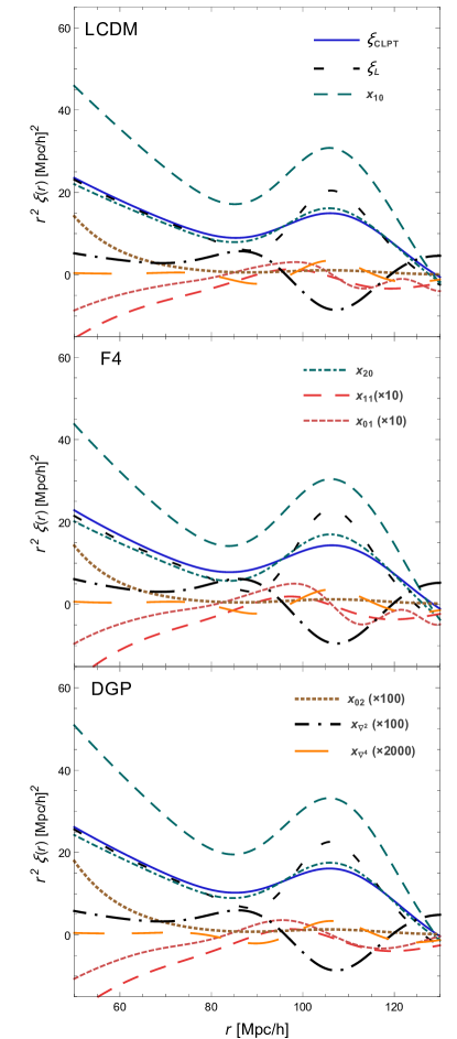
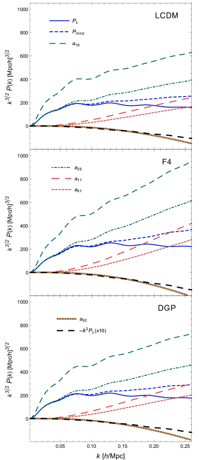
Figure 2: Bias components for the CLPT correlation function [eq. (3.2)] and SPT power spectrum [eq. (3.2)] for models $\Lambda$CDM model, F4 and the normal branch of DGP with crossover scale $r_{c}=1/H_{0}$. We fix cosmological parameters to the best fit of the WMAP Nine-year results [70] and evaluate at redshift $z=0$.

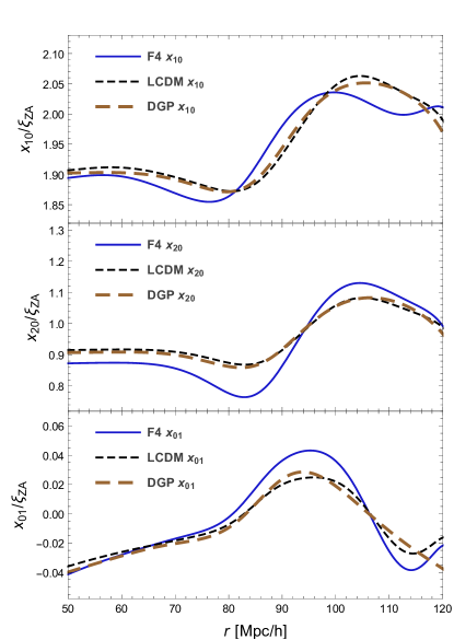
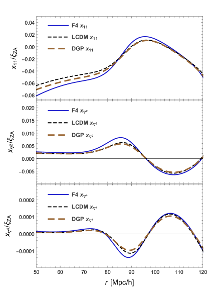
Figure 3: Ratios of bias functions $\text{x}_{\text{MN}}$ over the Zel’dovich approximation correlation function.

To compute the SPT power spectrum and the CLPT correlation function we have developed the code MGPT that we make public available with this article. First, it calculates the set of $Q$ and $R$ functions in appendix C.1, for which the angular $x$ integration uses a Gauss-Legendre quadrature and the radial part uses the trapezoidal quadrature. At each step of the integration we solve the differential equations eqs. (2.20, 2.21) to obtain the functions $D_{\mathcal{A}}$, $D_{\mathcal{B}}$ using the solver bsstep [79], as well as the corresponding third order growth functions. The “time” variable is chosen as $\eta=\ln a$, with $a$ the scale factor, starting with EdS initial conditions at $\eta_{ini}=-6$. Thereafter, the code computes the $q$-functions of appendix C.2 and the CLPT contributions of eqs. (3.22-3.29).

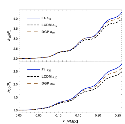
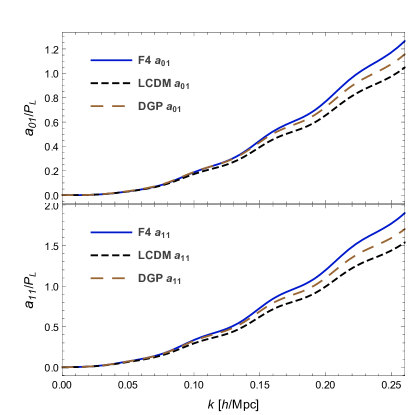
Figure 4: Ratios of bias functions $\text{a}_{\text{MN}}$ over the linear power spectrum.

In figure 2 we show the different contributions $a_{\text{NM}}$ and $\text{x}_{\text{NM}}$ to the tracers power spectrum and correlation function for models $\Lambda$CDM, F4 and the normal branch of DGP with crossover scale $r_{c}=1/H_{0}$. Though these specific models are already ruled out by observations, they show the kind of growth of fluctuations expected in MG theories. As in section 2.2, in the $\Lambda$CDM case we make use of their exact kernels.

In figure 3 we plot the ratios of the $\text{x}_{\text{NM}}$ bias contributions to the Zel’dovich approximation correlation function for each model; while in figure 4 we plot the ratios of the $\text{a}_{\text{NM}}$ bias contributions to the linear power spectrum for each model.

4 Simple model for halo bias in $f(R)$ gravity

So far, we were concerned in how the bias parameters appear in the structure of LPT and SPT statistics, saying nothing about their own evolution. In this section we put forward a model for the estimation of local bias in MG, which although is not rigorous, reflects the following observation: Generally MG is scale dependent and because the fifth force is attractive (in general), matter fluctuations grow faster than in GR. This implies that the critical density for collapse $\delta_{c}$ is smaller in MG. On the other hand, by the same reason the power spectrum acquires more strength and the variance

$$S(R)\equiv\sigma^{2}_{R}=\int\frac{d^{3}k}{(2\pi)^{3}}|\tilde{W}(kR)|^{2}P_{L}(k)$$ (4.1)

becomes larger in MG than in GR. Typically, a local bias depends on the critical density for collapse $\delta_{c}$ and on the fluctuations variance, schematically $b_{n}\sim\left(\frac{\delta_{c}}{\sigma_{R}^{2}}\right)^{n}+\cdots$, which is a good approximation for massive halos. This implies that

$$b_{n}^{\text{MG}}<b_{n}^{\text{GR}},$$ (4.2)

reflecting that halos are more efficiently formed in MG than in GR. This effect has been observed recently in N-body simulations [57]. The rest of this section is aimed to show this property in $f(R)$ theories.

4.1 Bias model

There are some obstacles when describing bias in generalized cosmologies. First, the scale dependence of growth functions implies that even linear bias is scale dependent; second, Birkhoff’s theorem is not valid, and therefore cannot be applied to spherical collapse calculations or to the peak-background split (PBS) prescription. From the work of [19] we know that the Lagrangian linear local bias evolves as $b_{1}(z)\propto D^{-1}_{+}(k,z)$. Bearing this in mind, perhaps the most easy way to get a model for bias parameters is to compute it from a universal mass function at sufficiently large redshift $z_{i}$ at which the evolution is indistinguishable from GR (as is the case for the models we have used to show our results), and the peak background split procedure is valid. In such a way we obtain a bias for GR as a function of mass $b(R(M),t_{ini})$ and thereafter we evolve it with a growth function that we choose as

$$\tilde{D}_{+}^{\text{MG}}(M,z;z_{i})\equiv\frac{\sigma_{R,\text{MG}}(M,z)}{\sigma_{R,\text{MG}}(M,z_{i})}=\frac{\sigma_{R,\text{MG}}(M,z)}{\sigma_{R,\text{$\Lambda$CDM}}(M,z)}D_{+}^{\text{$\Lambda$CDM}}(z;z_{i})$$ (4.3)

where $M$ is the mass enclosed by the spherical perturbation and $R=(3M/4\pi\bar{\rho}_{m}(z=0))^{1/3}$ its Lagrangian radius. The only requirement we adopt is that at the initial redshift $z_{i}$, the evolution of fluctuations in MG and GR are the same for all scales of interest.

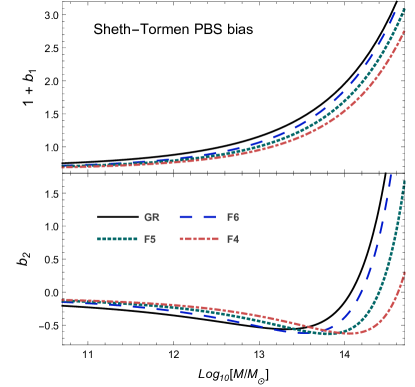
Figure 5: Analytical large scale bias $b_{LS}=1+b_{1}$ and bias $b_{2}$ for models $\Lambda$CDM, F6, F5 and F4. We use eqs. (4.8, 4.9) with Sheth-Tormen parameters $q=0.707$ and $p=0.3$. The filtering function is a top-hat of width given by the Lagrangian radius $R(M)$.

We consider a mass function that gives the number density of halos over a mass interval $(M,M+dM)$,

$$n(M,z)=\frac{\bar{\rho}}{M^{2}}\nu f(\nu)\left|\frac{d\log\nu}{d\log M}\right|,$$ (4.4)

with $\nu f(\nu)$ the multiplicity function and $\nu=\delta_{c}/\sigma_{R}$ is the peak significance threshold. We apply the PBS prescription to obtain the local biases at redshift $z_{i}$

$$b_{n}(M,z_{i}) =\frac{(-1)^{n}}{\sigma^{n}_{R}(M,z_{i})}\frac{1}{\nu_{i}f(\nu_{i})}\frac{d^{n}\nu_{i}f(\nu_{i})}{d\nu_{i}^{n}},$$ (4.5)

and thereafter we evolve them to redshift $z$ with the growth of eq. (4.3) as

$$b_{n}(M,z) =\frac{1}{[\tilde{D}_{+}^{\text{MG}}(M,z;z_{i})]^{n}}b_{n}(M,z_{i})=\frac{(-1)^{n}}{\sigma^{n}_{R}(M,z)}\frac{1}{\nu_{i}f(\nu_{i})}\frac{d^{n}\nu_{i}f(\nu_{i})}{d\nu_{i}^{n}},$$ (4.6)

with $\nu_{i}=\nu(z_{i})$. It is necessary to specify the time of evaluation of the peak significance because unlike in GR, it is time dependent in MG. We emphasize that the bias parameters obtained from the PBS prescription coincide with those defined in eq. (3.5), as it was shown in [12].

In $\Lambda$CDM the density collapse threshold $\delta_{c}^{\text{GR}}$ is scale independent and weakly depends on the cosmology. Instead, in MG it becomes scale dependent and also dependent on the environmental density $\delta_{env}$ because of violation of Birkhoff’s theorem. It is possible to obtain a unique function $\delta_{c}^{\text{MG}}(M,z)$ by averaging over environmental overdensities or by choosing an specific one out of a known distribution of environments [80]. An alternative route is adopted in [81], where that average is performed to the initial conditions using Gaussian peaks model [82]; that work also provides a fitting function for the top-hat density collapse threshold in $f(R)$ gravity, that we will use also here to exemplify our bias model.

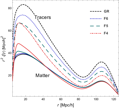
Figure 6: Correlation function for tracers (non-solid curvers) using first and second order biases from the results of figure 5, with the halo masses fixed to $10^{13.5}M_{\odot}$. The lower, solid curves, show the correlation functions for matter. We plot the models $\Lambda$CDM (black), F6 (blue), F5 (green) and F4 (red).

The multiplicity function may be parametrized as [6]

$$\nu f(\nu)=\mathcal{N}\sqrt{\frac{2}{\pi}q\nu^{2}}(1+(q\nu^{2})^{-p})e^{-q\nu^{2}/2},$$ (4.7)

where the number $\mathcal{N}$ normalizes the multiplicity as $\int_{0}^{\infty}d\nu f(\nu)=1/2$. The two free parameters take values $q=1$ and $p=0$ for Press-Schechter [7], and $q=0.707$ and $p=0.3$ for Sheth-Tormen [6] mass functions. The linear and second order local biases become

$$b_{1}(M) =\frac{1}{\tilde{D}_{+}}\frac{1}{\delta_{c}}\left(q\nu^{2}-1+\frac{2p}{1+(q\nu^{2})^{p}}\right),$$ (4.8)

$$b_{2}(M) =\frac{1}{\tilde{D}_{+}^{2}}\frac{1}{\delta_{c}^{2}}\left(q^{2}\nu^{4}-3q\nu^{2}+\frac{2p(2q\nu^{2}+2p-1)}{1+(q\nu^{2})^{p}}\right).$$ (4.9)

It has been shown that the Sheth-Tormen model gives good results for the halo mass function also in $f(R)$ gravity [83]. Motivated by this, we compute our analytical formula for biases of eqs. (4.8-4.9) fed with the Sheth-Tormen mass function parameters and using a top-hat filter in the variance. We plot the cases $b_{1}$ and $b_{2}$ in figure 5 for GR, F6, F5 and F4 models. From here we strenghten our heuristic result in eq. (4.2). In the next subsection we compare our bias model to results obtained from excursion set theory.

Figure 6 shows the CLPT correlation functions for matter and for tracers with a fixed halo mass of $10^{13.5}M_{\odot}$, computed with the biases $b_{1}$ and $b_{2}$ shown in figure 5 and using eq. (3.2). This shows that regardless the MG model, the matter correlation functions are quite similar at large, linear scales, while for tracers they can differ significatively.

4.2 Excursion sets

Excursion set theory [84] identifies the places where virialized structures will form with overdensities that, when smoothed over that same region, exceed some critical value, that we take to be the top-hat density collapse $\delta_{c}$. Letting the smoothing lenght vary from $\infty$ to $R$ makes $\delta_{R}({\text{\bf q}})$ to describe a random walk with $R$ as the evolution variable, although it is convenient to parametrize the trajectories in terms of the variance $S(R)$ which decrease with $R$.

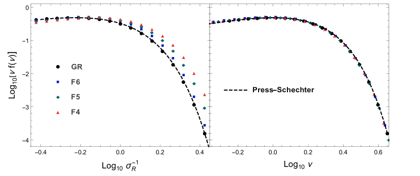
Figure 7: Multiplicity function $\nu f(\nu)$ as a function of $\log\sigma^{-1}_{R}$ (left panel), and as function of $\nu$ (right panel). We notice that while $\sigma_{R}$ is the same for all models, the peak significance $\nu$ is a model dependent quantity. The dashed curve shows the Press-Schechter analytical mass function. We have used the redshift for collapse $z_{c}=0$.

The different realizations of the overdensity produce an ensemble of walkers which cross the barrier $\delta^{\text{MG}}_{c}(M,z)$ at different “times” $S$. The main assumption in excursion set theory is that the halo mass function is directly related to the fraction $f_{\text{FU}}(S)dS$ of walkers that have their first (up-)crossing in the interval $(S,S+dS)$,

$$n(M,z)dM=\frac{\bar{\rho}}{M^{2}}f_{\text{FU}}(S)dS,$$ (4.10)

that when comparing to eq. (4.4) gives

$$f(\nu)d\nu=f_{\text{FU}}(S)dS\,,$$ (4.11)

which can be used to compute the bias parameters (4.6).

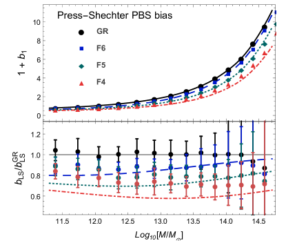
Figure 8: Large scales bias $b_{\text{LS}}=1+b_{1}$ for models $\Lambda$CDM, F6, F5 and F4 as a function of halo mass $M$. The analytical results make use of eq. (4.8) with $p=0$ and $q=1$ corresponding to Press-Schechter PBS bias in GR, and use the threshold density for collapse computed from the fitting functions provided in ref. [81]. We plot solid black curves for $\Lambda$CDM model, dashed blue for F6, dotted green for F5, and dotted-dashed for F4. The dots are the numerical results using excursion sets in section 4.2. The lower paner shows the ratio of these quantities to the analytical $\Lambda$CDM bias.

In order to estimate $f_{\text{FU}}$ we perform Monte Carlo simulations considering the simplest case of a sharp-$k$ filtering $\tilde{W}=\Theta_{H}(1/R(M)-k)$. In such a way the trajectories $\delta_{R}(S)$ are Markovian, meaning that each jump $\Delta\delta_{R}$ from $S$ to $S+\Delta S$ is uncorrelated with the previous ones, and are drawn from a Gaussian distribution. In $\Lambda$CDM this process can be solved analytically to obtain the Press-Schechter mass function and corresponding bias parameters. This is not the case for moving barriers, as those present in MG, and the solution should be found numerically. We emphasize that we are considering this procedure at initial time with an already environmental independent density collapse, so our approach is that of [81], but here we restrict our attention to the simplest case — the authors of that work consider subsequent refinenemts by accounting for top-hat window function, which has been discussed to be more proper [84], as well as drifting and diffusing barriers to model non-spherical collapse. Other approaches make this analysis for environmental dependent collapse densities and then average the resulting first up-crossing distributions [80, 85, 86, 83, 87].

We plot our results in figure 7, showing the multiplicity function as a function of $\log\sigma^{-1}_{R}$ in the left panel and as a function of $\nu$ in the right panel. Since we are taking the walkers at initial time, the variance, and hence $\sigma^{-1}_{R}$ is equal to all models. But this is not the case for $\nu=\delta_{c}/\sigma$ which is model dependent. We note that for the latter case, all the multiplicity functions are (almost) equal, suggesting a universal pattern. When properly rescaled to $\sigma^{-1}_{R}$, they look different. In ref. [81] (their figure 9), the authors present similar results to our plot in the left panel of figure 7.

The local linear bias is computed by taking the logarithmic derivative of $\nu f(\nu)$ and dividing by the collapse threshold $\delta_{c}$. In figure 8 the marks show our numerical results with error bars denoting the scattering after performing several runs for walkers. Together, we plot the analytical results obtained from eq. (4.8) using Press-Schechter parameters. For massive halos we find a decent agreement between our bias analytical formula and the numerics. For small masses our model underestimate the bias, though it follows correctly the trend of the data, as shown in the upper panel of figure 8.

5 Conclusions

In this work we have continued the development of perturbation theory for MG theories within the Lagrangian formalism. Our main goal was to develop a theory of large-scale-structure bias for MG models that was lacking in the literature. However, to develop the theory it was first necessary to understand the SPT power spectrum computed from the LPT formalism developed in a previous work [52]. In order to compute the SPT power spectrum, we found relations that connect the Lagrangian and Eulerian kernels to arbitrary order in PT and that holds for general cosmological models, these are given by eqs. (2.32) and (B). Using these kernels, our result for the SPT power spectrum is given by eqs. (2.43, 2.44) that exactly coincides with the expression valid for the $\Lambda$CDM model. Of course, in eqs. (2.43, 2.44) one should employ the $P_{L}$, $Q$- and $R$-functions corresponding to the appropriate cosmology. This derivation was in fact not known, although it was perhaps expected and, in any case, necessary for us to develop bias contributions. In Ref. [52] two of us have named the SPT power spectrum computed from eqs. (2.43, 2.44) as SPT*; now, we have demonstrated this result coincides with the SPT standard result.

To finally develop the bias theory for MG cosmological models, we start from Lagrangian, initially biased tracers. We consider smoothed overdensities of the underlying dark matter field and of the MG-related scalar field, and note that given the form of the Klein Gordon equation, the inclusion of bias expansion dependence on $\nabla^{2}\varphi$ is degenerated with a bias dependence on $\nabla^{2}\delta$. For that reason we assume a Lagrangian bias function with operators $\delta$ and $\nabla^{2}\delta$ as arguments that will finally conduct us to define the bias parameters $b_{nm}$ and explain the way to renormalize them with the prescription given in [12]. Then we computed the linear correlation function and power spectrum for biased tracers. Next step is to construct the full LPT power spectrum and the CLPT correlation function for biased tracers in alternative cosmologies with screening mechanisms, in which we introduced local bias to second order and curvature bias to first order to match consistency in the 1-loop approximation order. By doing this we have generalized, beyond $\Lambda$CDM, the $Q$ and $R$ functions which are building blocks of matter and tracers statistics; in appendix D we provide with all these functions.

In order to facilitate the use of our formalism, that implies the manipulation of many cumbersome formulae, we are making public available a new code, called MGPT (Modified Gravity Perturbation Theory), that computes all the necessary functions and the SPT power spectrum and the CLPT correlation function for $\Lambda$CDM and MG models that can be brought to a scalar-tensor description, e.g. through field redefinitions; the code is released in the github repository cosmoinin/MGPT. To illustrate the functionality and tests of code, we have computed these 2-point, 1-loop statistics for models $\Lambda$CDM, Hu-Sawicki $f(R)$ and DGP braneworld.

Finally, we put forward a simple halo bias model to illustrate its effects stemming from modifications of gravity. We note that in general terms the MG dynamics are scale dependent and because the fifth force is attractive (in many models), matter fluctuations grow faster than in GR, leading to a more efficient relaxation of bias, and implying that in general one can expect $b_{n}^{\text{MG}}<b_{n}^{\text{GR}}$. This result is generic and can contribute to distinguish MG models from $\Lambda$CDM. To illustrate this fact, we constructed a particular bias model for the Hu-Sawicki $f(R)$ gravity and compare our analytical results with excursion set theory. Our results are consistent and shown in figure 8, confirming that $b_{n}^{f(R)}<b_{n}^{\text{GR}}$ holds over a wide range of halo masses.

Appendix A MG models

This appendix aims to provide the required functions that are introduced in the formalism to determine the specific MG model. These functions are the so-called $M$ functions appearing in the Klein-Gordon equation and that are valid within the quasi-static limit, whose validity was studied elsewhere for both models considered here [88, 89, 90, 91, 92]. The employed models are: Hu-Sawicky $f(R)$ gravity and DGP braneworld models.

A.1 Hu-Sawicky $f(R)$ gravity model

This is the most studied $f(R)$ model, see details in ref. [61], in which the Einstein-Hilbert Lagrangian density is substituted by a general function $\sqrt{-g}(R+f(R))$ of the Ricci scalar. The model introduces a scalar degree of freedom, $\varphi=\delta f_{R}$, with $f_{R}=df/dR$, and is characterized by its value $f_{R0}=f_{R}|_{z=0}$, that allow us to specify both a particular background cosmology and a fifth force range for the scalar, gravitational fifth force. Klein-Gordon equation for $\varphi$ can be found by taking the trace to the modified Einstein’s field equations, an in the quasi-static limit this is

$$\frac{3}{a^{2}}\nabla^{2}_{\text{\bf x}}\varphi=-2A_{0}\delta+\delta R,$$ (A.1)

with $\delta R=R(f_{R})-R(\bar{f}_{R})$. Comparing to eq. (2.9) we note $\beta^{2}=1/6$, and $\mathcal{I}=M_{1}\varphi+\delta I=\delta R$. The $M$ functions are obtained by expanding $\delta R=M_{1}\varphi+\frac{1}{2}M_{2}\varphi^{2}+\frac{1}{6}M_{3}\varphi^{3}+\cdots$, and by using

$$R(f_{R})\simeq\bar{R}(f_{R0}/f_{R})^{1/2},$$ (A.2)

which is valid in cosmological scenarios, and where the background value of the Ricci scalar is $\bar{R}=3H_{0}^{2}(\Omega_{m0}a^{-3}+4\Omega_{\Lambda})$. We obtain

$$M_{1}(a)=\frac{3}{2}\frac{H_{0}^{2}}{|f_{R0}|}\frac{(\Omega_{m0}a^{-3}+4\Omega_{\Lambda})^{3}}{(\Omega_{m0}+4\Omega_{\Lambda})^{2}},$$ (A.3)

$$M_{2}(a)=\frac{9}{4}\frac{H_{0}^{2}}{|f_{R0}|^{2}}\frac{(\Omega_{m0}a^{-3}+4\Omega_{\Lambda})^{5}}{(\Omega_{m0}+4\Omega_{\Lambda})^{4}},$$ (A.4)

$$M_{3}(a)=\frac{45}{8}\frac{H_{0}^{2}}{|f_{R0}|^{3}}\frac{(\Omega_{m0}a^{-3}+4\Omega_{\Lambda})^{7}}{(\Omega_{m0}+4\Omega_{\Lambda})^{6}},$$ (A.5)

while the mass is given by $m=\sqrt{M_{1}/3}$. Values $f_{R0}=-10^{-4},-10^{-5},-10^{-6}$ are used in this paper and correspond to models F4, F5 and F6, respectively. The fact that for these values of $f_{R0}$ the expansion history is indistinguishable to that in $\Lambda$CDM, as we have assumed, has been studied in [61].

A.2 DGP braneworld model

The DGP model proposes we are living 4-D brane immersed in a 5-D spacetime [63] in which the interesting parameter is the crossover scale ($r_{c}$) that is proportional to the ratio of the 5-D to 4-D gravitational constants. The Hubble flow is given by

$$H(z)=H_{0}\left(\sqrt{\Omega_{m0}(1+z)^{3}+\Omega_{r}}+\epsilon\sqrt{\Omega_{r}}\right),$$ (A.6)

with $\Omega_{r}=1/4r_{c}^{2}H_{0}^{2}$. It has two branches: the self-accelerating (sDGP) [93], corresponding to $\epsilon=1$, and the normal branch (nDGP), corresponding to $\epsilon=-1$. Both models have interesting features that have been intensively studied, see e.g. [94]. We choose in this work the nDGP model, though unfortunately its background evolution is very different than in $\Lambda$CDM. However, one can add a smooth dark energy component to match as much as desired the background evolution in $\Lambda$CDM [95].

This model possesses no mass term, hence $M_{1}=0$ and $m=0$, but it has $k$ dependences for higher order terms stemming from quadratic second derivatives in the Klein-Gordon equation:

$$\frac{1}{a^{2}}\nabla^{2}_{\text{\bf x}}\varphi =-4A_{0}\beta^{2}\delta+2\beta^{2}\frac{r^{2}_{c}}{a^{4}}\Big{(}(\nabla^{2}_{x}\varphi)^{2}-(\nabla_{{\text{\bf x}}\,i}\nabla_{{\text{\bf x}}\,j}\varphi)^{2}\Big{)},$$ (A.7)

hence, comparing to eq. (2.9),

$$\delta\mathcal{I} =\frac{r^{2}_{c}}{a^{4}}\Big{[}(\nabla^{2}_{x}\varphi)^{2}-(\nabla_{{\text{\bf x}}\,i}\nabla_{{\text{\bf x}}\,j}\varphi)^{2}\Big{]}$$

$$=\frac{r^{2}_{c}}{a^{4}}\Big{[}(\varphi_{,ii})^{2}-(\varphi_{,ij})^{2}-4\Psi_{i,m}\varphi_{,im}\varphi_{,jj}-2\Psi_{i,mi}\varphi_{,m}\varphi_{,jj}$$

$$\qquad+4\Psi_{i,m}\varphi_{,mj}\varphi_{,ij}+2\Psi_{j,mi}\varphi_{,m}\varphi_{,ij}\Big{]},$$ (A.8)

where the second equality arises when transforming from Eulerian to Lagrangian coordinates. The Fourier transform of Lagrangian displacements give $[\Psi_{i,j}]({\text{\bf k}})=-\frac{k_{i}k_{j}}{4a^{2}A_{0}\beta^{2}}\varphi({\text{\bf k}})$ to leading order. Comparing to eq. (2.1) we can read the $M$ functions as

$$M_{2}({\text{\bf k}}_{1},{\text{\bf k}}_{2}) =\frac{2r_{c}^{2}}{a^{4}}\left[k_{1}^{2}k_{2}^{2}-({\text{\bf k}}_{1}\cdot{\text{\bf k}}_{2})^{2}\right],$$ (A.9)

$$M_{3}({\text{\bf k}}_{1},{\text{\bf k}}_{2},{\text{\bf k}}_{3}) =\frac{3r_{c}^{2}}{a^{6}A_{0}\beta^{2}}\Big{(}2({\text{\bf k}}_{1}\cdot{\text{\bf k}}_{2})^{2}k_{3}^{2}+({\text{\bf k}}_{1}\cdot{\text{\bf k}}_{2})k_{1}^{2}k_{3}^{2}$$

$$\qquad-({\text{\bf k}}_{1}\cdot{\text{\bf k}}_{2})({\text{\bf k}}_{1}\cdot{\text{\bf k}}_{3})^{2}-2({\text{\bf k}}_{1}\cdot{\text{\bf k}}_{2})({\text{\bf k}}_{2}\cdot{\text{\bf k}}_{3})({\text{\bf k}}_{3}\cdot{\text{\bf k}}_{1})\Big{)}.$$ (A.10)

In addition, we have $A(t)=A_{0}\,\left(1+2\beta^{2}\right)$, with

$$\beta^{2}(t) =\frac{1}{6\beta_{\text{DGP}}(t)},\quad\beta_{\text{DGP}}(t)=1-2\epsilon Hr_{c}\left(1+\frac{\dot{H}}{3H^{2}}\right).$$ (A.11)

In DGP literature a different notation for $\beta$ is commonly used, in which $[\beta_{\text{DGP}}]^{\text{here}}=[\beta]^{\text{other works}}$.

Appendix B $G_{n}$ kernels

Computing the $G_{n}$ kernels is a little more messy than the $F_{n}$, but still straightforward. The velocity field is given by $v_{i}({\text{\bf x}},t)=d{\text{\bf x}}/dt=\dot{\Psi}_{i}({\text{\bf q}},t)$. We use $\partial/\partial q^{i}=(\partial x^{j}/\partial q^{i})\partial/\partial x^{j}=J_{ji}\partial/\partial x^{j}$, to get $\nabla_{{\text{\bf x}}i}=(J^{-1})_{ji}\nabla_{j}$, with $(J^{-1})_{ji}=\epsilon_{ikp}\epsilon_{jqr}J_{kq}J_{pr}/2J$ or

$$J(J^{-1})_{ji}=\delta_{ij}+(\delta_{ij}\delta_{ab}-\delta_{ia}\delta_{jb})\Psi_{a,b}+\frac{1}{2}\epsilon_{ikp}\epsilon_{jqr}\Psi_{k,q}\Psi_{p,r},$$ (B.1)

hence

$$J\nabla_{{\text{\bf x}}\,i}v_{i}=\dot{\Psi}_{i,i}+\Psi_{j,j}\dot{\Psi}_{i,i}-\Psi_{i,j}\dot{\Psi}_{i,j}+\frac{1}{2}\epsilon_{ikp}\epsilon_{jqr}\Psi_{k,q}\Psi_{p,r}\dot{\Psi}_{i,j}.$$ (B.2)

The Fourier transform of the velocity divergence yields

$$H\theta({\text{\bf k}}) =\int d^{3}xe^{-i{\text{\bf k}}\cdot{\text{\bf x}}}\nabla_{{\text{\bf x}}\,i}v_{i}=\int d^{3}qe^{-i{\text{\bf k}}\cdot{\text{\bf q}}}e^{-i{\text{\bf k}}\cdot\Psi({\text{\bf q}},t)}J({\text{\bf q}},t)\nabla_{{\text{\bf x}}\,i}v_{i}$$

$$=\int d^{3}qe^{-i{\text{\bf k}}\cdot{\text{\bf q}}}\sum_{\ell=0}^{\infty}(-ik_{a}\Psi_{a})^{\ell}\dot{\Psi}_{i,i}+(\delta_{ij}\delta_{ab}-\delta_{ia}\delta_{jb})\int d^{3}qe^{-i{\text{\bf k}}\cdot{\text{\bf q}}}\Psi_{a,b}\dot{\Psi}_{i,j}\sum_{\ell=0}^{\infty}(-ik_{k}\Psi_{k})^{\ell}$$

$$+\frac{1}{2}\epsilon_{ikp}\epsilon_{jqr}\int d^{3}qe^{-i{\text{\bf k}}\cdot{\text{\bf q}}}\Psi_{k,q}\Psi_{p,r}\dot{\Psi}_{i,j}\sum_{\ell=0}^{\infty}(-ik_{s}\Psi_{s})^{\ell}.$$ (B.3)

On the other hand by taking the derivative of the displacement field in eq. (2.15)

$$\dot{\Psi}_{i}({\text{\bf p}}) =i\sum_{m=1}^{\infty}\frac{1}{m!}\underset{{\text{\bf p}}_{1\cdots m}={\text{\bf p}}}{\int}L_{i}^{{}^{\prime}(m)}({\text{\bf p}}_{1},\dots,{\text{\bf p}}_{m})\delta_{L}({\text{\bf p}}_{1})\cdots\delta_{L}({\text{\bf p}}_{n}),$$ (B.4)

with

$$L_{i}^{{}^{\prime}(m)}({\text{\bf p}}_{1},\dots,{\text{\bf p}}_{m})=\dot{L}_{i}^{(m)}({\text{\bf p}}_{1},\dots,{\text{\bf p}}_{m})+HL_{i}^{(m)}({\text{\bf p}}_{1},\dots,{\text{\bf p}}_{m})(f({\text{\bf p}}_{1})+\cdots+f({\text{\bf p}}_{m})).$$ (B.5)

We get

$$HG_{n}({\text{\bf p}}_{1},\dots\text{\bf p}_{n})=\sum_{\ell=0}^{n-1}\sum_{m_{1}+\dots+m_{\ell+1}=n}\frac{k_{i_{1}}\cdots k_{i_{\ell}}a_{i}}{\ell!m_{1}!\cdots m_{\ell+1}!}L^{(m_{1})}_{i_{1}}({\text{\bf p}}_{1},\dots,{\text{\bf p}}_{m_{1}})\cdots$$

$$\cdots L^{(m_{\ell})}_{i_{\ell}}({\text{\bf p}}_{m_{\ell-1}+1},\dots,{\text{\bf p}}_{m_{\ell}})L^{{}^{\prime}(m_{\ell+1})}_{i}({\text{\bf p}}_{m_{\ell}+1},\dots,{\text{\bf p}}_{m_{\ell+1}})$$

$$-(\delta_{ij}\delta_{pq}-\delta_{ip}\delta_{jq})\sum_{\ell=0}^{n-2}\sum_{m_{1}+\dots+m_{\ell+2}=n}\frac{k_{i_{1}}\cdots k_{i_{\ell}}a_{q}b_{j}}{\ell!m_{1}!\cdots m_{\ell+2}!}L^{(m_{1})}_{i_{1}}({\text{\bf p}}_{1},\dots,{\text{\bf p}}_{m_{1}})\cdots$$

$$\cdots L^{(m_{\ell})}_{i_{\ell}}({\text{\bf p}}_{m_{\ell-1}+1},\dots,{\text{\bf p}}_{m_{\ell}})L^{(m_{\ell+1})}_{p}({\text{\bf p}}_{m_{\ell}+1},\dots,{\text{\bf p}}_{m_{\ell+1}})L^{{}^{\prime}(m_{\ell+2})}_{i}({\text{\bf p}}_{m_{\ell+1}+1},\dots,{\text{\bf p}}_{m_{\ell+2}})$$

$$+\frac{1}{2}\epsilon_{ikp}\epsilon_{jqr}\sum_{\ell=0}^{n-3}\sum_{m_{1}+\dots+m_{\ell+3}=n}\frac{k_{i_{1}}\cdots k_{i_{\ell}}a_{r}b_{q}c_{j}}{\ell!m_{1}!\cdots m_{\ell+3}!}L^{(m_{1})}_{i_{1}}({\text{\bf p}}_{1},\dots,{\text{\bf p}}_{m_{1}})\cdots L^{(m_{\ell})}_{i_{\ell}}({\text{\bf p}}_{m_{\ell-1}+1},\dots,{\text{\bf p}}_{m_{\ell}})$$

$$\times L^{(m_{\ell+1})}_{p}({\text{\bf p}}_{m_{\ell}+1},\dots,{\text{\bf p}}_{m_{\ell+1}})L^{(m_{\ell+2})}_{k}({\text{\bf p}}_{m_{\ell}+2},\dots,{\text{\bf p}}_{m_{\ell+2}})L^{{}^{\prime}(m_{\ell+3})}_{i}({\text{\bf p}}_{m_{\ell+2}+1},\dots,{\text{\bf p}}_{m_{\ell+3}}),$$ (B.6)

where k is the sum of all involved momenta, ${\text{\bf k}}={\text{\bf p}}_{1}+\cdots+{\text{\bf p}}_{n}$ for order $n$ kernel, and

$$a_{i} =({\text{\bf p}}_{m_{\ell}+1}+\cdots+{\text{\bf p}}_{m_{\ell+1}})_{i},$$ (B.7)

$$b_{i} =({\text{\bf p}}_{m_{\ell+1}+1}+\cdots+{\text{\bf p}}_{m_{\ell+2}})_{i},$$ (B.8)

$$c_{i} =({\text{\bf p}}_{m_{\ell+2}+1}+\cdots+{\text{\bf p}}_{m_{\ell+3}})_{i}.$$ (B.9)

The notation may be somewhat confusing, for LPT kernels that are contracted with momentum k (these are the corresponding to $m_{1}$ to $m_{\ell}$) we allow $m_{i}$ to take zero values, in such a case we define $L^{(m_{i}=0)}_{i_{l}}\equiv 1$. While kernels contracted with momenta a, b and c are restricted to have positive orders, $m_{\ell}+1,\dots,m_{\ell+3}\geq 1$.

Appendix C $k$- and $q$-functions

In this appendix we give expressions for the $q$- and $k$-functions of Sects.2 and 3. Before we proceed to display all of them we show how they arise by considering $A_{ij}$ as an example:

$$A_{ij} =\langle\Delta_{i}\Delta_{j}\rangle_{c}=\int\frac{d^{3}k_{1}}{(2\pi)^{3}}\frac{d^{3}k_{2}}{(2\pi)^{3}}(e^{i{\text{\bf k}}_{1}\cdot{\text{\bf q}}_{2}}-e^{i{\text{\bf k}}_{1}\cdot{\text{\bf q}}_{1}})(e^{i{\text{\bf k}}_{2}\cdot{\text{\bf q}}_{2}}-e^{i{\text{\bf k}}_{2}\cdot{\text{\bf q}}_{1}})\langle\Psi_{i}({\text{\bf k}}_{1})\Psi_{j}({\text{\bf k}}_{2})\rangle_{c}.$$ (C.1)

By homogeneity and rotational symmetry we have

$$\langle\Psi_{i}({\text{\bf k}})\Psi_{j}({\text{\bf k}}^{\prime})\rangle_{c}=(2\pi)^{3}\delta_{\text{D}}({\text{\bf k}}+{\text{\bf k}}^{\prime})\left(\delta_{ij}p(k)+\frac{k_{i}k_{j}}{k^{2}}a(k)\right)=(2\pi)^{3}\delta_{\text{D}}({\text{\bf k}}+{\text{\bf k}}^{\prime})\frac{k_{i}k_{j}}{k^{2}}a(k),$$ (C.2)

where in the last equality we use our assumption that the Lagrangian displacement are longitudinal, $\mathbf{\Psi}={\text{\bf k}}({\text{\bf k}}\cdot\mathbf{\Psi})$. By expanding perturbatively $\langle\Psi_{i}({\text{\bf k}}_{1})\Psi_{j}({\text{\bf k}}_{2})\rangle_{c}$ and using the definitions of eqs. (C.12, C.16) below we have

$$A_{ij}({\text{\bf q}})=\int\frac{d^{3}k}{(2\pi)^{3}}(2-e^{i{\text{\bf k}}\cdot{\text{\bf q}}}-e^{-i{\text{\bf k}}\cdot{\text{\bf q}}})\frac{k_{i}k_{j}}{k^{4}}\left(P_{L}(k)+\frac{3}{7}Q_{1}(k)+\frac{10}{21}R_{1}(k)\right).$$ (C.3)

In analogous way all $q$-functions can be obtained.

C.1 $k$-functions

Let us define the mixed polyspectra at order $m+n_{1}+\cdots n_{N}$

$$\langle\delta_{L}({\text{\bf k}}_{1})\cdots\delta_{L}({\text{\bf k}}_{m})\Psi_{i_{1}}^{(n_{1})}({\text{\bf p}}_{1})\cdots\Psi_{i_{N}}^{(n_{N})}({\text{\bf p}}_{N})\rangle_{c} =$$

$$-(-i)^{N}C_{i_{1}\cdots i_{N}}^{(n_{1}\dots n_{N})}({\text{\bf k}}_{1},\cdots{\text{\bf k}}_{m},;{\text{\bf p}}_{1},\cdots,{\text{\bf p}}_{N}) (2\pi)^{3}\delta_{\text{D}}({\text{\bf k}}_{1}+\cdots+{\text{\bf p}}_{N}),$$ (C.4)

which is composed of $m$ smoothed linear overdensities and $N$ Lagrangian displacements. This definition differs by a minus sign to that in [16], but coincides with [34] if bias is not considered, that is for $m=0$. The following polyspectra are needed

$$C_{ij}^{(11)}({\text{\bf k}}) =L^{(1)}_{i}({\text{\bf k}})L^{(1)}_{j}({\text{\bf k}})P_{L}(k),$$ (C.5)

$$C_{ij}^{(22)}({\text{\bf k}}) =\frac{1}{2}\int\frac{d^{3}p}{(2\pi)^{3}}k_{i}k_{j}L_{i}^{(2)}({\text{\bf k}}-{\text{\bf p}},{\text{\bf p}})L_{i}^{(2)}({\text{\bf k}}-{\text{\bf p}},{\text{\bf p}})P_{L}(|{\text{\bf k}}-{\text{\bf p}}|)P_{L}(p),$$ (C.6)

$$C_{ij}^{(13)}({\text{\bf k}}) =\frac{1}{2}L^{(1)}_{i}({\text{\bf k}})P_{L}(k)\int\frac{d^{3}p}{(2\pi)^{3}}L^{(3)}_{j}({\text{\bf k}},-{\text{\bf p}},{\text{\bf p}})P_{L}(p),$$ (C.7)

$$C_{ijk}^{(112)}({\text{\bf k}}_{1},{\text{\bf k}}_{2},{\text{\bf k}}_{3}) =C_{jki}^{(121)}({\text{\bf k}}_{2},{\text{\bf k}}_{3},{\text{\bf k}}_{1})=C_{kij}^{(211)}({\text{\bf k}}_{3},{\text{\bf k}}_{1},{\text{\bf k}}_{2})$$

$$=-L^{(1)}_{i}({\text{\bf k}}_{1})L^{(1)}_{j}({\text{\bf k}}_{2})L^{(2)}_{k}({\text{\bf k}}_{1},{\text{\bf k}}_{2})P_{L}(k_{1})P_{L}(k_{2}),$$ (C.8)

$$C_{ij}^{(12)}({\text{\bf p}}_{1};{\text{\bf p}}_{2},{\text{\bf p}}_{3}) =C_{ji}^{(21)}({\text{\bf p}}_{1};{\text{\bf p}}_{3},{\text{\bf p}}_{2})=L^{(1)}_{i}({\text{\bf p}}_{2})L_{j}^{(2)}({\text{\bf p}}_{1},{\text{\bf p}}_{2})P_{L}(p_{1})P_{L}(p_{2}),$$ (C.9)

$$C^{(2)}_{i}({\text{\bf p}}_{1},{\text{\bf p}}_{2};{\text{\bf p}}_{3}) =-L^{(2)}_{i}({\text{\bf p}}_{1}.{\text{\bf p}}_{2})P_{L}(p_{1})P_{L}(p_{2}).$$ (C.10)

The only $k$-function that involves third order fluctuation is

$$R_{1}(k) \equiv\frac{21}{5}k_{i}k_{j}C_{ij}^{(13)}({\text{\bf k}})=\int\frac{d^{3}p}{(2\pi)^{3}}\frac{21}{10}k_{i}L^{(3)s}_{i}({\text{\bf k}},-{\text{\bf p}},{\text{\bf p}})P_{L}(p)P_{L}(k)$$ (C.12)

$$=\int\frac{d^{3}p}{(2\pi)^{3}}\frac{21}{10}\frac{D^{(3)s}({\text{\bf k}},-{\text{\bf p}},{\text{\bf p}})}{D_{+}(k)D_{+}^{2}(p)}P_{L}(p)P_{L}(k).$$ (C.13)

Label “s” means that $D^{(3)}$ should be symmetrized over; its expression is somewhat large and we do not present it here, it is given by eq. (84) of [52].

We define the ratio of internal over external momenta and the cosine of the angle between them as $r=p/k$ and $x=\hat{{\text{\bf k}}}\cdot\hat{{\text{\bf p}}}$. The $k$-functions constructed with both linear and second order displacement fields are

$$Q_{1}(k) \equiv\frac{98}{9}k_{i}k_{j}C_{ij}^{(22)}({\text{\bf k}})$$ (C.14)

$$=\int\frac{d^{3}p}{(2\pi)^{3}}\left(\mathcal{A}-\mathcal{B}\frac{({\text{\bf p}}\cdot({\text{\bf k}}-{\text{\bf p}}))^{2}}{p^{2}|{\text{\bf k}}-{\text{\bf p}}|^{2}}\right)^{2}P_{L}(|{\text{\bf k}}-{\text{\bf p}}|)P_{L}(p)$$ (C.15)

$$=\frac{k^{3}}{4\pi^{2}}\int_{0}^{\infty}drP_{L}(kr)\int_{-1}^{1}dxr^{2}\left(\mathcal{A}-\mathcal{B}\frac{(-r+x)^{2}}{1+r^{2}-2rx}\right)^{2}P_{L}(k\sqrt{1+r^{2}-2rx}),$$ (C.16)

$$Q_{2}(k) \equiv\frac{7}{3}k_{i}k_{j}k_{k}\int\frac{d^{3}p}{(2\pi)^{3}}C_{ijk}^{(211)}({\text{\bf k}},-{\text{\bf p}},{\text{\bf p}}-{\text{\bf k}})$$ (C.17)

$$=\int\frac{d^{3}p}{(2\pi)^{3}}\frac{{\text{\bf k}}\cdot{\text{\bf p}}\,\,{\text{\bf k}}\cdot({\text{\bf k}}-{\text{\bf p}})}{p^{2}|{\text{\bf k}}-{\text{\bf p}}|^{2}}\left(\mathcal{A}-\mathcal{B}\frac{({\text{\bf p}}\cdot({\text{\bf k}}-{\text{\bf p}}))^{2}}{p^{2}|{\text{\bf k}}-{\text{\bf p}}|^{2}}\right)P_{L}(|{\text{\bf k}}-{\text{\bf p}}|)P_{L}({\text{\bf p}})$$ (C.18)

$$=\frac{k^{3}}{4\pi^{2}}\int_{0}^{\infty}drP_{L}(kr)\int_{-1}^{1}dx\frac{rx(1-rx)}{1+r^{2}-2rx}\left(\mathcal{A}-\mathcal{B}\frac{(r-x)^{2}}{1+r^{2}-2rx}\right)P_{L}(k\sqrt{1+r^{2}-2rx}),$$ (C.19)

$$Q_{I}(k) \equiv\frac{7}{3}(k_{i}k_{j}k_{k}-k^{2}k_{i}\delta_{jk})\int\frac{d^{3}p}{(2\pi)^{3}}C_{ijk}^{(211)}({\text{\bf k}},-{\text{\bf p}},{\text{\bf p}}-{\text{\bf k}})$$

$$=\int\frac{d^{3}p}{(2\pi)^{3}}\frac{({\text{\bf k}}\cdot{\text{\bf p}}){\text{\bf k}}\cdot({\text{\bf k}}-{\text{\bf p}})-k^{2}{\text{\bf p}}\cdot({\text{\bf k}}-{\text{\bf p}})}{p^{2}|{\text{\bf k}}-{\text{\bf p}}|^{2}}\left(\mathcal{A}-\mathcal{B}\frac{({\text{\bf p}}\cdot({\text{\bf k}}-{\text{\bf p}}))^{2}}{p^{2}|{\text{\bf k}}-{\text{\bf p}}|^{2}}\right)P_{L}(|{\text{\bf k}}-{\text{\bf p}}|)P_{L}(p)$$

$$=\frac{k^{3}}{4\pi^{2}}\int_{0}^{\infty}drP_{L}(kr)\int_{-1}^{1}dx\frac{r^{2}(1-x^{2})}{1+r^{2}-2rx}\left(\mathcal{A}-\mathcal{B}\frac{(-r+x)^{2}}{1+r^{2}-2rx}\right)P_{L}(k\sqrt{1+r^{2}-2rx}),$$ (C.20)

$$Q_{5}(k) \equiv\frac{7}{3}k_{i}k_{j}\int\frac{d^{3}p}{(2\pi)^{3}}C^{(12)}_{ij}(-{\text{\bf p}};{\text{\bf p}}-{\text{\bf k}},{\text{\bf k}})$$

$$=\int\frac{d^{3}p}{(2\pi)^{3}}\frac{{\text{\bf k}}\cdot{\text{\bf p}}}{p^{2}}\left(\mathcal{A}-\mathcal{B}\frac{({\text{\bf p}}\cdot({\text{\bf k}}-{\text{\bf p}}))^{2}}{p^{2}|{\text{\bf k}}-{\text{\bf p}}|^{2}}\right)P_{L}(p)P_{L}(|{\text{\bf k}}-{\text{\bf p}}|)$$

$$=\frac{k^{3}}{4\pi^{2}}\int_{0}^{\infty}P_{L}(kr)\int_{-1}^{1}dxrx\left(\mathcal{A}-\mathcal{B}\frac{(-r+x)^{2}}{1+r^{2}-2rx}\right)P_{L}(k\sqrt{1+r^{2}-2rx}),$$ (C.21)

$$Q_{8}(k) \equiv\frac{7}{3}k_{i}\int\frac{d^{3}p}{(2\pi)^{3}}C_{i}^{(2)}(-{\text{\bf p}},{\text{\bf p}}-{\text{\bf k}};{\text{\bf k}})$$

$$=\int\frac{d^{3}p}{(2\pi)^{3}}\left(\mathcal{A}-\mathcal{B}\frac{({\text{\bf p}}\cdot({\text{\bf p}}-{\text{\bf k}}))^{2}}{p^{2}|{\text{\bf p}}-{\text{\bf k}}|^{2}}\right)P_{L}(p)P_{L}(|{\text{\bf p}}-{\text{\bf k}}|)$$

$$=\frac{k^{3}}{4\pi^{2}}\int_{0}^{\infty}drP_{L}(kr)\int_{-1}^{1}dxr^{2}\left(\mathcal{A}-\mathcal{B}\frac{(r-x)^{2}}{1+r^{2}-2rx}\right)P_{L}(k\sqrt{1+r^{2}-2rx}),$$ (C.22)

$$R_{2}(k) \equiv\frac{7}{3}k_{i}k_{j}k_{k}\int\frac{d^{3}p}{(2\pi)^{3}}C_{ijk}^{(112)}({\text{\bf k}},-{\text{\bf p}},{\text{\bf p}}-{\text{\bf k}})$$

$$=\int\frac{d^{3}p}{(2\pi)^{3}}\frac{{\text{\bf k}}\cdot{\text{\bf p}}\,\,{\text{\bf k}}\cdot({\text{\bf k}}-{\text{\bf p}})}{p^{2}|{\text{\bf k}}-{\text{\bf p}}|^{2}}\left(\mathcal{A}-\mathcal{B}\frac{({\text{\bf p}}\cdot{\text{\bf k}})^{2}}{p^{2}k^{2}}\right)P_{L}(k)P_{L}(p)$$

$$=\frac{k^{3}}{4\pi^{2}}P_{L}(k)\int_{0}^{\infty}drP_{L}(kr)\int_{-1}^{1}\frac{rx(1-rx)}{1+r^{2}-2rx}\left(\mathcal{A}-\mathcal{B}x^{2}\right),$$ (C.23)

$$R_{I}(k) \equiv\frac{7}{3}(k^{2}\delta_{ij}-k_{i}k_{j})\int\frac{d^{3}p}{(2\pi)^{3}}C_{ij}^{(12)}({\text{\bf k}};-{\text{\bf p}},{\text{\bf p}}-{\text{\bf k}})$$

$$=\int\frac{d^{3}p}{(2\pi)^{3}}\left[\frac{\big{(}({\text{\bf k}}\cdot{\text{\bf p}}){\text{\bf k}}-k^{2}{\text{\bf p}}\big{)}\cdot({\text{\bf k}}-{\text{\bf p}})}{p^{2}|{\text{\bf k}}-{\text{\bf p}}|^{2}}\right]\left(\mathcal{A}-\mathcal{B}\frac{({\text{\bf k}}\cdot{\text{\bf p}})^{2}}{p^{2}k^{2}}\right)P_{L}(p)P_{L}(k)$$

$$=\frac{k^{3}}{4\pi^{2}}P_{L}(k)\int_{0}^{\infty}drP_{L}(kr)\int_{-1}^{1}dx\frac{r^{2}(1-x^{2})}{1+r^{2}-2rx}\left(\mathcal{A}-\mathcal{B}x^{2}\right),$$ (C.24)

$$R_{1+2}(k) \equiv\frac{7}{3}k_{i}k_{j}\int\frac{d^{3}p}{(2\pi)^{3}}C^{(12)}_{ij}(-{\text{\bf p}};{\text{\bf k}},{\text{\bf p}}-{\text{\bf k}})$$

$$=\int\frac{d^{3}p}{(2\pi)^{3}}\frac{{\text{\bf k}}\cdot({\text{\bf k}}-{\text{\bf p}})}{|{\text{\bf k}}-{\text{\bf p}}|^{2}}\left(\mathcal{A}-\mathcal{B}\frac{({\text{\bf k}}\cdot{\text{\bf p}})^{2}}{p^{2}k^{2}}\right)P_{L}(p)P_{L}(k)$$

$$=\frac{k^{3}}{4\pi^{2}}\int_{0}^{\infty}dr\,P_{L}(kr)\int_{-1}^{1}dx\frac{r^{2}(1-xr)}{1+r^{2}-2rx}(\mathcal{A}-\mathcal{B}x^{2}).$$ (C.25)

The normalized second order growth functions are evaluated as $\mathcal{A},\mathcal{B}({\text{\bf p}},{\text{\bf k}}-{\text{\bf p}})$ for $Q$ functions, while as $\mathcal{A},\mathcal{B}({\text{\bf k}},-{\text{\bf p}})$ for $R$ functions. For EdS (or more precisely for $\Lambda$CDM with $f=\Omega_{m}^{1/2}$), $\mathcal{A}=\mathcal{B}=1$ and we have the following relations

$$R_{I}^{\text{EdS}}=R_{1}^{\text{EdS}},\quad Q_{I}^{\text{EdS}}=Q_{1}^{\text{EdS}},\quad R_{1+2}^{\text{EdS}}=R_{1}^{\text{EdS}}+R_{2}^{\text{EdS}}$$ (C.26)

recovering the results of [34, 16, 35].

We further have $k$-functions constructed from linear displacements fields, hence these functions have the same form in $\Lambda$CDM and in MG,

$$Q_{3}(k) =\int\frac{d^{3}p}{(2\pi)^{3}}\frac{({\text{\bf k}}\cdot{\text{\bf p}})^{2}({\text{\bf k}}\cdot({\text{\bf k}}-{\text{\bf p}}))^{2}}{p^{4}|{\text{\bf k}}-{\text{\bf p}}|^{4}}P_{L}(p)P_{L}(|{\text{\bf k}}-{\text{\bf p}}|),$$ (C.27)

$$Q_{7}(k) =\int\frac{d^{3}p}{(2\pi)^{3}}\frac{({\text{\bf k}}\cdot{\text{\bf p}})^{2}}{p^{4}}\frac{{\text{\bf k}}\cdot({\text{\bf k}}-{\text{\bf p}})}{|{\text{\bf k}}-{\text{\bf p}}|^{2}}P_{L}(p)P_{L}(|{\text{\bf k}}-{\text{\bf p}}|),$$ (C.28)

$$Q_{9}(k) =\int\frac{d^{3}p}{(2\pi)^{3}}\frac{{\text{\bf k}}\cdot{\text{\bf p}}}{p^{2}}\frac{{\text{\bf k}}\cdot({\text{\bf k}}-{\text{\bf p}})}{|{\text{\bf k}}-{\text{\bf p}}|^{2}}P_{L}(p)P_{L}(|{\text{\bf k}}-{\text{\bf p}}|),$$ (C.29)

$$Q_{11}(k) =\int\frac{d^{3}p}{(2\pi)^{3}}\frac{({\text{\bf k}}\cdot{\text{\bf p}})^{2}}{p^{4}}P_{L}(p)P_{L}(|{\text{\bf k}}-{\text{\bf p}}|),$$ (C.30)

$$Q_{12}(k) =\int\frac{d^{3}p}{(2\pi)^{3}}\frac{{\text{\bf k}}\cdot{\text{\bf p}}}{p^{2}}P_{L}(p)P_{L}(|{\text{\bf k}}-{\text{\bf p}}|),$$ (C.31)

$$Q_{13}(k) =\int\frac{d^{3}p}{(2\pi)^{3}}P_{L}(p)(P_{L}(|{\text{\bf k}}-{\text{\bf p}}|)-P_{L}(p)).$$ (C.32)

A direct computation leads to $Q_{13}(k)=\mathcal{F}[\xi_{L}^{2}({\text{\bf q}})]=\int\frac{d^{3}p}{(2\pi)^{3}}P_{L}(p)P_{L}(|{\text{\bf k}}-{\text{\bf p}}|)$ (see eq.(D.11)). The constant term is added in order to make $Q_{13}$ insensitive to the smoothing scale [12], following the renormalization method of [8].

C.2 $q$-functions

We first consider those $q$-functions that are required for the unbiased case. $A_{ij}\equiv\langle\Delta_{i}\Delta_{j}\rangle_{c}$ was already given by eq. (C.3), but here we exploit rotational symmetry to write it more conveniently as one dimensional integrals,

$$A_{ij}({\text{\bf q}})=X(q)\delta_{ij}+Y(q)\hat{q}_{i}\hat{q_{j}},$$ (C.33)

with

$$X(q) =\frac{1}{\pi^{2}}\int_{0}^{\infty}dk\left(P_{L}(k)+\frac{9}{98}Q_{1}(k)+\frac{10}{21}R_{1}(k)\right)\left(\frac{1}{3}-\frac{j_{1}(kq)}{kq}\right),$$ (C.34)

$$Y(q) =\frac{1}{\pi^{2}}\int_{0}^{\infty}dk\left(P_{L}(k)+\frac{9}{98}Q_{1}(k)+\frac{10}{21}R_{1}(k)\right)j_{2}(kq),$$ (C.35)

where we used the definition of the polyspectra and the $k$-functions of the previous subsection. Similarly for $W_{ijk}\equiv\langle\Delta_{i}\Delta_{j}\Delta_{k}\rangle_{c}$, see [78],

$$W_{ijk}({\text{\bf q}})=V(q)\hat{q}_{\{i}\delta_{jk\}}+T(q)\hat{q}_{i}\hat{q}_{j}\hat{q}_{k},$$ (C.36)

with

$$V(q) =-\frac{1}{\pi^{2}}\int_{0}^{\infty}\frac{dk}{k}\tilde{V}(k)j_{1}(kq)-\frac{1}{5}T(q),$$ (C.37)

$$T(q) =-\frac{1}{\pi^{2}}\int_{0}^{\infty}\frac{dk}{k}\tilde{T}(k)j_{3}(kq),$$ (C.38)

and

$$\tilde{V}(k) =\frac{3}{35}(Q_{I}(k)-3Q_{2}(k)+2R_{I}(k)-6R_{2}(k)),$$ (C.39)

$$\tilde{T}(k) =\frac{9}{14}(Q_{I}(k)+2Q_{2}(k)+2R_{I}(k)+4R_{2}(k)).$$ (C.40)

Now we focus our attention to those $q$-functions that are accompanied by bias parameters. The most cumbersome of these is $A_{ij}^{10}=A_{ij}^{10(12)}+A_{ij}^{10(21)}=2A_{ij}^{10(12)}=2\langle\delta_{L}({\text{\bf q}}_{1})\Delta_{i}^{(1)}\Delta_{i}^{(2)}\rangle$, or

$$A_{ij}^{10} =2\int\frac{d^{3}k_{1}}{(2\pi)^{3}}\frac{d^{3}k_{2}}{(2\pi)^{3}}\frac{d^{3}k_{3}}{(2\pi)^{3}}e^{i{\text{\bf k}}_{1}\cdot{\text{\bf q}}_{1}}(e^{i{\text{\bf k}}_{2}\cdot{\text{\bf q}}_{2}}-e^{i{\text{\bf k}}_{2}\cdot{\text{\bf q}}_{1}})(e^{i{\text{\bf k}}_{3}\cdot{\text{\bf q}}_{2}}-e^{i{\text{\bf k}}_{3}\cdot{\text{\bf q}}_{1}})\langle\delta({\text{\bf k}}_{1})\Psi^{(1)}_{i}({\text{\bf k}}_{2})\Psi^{(2)}_{j}({\text{\bf k}}_{3})\rangle_{c}$$

$$=2\int\frac{d^{3}k}{(2\pi)^{3}}e^{i{\text{\bf k}}\cdot{\text{\bf q}}}\int\frac{d^{3}p}{(2\pi)^{3}}\Big{[}(1+e^{-i{\text{\bf k}}\cdot{\text{\bf q}}})C_{ij}(-{\text{\bf k}};{\text{\bf k}}-{\text{\bf p}},{\text{\bf p}})-C_{ij}(-{\text{\bf p}};{\text{\bf k}},{\text{\bf p}}-{\text{\bf k}})$$

$$\qquad-C_{ij}(-{\text{\bf p}};{\text{\bf p}}-{\text{\bf k}},{\text{\bf k}})\Big{]}$$

$$=\int\frac{d^{3}k}{(2\pi)^{3}}e^{i{\text{\bf k}}\cdot{\text{\bf q}}}\frac{3}{14}\left[\frac{\delta_{ij}}{k^{2}}R_{I}(k)-\frac{k_{i}k_{j}}{k^{4}}(2R_{1+2}(k)+R_{I}(k)+2R_{2}(k)+2Q_{5}(k))\right]$$

$$\qquad+\int\frac{d^{3}k}{(2\pi)^{3}}\frac{3}{14}\left[\frac{\delta_{ij}}{k^{2}}R_{I}(k)-\frac{k_{i}k_{j}}{k^{4}}(R_{I}(k)+2R_{2}(k))\right],$$ (C.41)

where we have used the definition of $Q(k)$ and $R(k)$ functions in appendix C.1. We can rewrite eq. (C.2) in a simpler form

$$A_{ij}^{10}({\text{\bf q}})=X_{10}(q)\delta_{ij}+Y_{10}(q)\hat{q}^{i}\hat{q}^{j},$$ (C.42)

with

$$X_{10}(q) =\frac{1}{14\pi^{2}}\int_{0}^{\infty}dk\left[2(R_{I}-R_{2})+3R_{I}j_{0}(kq)-3(R_{I}+2R_{2}+2R_{1+2}+2Q_{5})\frac{j_{1}(kq)}{kq}\right],$$ (C.43)

$$Y_{10}(q) =\frac{3}{14\pi^{2}}\int_{0}^{\infty}dk(R_{I}+2R_{2}+2R_{1+2}+2Q_{5})j_{2}(kq).$$ (C.44)

Analogous computations for functions $U_{i}^{mn}({\text{\bf q}})=\langle\delta_{L}^{m}({\text{\bf q}}_{1})\delta_{L}^{n}({\text{\bf q}}_{2})\Delta_{i}\rangle_{c}\equiv U^{mn}(q)\hat{q}_{i}$ give

$$U(q) =-\frac{1}{2\pi^{2}}\int_{0}^{\infty}dk\,k\left(P_{L}(k)+\frac{5}{21}R_{1}(k)\right)j_{1}(kq),$$ (C.45)

$$U^{20}(q) =-\frac{3}{14\pi^{2}}\int_{0}^{\infty}dk\,kQ_{8}(k)j_{1}(kq),$$ (C.46)

$$U^{11}(q) =-\frac{3}{7\pi^{2}}\int_{0}^{\infty}dk\,kR_{1+2}(k)j_{1}(kq).$$ (C.47)

Appendix D SPT power spectrum

Expanding the exponential $\exp(-\frac{1}{2}k_{i}k_{j}A_{ij}-\frac{i}{6}k_{i}k_{j}k_{k}W_{ijk})$ in the tracers LPT power spectrum of eq. (3.2) we obtain

$$P^{\text{SPT}}_{X}(k) =\int d^{3}qe^{i{\text{\bf k}}\cdot{\text{\bf q}}}\Bigg{[}-\frac{1}{2}k_{i}k_{j}A_{ij}-\frac{i}{6}k_{i}k_{j}k_{k}W_{ijk}+\frac{1}{8}k_{i}k_{j}k_{k}k_{l}A^{L}_{ij}A^{L}_{kl}+b_{10}^{2}\xi_{L}+2ib_{10}k_{i}U_{i}$$

$$\qquad-ib_{10}k_{i}k_{j}k_{k}A_{ij}^{L}U_{k}^{L}-\frac{1}{2}b_{10}^{2}k_{i}k_{j}A_{ij}^{L}\xi_{L}+\frac{1}{2}b_{20}\xi_{L}^{2}-(b_{20}+b_{10}^{2})k_{i}k_{j}U_{i}^{L}U_{j}^{L}$$

$$\qquad+2ib_{10}b_{20}\xi_{L}k_{i}U_{i}^{L}+ib_{10}^{2}k_{i}U_{i}^{11}+ib_{20}k_{i}U_{i}^{20}-b_{10}k_{i}k_{j}A_{ij}^{10}\Bigg{]}$$

$$\equiv P_{A}+P_{W}+P_{A^{2}}+P_{\xi_{L}}+P_{U}+P_{AU}+P_{A\xi_{L}}+P_{\xi^{2}_{L}}+P_{UU}+P_{U\xi_{L}}$$ (D.1)

$$\qquad+P_{U^{11}}+P_{U^{20}}+P_{A^{10}},$$

where we omit for the moment the curvature bias contributions. We are searching for an expression involving only the $Q(k)$ and $R(k)$ functions of appendix C.1. Out of these integrals, the most cumbersome is $P_{W}$, that we compute here: Using eq. (C.36) we have $k_{i}k_{j}k_{k}W_{ijk}=k^{3}(3V(q)\mu+T(q)\mu^{3})$ with $\mu=\hat{k}\cdot\hat{q}$, hence

$$P_{W}(k) =-\frac{i}{6}k_{i}k_{j}k_{k}\int d^{3}qe^{i{\text{\bf k}}\cdot{\text{\bf q}}}W_{ijk}=-\frac{i}{6}k^{3}\int d^{3}qe^{i{\text{\bf k}}\cdot{\text{\bf q}}}(3V(q)\mu+T(q)\mu^{3})$$

$$=-\frac{i}{6}k^{3}2\pi\int_{0}^{\infty}dqq^{2}\int_{-1}^{1}e^{ikq\mu}(3V(q)\mu+T(q)\mu^{3}).$$ (D.2)

Now, we use the identities $\int_{-1}^{1}d\mu\mu e^{ix\mu}=2ij_{1}(x)$ and $\int_{-1}^{1}d\mu\mu^{3}e^{ix\mu}=2i\left(\frac{3}{5}j_{1}(x)-\frac{2}{5}j_{3}(x)\right)$, and from eqs. (C.37, C.38) we have

$$P_{W} =-\frac{2\pi}{3}k^{3}\frac{1}{\pi^{2}}\int^{\infty}_{0}\frac{dp}{p}\int_{0}^{\infty}dqq^{2}\left(3\tilde{V}(p)j_{1}(kq)j_{1}(pq)-\frac{2}{5}\tilde{T}(p)j_{3}(kq)j_{3}(pq)\right)$$

$$=-\frac{2}{3\pi}k^{3}\int^{\infty}_{0}\frac{dp}{p}3\tilde{V}(p)\int_{0}^{\infty}dqq^{2}j_{1}(kq)j_{1}(pq)+\frac{2}{3\pi}k^{3}\int^{\infty}_{0}\frac{dp}{p}\frac{2}{5}\tilde{T}(p)\int_{0}^{\infty}dqq^{2}j_{3}(kq)j_{3}(pq)$$

$$=-\tilde{V}(k)+\frac{2}{15}\tilde{T}(k).$$ (D.3)

where we used the integral form of the Dirac delta function $\delta_{\text{D}}(p-k)=\frac{2pk}{\pi}\int_{0}^{\infty}dqq^{2}j_{\ell}(kq)j_{\ell}(pq)$. Using the definitions (C.39, C.40) we obtain

$$P_{W}(k)=\frac{3}{7}Q_{2}(k)+\frac{6}{7}R_{2}(k).$$ (D.4)

Analogous computations for the other integrals in eq. (D.1) yield

$$P_{A}(k) =-\frac{1}{2}k_{i}k_{j}\int d^{3}qe^{i{\text{\bf k}}\cdot{\text{\bf q}}}A_{ij}=P_{L}(k)+\frac{9}{98}Q_{1}(k)+\frac{10}{21}R_{1}(k),$$ (D.5)

$$P_{A^{2}}(k) =\frac{1}{8}k_{i}k_{j}k_{k}k_{l}\int d^{3}qe^{i{\text{\bf k}}\cdot{\text{\bf q}}}A^{L}_{ij}A^{L}_{kl}=\frac{1}{2}Q_{3}(k)-\sigma^{2}_{L}k^{2}P_{L}(k),$$ (D.6)

$$P_{\xi_{L}}(k) =b_{10}^{2}\int d^{3}qe^{i{\text{\bf k}}\cdot{\text{\bf q}}}\xi_{L}=b_{10}^{2}P_{L}(k),$$ (D.7)

$$P_{U}(k) =2b_{10}k_{i}\int d^{3}qe^{i{\text{\bf k}}\cdot{\text{\bf q}}}U_{i}=2b_{10}P_{L}(k)+\frac{10}{21}b_{10}R_{1}(k),$$ (D.8)

$$P_{AU}(k) =-ib_{10}k_{i}k_{j}k_{k}\int d^{3}qe^{i{\text{\bf k}}\cdot{\text{\bf q}}}A^{L}_{ij}U^{L}_{k}=2b_{10}(Q_{7}(k)-k^{2}\sigma^{2}_{L}P_{L}(k)),$$ (D.9)

$$P_{A\xi_{L}}(k) =-\frac{1}{2}b_{10}^{2}k_{i}k_{j}\int d^{3}qe^{i{\text{\bf k}}\cdot{\text{\bf q}}}A^{L}_{ij}\xi_{L}=b_{10}^{2}(Q_{11}(k)-k^{2}\sigma^{2}_{L}P_{L}(k)),$$ (D.10)

$$P_{\xi_{L}^{2}}(k) =\frac{1}{2}b_{20}\int d^{3}qe^{i{\text{\bf k}}\cdot{\text{\bf q}}}\xi_{L}^{2}=\frac{1}{2}b_{20}^{2}Q_{13}(k),$$ (D.11)

$$P_{UU}(k) =-(b_{20}+b_{10}^{2})k_{i}k_{j}\int d^{3}qe^{i{\text{\bf k}}\cdot{\text{\bf q}}}U^{L}_{i}U^{L}_{j}=(b_{20}+b_{10}^{2})Q_{9}(k),$$ (D.12)

$$P_{U\xi_{L}}(k) =2ib_{10}b_{20}k_{i}\int d^{3}qe^{i{\text{\bf k}}\cdot{\text{\bf q}}}\xi_{L}U^{L}_{i}=2b_{20}b_{10}Q_{12}(k)$$ (D.13)

$$P_{U^{11}}(k) =ib_{10}^{2}k_{i}\int d^{3}qe^{i{\text{\bf k}}\cdot{\text{\bf q}}}U_{i}^{11}=\frac{6}{7}b_{10}^{2}R_{1+2}(k),$$ (D.14)

$$P_{U^{20}}(k) =ib_{20}k_{i}\int d^{3}qe^{i{\text{\bf k}}\cdot{\text{\bf q}}}U_{i}^{20}=\frac{3}{7}b_{20}Q_{8}(k),$$ (D.15)

$$P_{A^{10}}(k) =-b_{10}k_{i}k_{j}\int d^{3}qe^{i{\text{\bf k}}\cdot{\text{\bf q}}}A_{ij}^{10}=\frac{6}{7}b_{10}(R_{1+2}(k)+R_{2}(k)+Q_{5}(k)).$$ (D.16)

Considering the terms coming from trivial integrals of $\nabla^{2}\xi_{L}$ and $\nabla^{4}\xi_{L}$, giving $-k^{2}P_{L}$ and $k^{4}P_{L}$ respectively, and rearranging terms, we arrive to eq. (3.2).

References

- [1] Euclid Theory Working Group collaboration, L. Amendola et al., Cosmology and fundamental physics with the Euclid satellite, Living Rev. Rel. 16 (2013) 6, [1206.1225].
- [2] DESI collaboration, A. Aghamousa et al., The DESI Experiment Part I: Science,Targeting, and Survey Design, 1611.00036.
- [3] LSST Dark Energy Science collaboration, A. Abate et al., Large Synoptic Survey Telescope: Dark Energy Science Collaboration, 1211.0310.
- [4] N. Kaiser, On the Spatial correlations of Abell clusters, Astrophys. J. 284 (1984) L9–L12.
- [5] H. J. Mo, Y. P. Jing and S. D. M. White, High-order correlations of peaks and halos: A Step toward understanding galaxy biasing, Mon. Not. Roy. Astron. Soc. 284 (1997) 189, [astro-ph/9603039].
- [6] R. K. Sheth and G. Tormen, Large scale bias and the peak background split, Mon. Not. Roy. Astron. Soc. 308 (1999) 119, [astro-ph/9901122].
- [7] W. H. Press and P. Schechter, Formation of galaxies and clusters of galaxies by selfsimilar gravitational condensation, Astrophys. J. 187 (1974) 425–438.
- [8] P. McDonald, Clustering of dark matter tracers: Renormalizing the bias parameters, Phys. Rev. D74 (2006) 103512, [astro-ph/0609413].
- [9] P. McDonald and A. Roy, Clustering of dark matter tracers: generalizing bias for the coming era of precision LSS, JCAP 0908 (2009) 020, [0902.0991].
- [10] F. Schmidt, D. Jeong and V. Desjacques, Peak-Background Split, Renormalization, and Galaxy Clustering, Phys. Rev. D88 (2013) 023515, [1212.0868].
- [11] V. Assassi, D. Baumann, D. Green and M. Zaldarriaga, Renormalized Halo Bias, JCAP 1408 (2014) 056, [1402.5916].
- [12] A. Aviles, Renormalization of lagrangian bias via spectral parameters, Phys. Rev. D98 (2018) 083541, [1805.05304].
- [13] J. N. Fry and E. Gaztanaga, Biasing and hierarchical statistics in large scale structure, Astrophys. J. 413 (1993) 447–452, [astro-ph/9302009].
- [14] J. N. Fry, The Evolution of Bias, Astrophys. J. 461 (1996) L65.
- [15] S. Matarrese, L. Verde and A. F. Heavens, Large scale bias in the universe: Bispectrum method, Mon. Not. Roy. Astron. Soc. 290 (1997) 651–662, [astro-ph/9706059].
- [16] T. Matsubara, Nonlinear perturbation theory with halo bias and redshift-space distortions via the Lagrangian picture, Phys. Rev. D78 (2008) 083519, [0807.1733].
- [17] T. Matsubara, Nonlinear Perturbation Theory Integrated with Nonlocal Bias, Redshift-space Distortions, and Primordial Non-Gaussianity, Phys. Rev. D83 (2011) 083518, [1102.4619].
- [18] V. Desjacques, D. Jeong and F. Schmidt, Large-Scale Galaxy Bias, Phys. Rept. 733 (2018) 1–193, [1611.09787].
- [19] L. Hui and K. P. Parfrey, The Evolution of Bias: Generalized, Phys. Rev. D77 (2008) 043527, [0712.1162].
- [20] K. Parfrey, L. Hui and R. K. Sheth, Scale-dependent halo bias from scale-dependent growth, Phys. Rev. D83 (2011) 063511, [1012.1335].
- [21] L. Lombriser, K. Koyama and B. Li, Halo modelling in chameleon theories, JCAP 1403 (2014) 021, [1312.1292].
- [22] D. Munshi, The Integrated Bispectrum in Modified Gravity Theories, JCAP 1701 (2017) 049, [1610.02956].
- [23] E. Bertschinger, On the Growth of Perturbations as a Test of Dark Energy, Astrophys. J. 648 (2006) 797–806, [astro-ph/0604485].
- [24] E. Bertschinger and P. Zukin, Distinguishing Modified Gravity from Dark Energy, Phys. Rev. D78 (2008) 024015, [0801.2431].
- [25] T. Clifton, P. G. Ferreira, A. Padilla and C. Skordis, Modified Gravity and Cosmology, Phys. Rept. 513 (2012) 1–189, [1106.2476].
- [26] A. Joyce, B. Jain, J. Khoury and M. Trodden, Beyond the Cosmological Standard Model, Phys. Rept. 568 (2015) 1–98, [1407.0059].
- [27] K. Koyama, Cosmological Tests of Modified Gravity, Rept. Prog. Phys. 79 (2016) 046902, [1504.04623].
- [28] Y. B. Zel’dovich, Gravitational instability: An approximate theory for large density perturbations., A&A 5 (1970) 84–89.
- [29] T. Buchert, A class of solutions in Newtonian cosmology and the pancake theory, A&A 223 (1989) 9–24.
- [30] F. Moutarde, J.-M. Alimi, F. R. Bouchet, R. Pellat and A. Ramani, Precollapse scale invariance in gravitational instability, ApJ 382 (Dec., 1991) 377–381.
- [31] P. Catelan, Lagrangian dynamics in nonflat universes and nonlinear gravitational evolution, Mon. Not. Roy. Astron. Soc. 276 (1995) 115, [astro-ph/9406016].
- [32] F. R. Bouchet, S. Colombi, E. Hivon and R. Juszkiewicz, Perturbative Lagrangian approach to gravitational instability., A&A 296 (Apr., 1995) 575–+, [astro-ph/9406013].
- [33] A. N. Taylor and A. J. S. Hamilton, Nonlinear cosmological power spectra in real and redshift space, Mon. Not. Roy. Astron. Soc. 282 (1996) 767, [astro-ph/9604020].
- [34] T. Matsubara, Resumming Cosmological Perturbations via the Lagrangian Picture: One-loop Results in Real Space and in Redshift Space, Phys. Rev. D77 (2008) 063530, [0711.2521].
- [35] J. Carlson, B. Reid and M. White, Convolution Lagrangian perturbation theory for biased tracers, Mon. Not. Roy. Astron. Soc. 429 (2013) 1674, [1209.0780].
- [36] T. Matsubara, Recursive Solutions of Lagrangian Perturbation Theory, Phys. Rev. D92 (2015) 023534, [1505.01481].
- [37] F. Bernardeau, S. Colombi, E. Gaztanaga and R. Scoccimarro, Large scale structure of the universe and cosmological perturbation theory, Phys. Rept. 367 (2002) 1–248, [astro-ph/0112551].
- [38] T. Baldauf, M. Mirbabayi, M. Simonović and M. Zaldarriaga, Equivalence Principle and the Baryon Acoustic Peak, Phys. Rev. D92 (2015) 043514, [1504.04366].
- [39] S. Tassev, Lagrangian or Eulerian; Real or Fourier? Not All Approaches to Large-Scale Structure Are Created Equal, JCAP 1406 (2014) 008, [1311.4884].
- [40] Z. Vlah, U. Seljak and T. Baldauf, Lagrangian perturbation theory at one loop order: successes, failures, and improvements, Phys. Rev. D91 (2015) 023508, [1410.1617].
- [41] C. Rampf and T. Buchert, Lagrangian perturbations and the matter bispectrum I: fourth-order model for non-linear clustering, JCAP 1206 (2012) 021, [1203.4260].
- [42] K. Koyama, A. Taruya and T. Hiramatsu, Non-linear Evolution of Matter Power Spectrum in Modified Theory of Gravity, Phys. Rev. D79 (2009) 123512, [0902.0618].
- [43] A. Taruya and T. Hiramatsu, A Closure Theory for Non-linear Evolution of Cosmological Power Spectra, Astrophys. J. 674 (2008) 617, [0708.1367].
- [44] A. Taruya, K. Koyama, T. Hiramatsu and A. Oka, Beyond consistency test of gravity with redshift-space distortions at quasilinear scales, Phys. Rev. D89 (2014) 043509, [1309.6783].
- [45] P. Brax and P. Valageas, Impact on the power spectrum of Screening in Modified Gravity Scenarios, Phys. Rev. D88 (2013) 023527, [1305.5647].
- [46] A. Taruya, T. Nishimichi, F. Bernardeau, T. Hiramatsu and K. Koyama, Regularized cosmological power spectrum and correlation function in modified gravity models, Phys. Rev. D90 (2014) 123515, [1408.4232].
- [47] E. Bellini and M. Zumalacarregui, Nonlinear evolution of the baryon acoustic oscillation scale in alternative theories of gravity, Phys. Rev. D92 (2015) 063522, [1505.03839].
- [48] A. Taruya, Constructing perturbation theory kernels for large-scale structure in generalized cosmologies, Phys. Rev. D94 (2016) 023504, [1606.02168].
- [49] B. Bose and K. Koyama, A Perturbative Approach to the Redshift Space Power Spectrum: Beyond the Standard Model, JCAP 1608 (2016) 032, [1606.02520].
- [50] M. Fasiello and Z. Vlah, Screening in perturbative approaches to LSS, 1704.07552.
- [51] B. Bose and K. Koyama, A Perturbative Approach to the Redshift Space Correlation Function: Beyond the Standard Model, 1705.09181.
- [52] A. Aviles and J. L. Cervantes-Cota, Lagrangian perturbation theory for modified gravity, Phys. Rev. D96 (2017) 123526, [1705.10719].
- [53] S. Hirano, T. Kobayashi, H. Tashiro and S. Yokoyama, Matter bispectrum beyond Horndeski theories, Phys. Rev. D97 (2018) 103517, [1801.07885].
- [54] B. Bose, K. Koyama, M. Lewandowski, F. Vernizzi and H. A. Winther, Towards Precision Constraints on Gravity with the Effective Field Theory of Large-Scale Structure, JCAP 1804 (2018) 063, [1802.01566].
- [55] B. Bose and A. Taruya, The one-loop matter bispectrum as a probe of gravity and dark energy, 1808.01120.
- [56] T. Y. Lam and B. Li, Excursion set theory for modified gravity: correlated steps, mass functions and halo bias, Mon. Not. Roy. Astron. Soc. 426 (2012) 3260–3270, [1205.0059].
- [57] C. Arnold, P. Fosalba, V. Springel, E. Puchwein and L. Blot, The modified gravity lightcone simulation project I: Statistics of matter and halo distributions, 1805.09824.
- [58] T. Baldauf, U. Seljak, V. Desjacques and P. McDonald, Evidence for Quadratic Tidal Tensor Bias from the Halo Bispectrum, Phys. Rev. D86 (2012) 083540, [1201.4827].
- [59] C. Modi, E. Castorina and U. Seljak, Halo bias in Lagrangian Space: Estimators and theoretical predictions, Mon. Not. Roy. Astron. Soc. 472 (2017) 3959–3970, [1612.01621].
- [60] Z. Vlah, E. Castorina and M. White, The Gaussian streaming model and convolution Lagrangian effective field theory, JCAP 1612 (2016) 007, [1609.02908].
- [61] W. Hu and I. Sawicki, Models of f(R) Cosmic Acceleration that Evade Solar-System Tests, Phys. Rev. D76 (2007) 064004, [0705.1158].
- [62] A. A. Starobinsky, Disappearing cosmological constant in f(R) gravity, JETP Lett. 86 (2007) 157–163, [0706.2041].
- [63] G. R. Dvali, G. Gabadadze and M. Porrati, 4-D gravity on a brane in 5-D Minkowski space, Phys. Lett. B485 (2000) 208–214, [hep-th/0005016].
- [64] G. W. Horndeski, Second-order scalar-tensor field equations in a four-dimensional space, Int. J. Theor. Phys. 10 (1974) 363–384.
- [65] A. Aviles, Dark matter dispersion tensor in perturbation theory, Phys. Rev. D93 (2016) 063517, [1512.07198].
- [66] G. Cusin, V. Tansella and R. Durrer, Vorticity generation in the Universe: A perturbative approach, Phys. Rev. D95 (2017) 063527, [1612.00783].
- [67] A. Silvestri, L. Pogosian and R. V. Buniy, Practical approach to cosmological perturbations in modified gravity, Phys. Rev. D87 (2013) 104015, [1302.1193].
- [68] F. R. Bouchet, R. Juszkiewicz, S. Colombi and R. Pellat, Weakly nonlinear gravitational instability for arbitrary Omega, Astrophys. J. 394 (1992) L5–L8.
- [69] F. R. Bouchet, S. Colombi, E. Hivon and R. Juszkiewicz, Perturbative Lagrangian approach to gravitational instability, Astron. Astrophys. 296 (1995) 575, [astro-ph/9406013].
- [70] WMAP collaboration, G. Hinshaw et al., Nine-Year Wilkinson Microwave Anisotropy Probe (WMAP) Observations: Cosmological Parameter Results, Astrophys. J. Suppl. 208 (2013) 19, [1212.5226].
- [71] A. Lewis, A. Challinor and A. Lasenby, Efficient computation of CMB anisotropies in closed FRW models, Astrophys. J. 538 (2000) 473–476, [astro-ph/9911177].
- [72] A. Hojjati, L. Pogosian and G.-B. Zhao, Testing gravity with CAMB and CosmoMC, JCAP 1108 (2011) 005, [1106.4543].
- [73] M. Mirbabayi, F. Schmidt and M. Zaldarriaga, Biased Tracers and Time Evolution, JCAP 1507 (2015) 030, [1412.5169].
- [74] T. Giannantonio and C. Porciani, Structure formation from non-Gaussian initial conditions: multivariate biasing, statistics, and comparison with N-body simulations, Phys. Rev. D81 (2010) 063530, [0911.0017].
- [75] V. Desjacques, Baryon acoustic signature in the clustering of density maxima, Phys. Rev. D78 (2008) 103503, [0806.0007].
- [76] V. Desjacques, M. Crocce, R. Scoccimarro and R. K. Sheth, Modeling scale-dependent bias on the baryonic acoustic scale with the statistics of peaks of Gaussian random fields, Phys. Rev. D82 (2010) 103529, [1009.3449].
- [77] T. Baldauf, V. Desjacques and U. Seljak, Velocity bias in the distribution of dark matter halos, Phys. Rev. D92 (2015) 123507, [1405.5885].
- [78] Z. Vlah, M. White and A. Aviles, A Lagrangian effective field theory, JCAP 1509 (2015) 014, [1506.05264].
- [79] W. Press, S. Teukolsky, W. Vetterling and B. Flannery, Numerical Recipes in C. Cambridge University Press, Cambridge, 1992.
- [80] B. Li and G. Efstathiou, An Extended Excursion Set Approach to Structure Formation in Chameleon Models, Mon. Not. Roy. Astron. Soc. 421 (2012) 1431, [1110.6440].
- [81] M. Kopp, S. A. Appleby, I. Achitouv and J. Weller, Spherical collapse and halo mass function in theories, Phys. Rev. D88 (2013) 084015, [1306.3233].
- [82] J. M. Bardeen, J. R. Bond, N. Kaiser and A. S. Szalay, The Statistics of Peaks of Gaussian Random Fields, Astrophys. J. 304 (1986) 15–61.
- [83] L. Lombriser, B. Li, K. Koyama and G.-B. Zhao, Modeling halo mass functions in chameleon f(R) gravity, Phys. Rev. D87 (2013) 123511, [1304.6395].
- [84] J. R. Bond, S. Cole, G. Efstathiou and N. Kaiser, Excursion set mass functions for hierarchical Gaussian fluctuations, Astrophys. J. 379 (1991) 440.
- [85] B. Li and T. Y. Lam, Excursion set theory for modified gravity: Eulerian versus Lagrangian environments, Mon. Not. Roy. Astron. Soc. 425 (2012) 730, [1205.0058].
- [86] T. Y. Lam and B. Li, Excursion set theory for modified gravity: correlated steps, mass functions and halo bias, Mon. Not. Roy. Astron. Soc. 426 (2012) 3260–3270, [1205.0059].
- [87] F. von Braun-Bates, H. A. Winther, D. Alonso and J. Devriendt, The halo mass function in the cosmic web, JCAP 1703 (2017) 012, [1702.06817].
- [88] Y.-S. Song, W. Hu and I. Sawicki, The Large Scale Structure of f(R) Gravity, Phys. Rev. D75 (2007) 044004, [astro-ph/0610532].
- [89] J. Khoury and A. Weltman, Chameleon cosmology, Phys. Rev. D69 (2004) 044026, [astro-ph/0309411].
- [90] I. Sawicki, Y.-S. Song and W. Hu, Near-Horizon Solution for DGP Perturbations, Phys. Rev. D75 (2007) 064002, [astro-ph/0606285].
- [91] K. Koyama and R. Maartens, Structure formation in the dgp cosmological model, JCAP 0601 (2006) 016, [astro-ph/0511634].
- [92] J. Noller, F. von Braun-Bates and P. G. Ferreira, Relativistic scalar fields and the quasistatic approximation in theories of modified gravity, Phys. Rev. D89 (2014) 023521, [1310.3266].
- [93] C. Deffayet, Cosmology on a brane in Minkowski bulk, Phys. Lett. B502 (2001) 199–208, [hep-th/0010186].
- [94] Y.-S. Song, Large Scale Structure Formation of normal branch in DGP brane world model, Phys. Rev. D77 (2008) 124031, [0711.2513].
- [95] F. Schmidt, Cosmological Simulations of Normal-Branch Braneworld Gravity, Phys. Rev. D80 (2009) 123003, [0910.0235].