A Fast and Accurate System for Face Detection, Identification, and Verification

Abstract

The availability of large annotated datasets and affordable computation power have led to impressive improvements in the performance of CNNs on various object detection and recognition benchmarks. These, along with a better understanding of deep learning methods, have also led to improved capabilities of machine understanding of faces. CNNs are able to detect faces, locate facial landmarks, estimate pose, and recognize faces in unconstrained images and videos. In this paper, we describe the details of a deep learning pipeline for unconstrained face identification and verification which achieves state-of-the-art performance on several benchmark datasets. We propose a novel face detector, Deep Pyramid Single Shot Face Detector (DPSSD), which is fast and capable of detecting faces with large scale variations (especially tiny faces). We give design details of the various modules involved in automatic face recognition: face detection, landmark localization and alignment, and face identification/verification. We provide evaluation results of the proposed face detector on challenging unconstrained face detection datasets. Then, we present experimental results for IARPA Janus Benchmarks A, B and C (IJB-A, IJB-B, IJB-C), and the Janus Challenge Set 5 (CS5).

1 Introduction

Facial analytics is an active area of research. It involves extracting information such as landmarks, pose, expression, gender, age, identity etc. It has several application including law enforcement, active authentication on devices, face biometrics for payments, self-driving vehicles etc.

Face identification and verification systems typically have three modules. First, a face detector for localizing faces in an image is needed. Desirable properties of a face detector are robustness to variations in pose, illumination, and scale. Also, a good face detector should be able to output consistent and well localized bounding boxes. The second module localizes the facial landmarks such as eye centers, tip of the nose, corners of the mouth, tips of ear lobes, etc. These landmarks are used to align faces which mitigates the effects of in-plane rotation and scaling. Third, a feature extractor encodes the identity information in a high-dimension descriptor. These descriptors are then used to compute a similarity score between two faces. An effective feature extractor needs to be robust to errors introduced by previous steps in the pipeline: face detection, landmark localization, and face alignment.

CNNs have been shown to be very effective for several computer vision tasks like image classification [1, 2, 3], and object detection [4, 5, 6]. Deep CNNs (DCNNs) are highly non-linear regressors because of the presence of hierarchical convolutional layers with non-linear activations. DCNNs have been used as building blocks for all three modules of automatic face recognition: face detection [7, 8, 9, 10], facial keypoint localization [11, 8, 10], and face verification/identification [12, 13] Ever-increasing computation power and availability of large datasets like CASIA-WebFace [14], UMDFaces [15, 16], MegaFace [17, 18], MS-Celeb-1M [19], VGGFace [20, 21], and WIDER Face [22] has led to significant performance gains from DCNNs. This is because of the large variations in pose, illumination, and scale of faces present in these datasets.

This paper makes two primary contributions: 1) We propose a novel face detector that is fast and can detect faces over a large variation of scale. 2) Present a DCNN-based automatic face recognition pipeline which achieves impressive results on several recent benchmarks. We require our face detector to be both fast and accurate in order to build an efficient end-to-end face recognition pipeline. Hence, we design a face detector that provides the output in a single pass of the network. In order to detect faces at different scales, we make use of the inbuilt pyramidal hierarchy present in a DCNN, instead of creating an image pyramid. This further reduces the processing time. We develop specific anchor filters for detecting tiny faces. We apply the bottom-up approach to incorporate contextual information, by adding features from deeper layers to the features from shallower layers. The proposed face detector is called Deep Pyramid Single Shot Face Detector (DPSSD).

Once we get the face detections from DPSSD, we follow the pipeline to localize landmarks and extract deep identity features for face recognition and verification. Each module of the presented recognition pipeline (face detection, landmark localization, and feature extraction) is based on DCNN models. We use an ensemble of CNNs as feature extractors and combine the features from the DCNNs into the final feature representation for a face. In order to localize facial landmarks for face alignment, we use the DCNN architecture proposed in [8]. We describe each of the modules in detail and discuss their performance on the challenging IJB-A, IJB-B, IJB-C (see figure 1 for a sample of faces), and IARPA Janus Challenge Set 5 (CS5) datasets. We also present an overview of recent approaches in this area, and discuss their advantages and disadvantages.

The automatic face verification pipeline presented in this paper is significantly improved from its predecessors [12, 23] in the following ways: (1) It uses a much more effective Crystal Loss function described in [24] to train the networks. Crystal Loss creates more concentrated clusters of classes and increases inter-class distances. (2) It employs an efficient metric learning method (Triplet Probabilistic Embedding) [25]. TPE uses inner-product based constraints instead of the commonly used norm-based constraints while optimizing the embedding matrix.

The paper is organized as follows. First we discuss recent developments in face detection (section 2.1), keypoint detection (section 2.2), face recognition (section 2.3) and multi-task learning (MTL) 2.4. Then, in section 3, we describe our pipeline for face detection, identification, verification, and recognition and present results in section 4. We discuss some open issues and conclude in section 5.

2 A Brief Survey of Existing Literature

We give a brief overview of recent works on different modules of a face identification/verification pipeline. We first discuss recent face detection methods. Then we consider the second module: facial keypoint detection. Finally, we discuss several recent works on feature learning and summarize much of the state-of-the-art work on face verification and identification.

2.1 Face Detection

Face detection is the first step in any face recognition/verification pipeline. A face detection algorithm outputs the locations of all faces in a given input image, usually in the form of bounding boxes. A face detector needs to be robust to variations in pose, illumination, view-point, expression, scale, skin-color, some occlusions, disguises, make-up, etc. Most recent DCNN-based face detectors are inspired by general object detection approaches. CNN detectors can be divided into two sub-categories: 1) region-based, and 2) sliding window-based.

Region-based approaches first generate a set object-proposals and use a CNN classifier to classify each proposal as a face or not face. The first step is usually an off-the-shelf proposal generator like selective search [26]. Some recent detectors which use this approach are HyperFace [10], and All-in-One Face [8]. Instead of generating object proposals by a generic method, Faster R-CNN [5] used a Region Proposal Network (RPN). Jiang and Learned-Miller used a Faster R-CNN network to detect faces in [27]. Similarly, [28] proposed a multi-task face detector based on the Faster-RCNN framework. Chen et al. [29] trained a multi-task RPN for face detection and facial keypoint localization. This allowed them to reduce redundant face proposals and improve the quality of face proposals. The Single Stage Headless face detector [7] is also based on an RPN.

Sliding window-based methods output face detections at every location in a feature map at a given scale. These detections are composed of a face detection score and a bounding box. This approach does not rely on a separate proposal generation step and is, thus, much faster than region-based approaches. In some methods [9, 30], multi-scale detection is accomplished by creating an image pyramid at multiple scales. Similarly, Li et al. [31] used a cascade architecture for multiple resolutions. The Single Shot Detector (SSD) [6] is also a multi-scale sliding-window based object detector. However, instead of using an object pyramid for multi-scale processing, it utilizes the hierarchal nature of deep CNNs. Methods like ScaleFace [32], and S3FD [33] use similar techniques for face detection.

In addition to the development of improved detection algorithms, rapid progress in face detection performance has been spurred by the availability of large annotated datasets. FDDB [34] consists of $2,845$ images containing a total of $5,171$ faces. Similar in scale is the MALF [35] dataset which contains $5,250$ images with $11,931$ faces. A much larger dataset is WIDER Face [22]. It contains over $32,000$ images containing faces with large variations in expression, scale, pose, illumination, etc. Most state-of-the-art face detectors have been trained on the WIDER Face dataset. This dataset contains many tiny faces. Several of the above mentioned face detectors still struggle with finding these small faces in images. Hu el al. [36] showed that context is important for detecting such faces.

An extensive survey of face detection methods developed before 2014 can be found in [37]. Chen et al. [12] discuss the importance of face association for face recognition in videos. Association is the process of finding the correspondences between different faces in different video frames.

2.2 Facial Keypoints Detection and Head Orientation

Facial keypoints include corners of the eyes, nose tip, ear lobes, mouth corners etc. These are needed for face alignment which is important for face identification/verification [15]. Head pose is another important information of interest. A comprehensive survey of keypoint localization methods can be found in [38] and [39].

Facial keypoint detection methods can be divided into two types: model-based and regression-based. The model-based approaches create a representation of shape during training and use this to fit faces during testing. Model-based methods include PIFA [40], and 3DDFA [41]. Jourabloo et al. [42] considered face alignment as a dense 3D model fitting problem and used a cascade of DCNN-based regressors to estimate the camera projection matrix and 3D shape parameters. Antonakos et al. [43] modeled appearances using multiple graph-based pairwise normal distributions between patches.

Cascade regression-based methods directly map image appearance to the target output. Zhang et al. [44] used a cascade of several successive stacked auto-encoder networks. This approach refines the coarse locations obtained from the first few stacked auto-encoder networks using subsequent networks. Bulat et al. also first roughly localized each facial landmark and then refined the detection results. Similarly, the approach proposed by Sun et al. [45] fused outputs from multiple networks at each level of a cascade. Another method which combined outputs from multiple regressors is cascade compositional learning (CCL) [46]. Kumar et al. [47] proposed an iterative method for keypoint estimation and pose predication. The method proposed by Trigeorgis et al [48] jointly trained a convolutional recurrent neural network architecture. In another work, Kumar et al. [11] developed a single CNN for keypoint localization.

The 300 Faces In-the-Wild database (300W) [49] is a benchmark for a fair comparison of different facial detection methods. It combines and extends several previously available datasets like LFPW, Helen, AFW, Ibug [38] and 600 test images.

Some works have also used generic 3D face models for face alignment/frontalization [50]. However, the advantages of such methods are limited and their performance can easily be improved upon by multi-task learning (MTL) approaches.

2.3 Face Identification and Verification

In this section, we provide a brief introduction to recent works on CNN-based face identification and verification. Interested readers are referred to [51] for a summary of methods developed before the wide adoption of CNNs.

A face identification/verification system has two main parts: 1) robust face representation; and 2) a classifier (in case of identification) or similarity measure (for verification).

2.3.1 Robust Face Representations

Deep networks are able to learn discriminative features when trained with large datasets. Huang et al. [52] used convolutional deep belief networks based on local restricted Boltzmann machines to learn face representations. Their models achieved good performance on the LFW dataset without requiring large annotated face datasets.

On the other hand, Taigman et al. used a proprietary face dataset consisting of four million faces of over 4,000 identities to train a nine-layer deep network (DeepFace) [53]. Instead of using standard convolutional layers, they used several locally connected layers without weight sharing. Similarly, FaceNet [54] was trained on a dataset of about 200 million images of about 8 million identities. It directly optimized the embedding itself using triplets of roughly aligned matching/non-matching face patches.

The DeepID frameworks [55, 56, 57] utilized an ensemble of smaller deep convolutional networks than DeepFace or FaceNet. Each DCNN consisted of four convolutional layers and was trained with about 200,000 images of about 10,000 identities. Using an ensemble of models and a large number of distinct identities helped DeepID learn discriminative face representations which allowed it to achieve super-human face verification performance on the LFW dataset.

The CASIA-WebFace dataset [14] which consists of about 0.5 million face images from 10,575 subjects was used to train a DCNN with 5 million parameters. The model achieved satisfactory performance and the dataset is widely used for training CNNs. Other large-scale datasets have followed, e.g. VGGFace [20], VGGFace2 [21], UMDFaces [16, 15] etc.

Parkhi et al. [20] trained a CNN based on VGGNet [58] for face verification using the VGGFace dataset. This model achieved competitive results on both LFW [59] and YTF [60] datasets.

Larger datasets and more difficult evaluation metrics require representations invariant to pose, age, illumination etc. AbdAlmageed et al. [61] trained separate DCNN models for frontal, half-profile, and fill-profile faces as a way to handle pose variation. Adding more images of faces in profile to the training set is another way of thinking about robustness. Masi et al. used 3D morphable models to augment the CASIA-WebFace dataset. This has the added advantage of not requiring large-scale human annotation efforts.

The most widely used softmax-loss usually does not lead to concentrated clustering of face representations. Several modifications and replacements have been proposed to achieve enhanced representations of faces. Ding et al. [62] proposed a new triplet loss function which achieved state-of-the-art performance for video-based face recognition. Wen et al. [63] added a regularization constraint to the softmax loss based on the centroid for each class. Liu et al. [64] proposed angular loss based on modified softmax. This led to a discriminative face representation which is optimized for the most commonly used similarity metric, viz., cosine similarity. Ranjan et al. [65] regularized the softmax loss with a scaled $L_{2}$-norm constraint. This achieved state-of-the-art results on IJB-A [66].

Video-face recognition and template-based face processing requires using feature aggregation methods which combine features from several face images into one. Yang et al. [67] proposed a dynamically weighted aggregation approach (Neural Aggregation Network). Similarly, Bodla et al. [68] used a neural network to fuse facial features from two different DCNN models. However, as we show later, a simple average aggregation strategy appears to be sufficient to equal the performances of these methods.

2.3.2 Discriminative Metric Learning

Learning a classifier or a similarity metric is the next step in obtaining robust facial features. For face verification, features for two faces belonging to the same person should be similar while features for face belonging to different persons should be dissimilar. Several recent works have come up with ways of encoding this requirement in the training loss functions or network designs.

The first approach uses pairs of images to train a feature embedding where positive pairs are closer and negative pairs are farther apart. Hu et al. [69] used deep neural networks to learn a discriminative metric. Schroff et al. [54], Parkhi et al. [20], and Swami et al. [25] used a triplet loss to embed DCNN features into a discriminative subspace. This led to performance improvements on face verification.

Another approach is to modify the commonly used cross-entropy loss to incorporate the discriminative constraint. Wen et al. [63] introduced the center loss for learning discriminative face embeddings. Ranjan et al. presented crystal loss [24] which uses a feature normalization and scaling before the softmax loss. Similarly DeepVisage [70] normalized the features using a special case of batch normalization. SphereFace [64] proposed angular softmax which yields angularly discriminative features. CosFace [71] $L_{2}$ normalizes both features and weights to remove radial variations and introduces a cosine margin term to maximize the decision margin in angular space.

2.3.3 Implementation

Obtaining discriminative and robust features is important for both face verification and identification. For face verification, given a pair of faces, the two face features are compared using a similarity metric. $L_{2}$ distance and cosine similarity are the two most commonly used metrics for comparing two face feature representations. For identification, the feature of a given probe face is compared against a large gallery and the most similar gallery faces give the identity of the probe face. To obtain robust features, ensemble of DCNNs can be used to extract different face representations which can be later fused into a single robust representation [55, 56, 57, 68].

Deep networks are extremely data hungry. There are several publicly available face datasets which can be used to train deep networks for face identification and verification. Table I presents the details of some of these datasets.

Face Recognition Name #faces #subjects MS-Celeb-1M [19] 10M 100K CelebA [72] 202,599 10,177 CASIA-WebFace [14] 494,414 10,575 VGGFace [20] 2.6M 2,622 Megaface [17, 18] 4.7M 672K LFW [59] 13,233 5749 IJB-A [66] 5,712 images, 2,085 videos 500 IJB-B [73] 11,754 images, 7,011 videos 1,845 IJB-C [74] 31,334 images, 11,779 videos 3,531 YTF [60] 3,425 videos 1,595 PaSC [75] 2,802 videos 293 CFP [76] 7,000 500 UMDFaces [16] 367,888 8,277 UMDFace Video [15] 22,075 videos 3,107 VGGFaces2 [21] 3.31M 9,131

TABLE I: Recent datasets for face recognition.

Pre-processing and model/dataset selection are extremely important decisions that need to be made before training face recognition systems. Recently, Bansal et al. [15] studied the good and bad practices for such decisions. They tried to answer the following questions: (1) Can we train on still images and expect the systems to work on videos? (2) Are deeper datasets better than wider datasets where given a set of images deeper datasets mean more images per subject, and wider datasets mean more subjects? (3) Does adding label noise always leads to improvement in performance of deep networks? (4) Is alignment needed for face recognition? They [15] essentially demonstrated the importance of using clean training data, good face alignment, and training deep networks with a combination of still images and video frames.

Figure 1: Some samples from the IJB-C dataset. This shows the wide range of image quality, pose, illumination, and expression variation in images.

2.4 Multi-Task Learning for Facial Analysis

Multi-Task Leaning is the setting where multiple parts of a problem are tackled simultaneously, usually using the same features. The idea behind MTL learning is that different tasks can benefit from each other. The MTL framework was first used and analyzed by Caruana [77]. Zhu et al. [78] proposed a multi-task approach for simultaneous face detection, landmark localization, and head-pose estimation. MTL has been shown to improve the performance for the tasks involved by leveraging information from different supervision sources. For example, JointCascade [79] achieved improvement in face detection performance by adding landmark localization to face detection during training.

However, because the above mentioned methods used hand-crafted features, extending these to new tasks is difficult. Different tasks required different types of specialized hand-crafted features. For example, face detection usually used Histograms of Oriented Gradients (HOG), whereas face recognition typically used Local Binary Patterns (LBP). Combining these to achieve concurrent face detection and recognition is difficult. However, features obtained from DCNNs can encode various properties of the visual data. Contrary to hand-designed features, it is possible to train a single DCNN which can accomplish multiple tasks such as face detection, landmark localization, attribute prediction, age estimation, face recognition etc. at the same time. Shared deep features help in exploiting the relationship between different tasks. Using MTL can be considered an additional regularization for the CNN [80].

HyperFace [10] is among the first few multi-task methods for face analysis. It was designed for simultaneous face detection, keypoint localization, head-pose estimation, and gender classification. It exploited the synergy among various tasks by sharing location-specific features from lower layers of a CNN and semantically rich features from higher layers. This helped in improving the performance for each task. Similarly, TCDCN [81] added head yaw estimation, gender recognition, smile and glass detection to the task of landmark localization. These auxiliary tasks improved the performance of landmark localization. The All-in-One Face [8] network extended HyperFace by adding more tasks and training data. Our approach uses All-in-One Face for facial keypoint detection and face alignment. We give a brief overview in section 3.2. Table II summarizes the tasks performed by some recent MTL face analysis methods.

Method	Face Detection	Fiducials	Head-Pose	Gender	Age	Expression	Other Attributes	Face Recognition
Zhu et al. [78]	✓	✓	✓
JointCascade [79]	✓	✓
Zhang et al. [82]	✓	✓
TCDCN [81]		✓	✓	✓		✓	✓
HyperFace [10]	✓	✓	✓	✓
He et al. [83]	✓			✓	✓	✓	✓
DAGER [84]				✓	✓	✓
All-In-One Face [8]	✓	✓	✓	✓	✓	✓		✓

TABLE II: List of various MTL-based facial analysis algorithms along with the types of face tasks they can perform

3 A State-of-the-art Face Verification and Recognition Pipeline

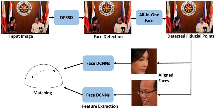
Figure 2: Our face recognition pipeline. We detect faces using our proposed DPSSD face detector (section 3.1). These detections are passed to the All-in-One Face network (section 3.2) which outputs facial keypoints for each face. These are used to align faces to canonical views. We pass these aligned faces through our face representation networks (section 3.3) and obtain the similarity between two faces using cosine similarity.

In this section, we discuss a state-of-the-art pipeline for face identification and verification, built by authors over the last eighteen months. An overview of the pipeline is given in figure 2. We first introduce the proposed DPSSD face detector in subsection 3.1. We then briefly summarize our face alignment method using the MTL approach. Lastly, we describe our approach for extracting identity features and using them for face identification and verification.

3.1 Deep Pyramid Single Shot Face Detector

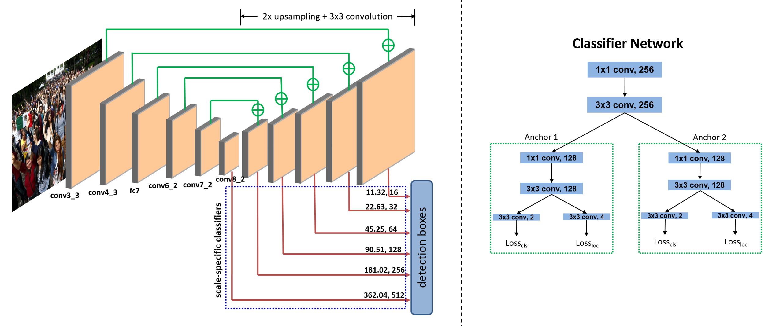
Figure 3: The network architecture for the proposed Deep Pyramid Single Shot Face Detector (DPSSD). Starting from the base SSD [6] network, we add upsampling layers in an hourglass manner [85] to generate rich contextual features for face detection. The faces are pooled from six different layers of the network, with 2 scales at each layer. The numbers on the red arrows denote the anchor sizes for a given layer. The classifier network generates the face detection probability scores as well as the normalized bounding box offsets for every anchor (shown on right).

We propose a novel DCNN-based face detector, called Deep Pyramid Single Shot Face Detector (DPSSD), that is fast and capable of detecting faces at a large variety of scales. It is especially good at detecting tiny faces. Since face detection is a special case of generic object detection, many researchers have used an off-the-shelf object detector and fine-tuned it for the task of face detection [27]. However, in order to design an efficient face detector, it is crucial to address the following differences between the tasks of face and object detection. First, the faces can occur at a much lower scale/size in an image compared to a general object. Typically, object detectors are not designed to detect at such a low resolution which is required for the task of face detection. Second, variations in the aspect ratio of faces are much less compared to those in a typical object. As faces incur less structural deformations compared to objects, they do not need any additional processing incorporated in object detection algorithms to handle multiple aspect ratios. We design our face detector to addresses these points.

We start with the Single Shot Detector (SSD) [6] trained on the truncated VGG-16 [58] network for the task of object detection. SSD [6] has a speed advantage over other object detectors like Faster R-CNN [5] since it is single stage and does not use proposals. The SSD approach is fully convolutional and generates a fixed number of bounding boxes and scores for the presence of faces. Additional convolutional layers are added to the end of the truncated VGG-16 [58] to detect objects at multiple scales. The objects are detected from multiple feature layers using different convolutional models for each layer. We modify the SSD [6] architecture and the approach in such a way that it is able to detect tiny faces efficiently. Fig. 3 shows the overall architecture of the proposed DPSSD face detector.

Anchor pyramid with fixed aspect-ratio: In order to detect faces at multiple scales, we leverage the feature pyramid structure inbuilt in the DCNN. We resize the input image such that the side with minimum length has a dimension of $512$. After every convolutional block, max pooling is performed which reduces the dimension of feature maps by half and doubles the stride. For instance, the feature maps at conv$3\_3$ layer have a minimum spatial dimension of $128$. Additionally, a unit stride in this layer corresponds to $4$ pixels stride in the original image. As shown in table III, initial layers of a DCNN have low stride in feature maps, which is beneficial for detecting tiny faces since small size anchors can be matched with high Jaccard overlap of $0.5$. However, features from these layers have less discriminative ability. On the other hand, features from deeper layers are semantically stronger, but do not provide good spatial localization because of the large stride value. Hence, we choose the anchor sizes and the corresponding feature maps for generating detections with an optimal combination of low spatial stride and highly discriminative features.

Layer	Stride (pixels)	Anchor-Sizes (pixels)	#boxes
conv$3\_3$	4	16/$\sqrt{2}$, 16	32768
conv$4\_3$	8	32/$\sqrt{2}$, 32	8192
fc$7$	16	64/$\sqrt{2}$, 64	2048
conv$6\_2$	32	128/$\sqrt{2}$, 128	512
conv$7\_2$	64	256/$\sqrt{2}$, 256	128
conv$8\_2$	128	512/$\sqrt{2}$, 512	32

TABLE III: Statistics for different layers of DPSSD. The sizes of the two anchors and the stride are measured in pixels.

We choose $12$ anchor boxes, each at a different scale. The largest anchor box has a size of $512$. Each anchor box maintains a scale factor of $\sqrt{2}$ with its next lower level in the hierarchy. We apply these anchor boxes to generate detections from $6$ different feature maps (see Table III). Small-sized anchor boxes are applied to shallower feature maps while large-sized anchor boxes are applied to deeper feature maps. Unlike SSD [6], we make use of the conv$3\_3$ layer for generating the detections since it has a high spatial resolution of $128$. This helps us in detecting tiny faces of size as low as $8$ pixels.

We fix the aspect ratio of every anchor box to the mean aspect-ratio for face ($0.8$). We compute this value from the WIDER Face [22] training dataset. For a given anchor size $a$, the anchor box $m\times n$ is calculated as:

$$m=\frac{a}{\sqrt{0.8}},~{}~{}~{}~{}~{}n=a\times\sqrt{0.8},$$ (1)

where $m$ is the width and $n$ is the height of the anchor box. Detection scores and bounding box offsets are provided at each location of the feature map for a given anchor box. Feature maps with larger spatial resolution result in more detection boxes. The number of detection boxes generated by every anchor layer for an image of size $512\times 512$, is also provided in table III. The conv$3\_3$ layer outputs the largest number of boxes since it has a spatial resolution of $128\times 128$. All of these generated boxes are passed through the classifier at the time of training.

Contextual Features from upsampling layers: It has been established that contextual information is useful for detecting tiny faces [36]. Although features from the conv$3\_3$ layer have appropriate spatial resolution for tiny face detection, they are neither semantically strong nor they contain contextual information. In order to provide contextual information, we add a stack of bilinear upsampling and convolution layer at the end of the SSD [6] network. The $6$ chosen layers (Table III) are then added element-wise to these upsampled layers (see Fig. 3). Thus, the features become rich in both semantics and localization. The final detection boxes are generated from these upsampled layers using the anchor box matching technique.

Every output level generates two sets of detections, one for each anchor box corresponding to the given layer. A classifier network (see Fig. 3 right) is attached to all the $6$ output feature maps, that provides the classification probabilities and bounding box offsets corresponding to each of the $12$ anchor boxes. The classifier network is branched into two to handle each anchor box separately. These branches are further subdivided into classification and regression subnetworks.

3.1.1 Training

We use the training set of WIDER Face [22] dataset to train our face detector. The network is initialized with the SSD [6] model for object detection. The new layers that are added are initialized randomly. We use a batch size of $8$. The initial learning rate is set to $0.001$ which is decreased by $0.5$ after $30k$, $50k$ and $60k$ iterations. Training is carried out till $70k$ iterations. The matching strategy is similar to SSD [6]. A location in the predictor feature map is labeled as positive class ($y_{c}=1$) if the anchor box for that location has an Intersection-over-Union (IoU) overlap of $0.5$ or more with any ground truth face. All the other locations are labeled as negative class ($y_{c}=0$). For all the positive classes, we also perform bounding box regression. We use the binary cross-entropy loss for face classification and smooth-L1 loss for bounding box regression. The overall loss ($L$) is a weighted sum of classification loss ($L_{cls}$) and regression loss ($L_{loc}$) as shown in (2), (3) and (4). We use Caffe [86] library to train our network.

$$L_{cls}=-y_{c}\cdot\log(p_{c})-(1-y_{c})\cdot\log(1-p_{c}),$$ (2)

$$L_{loc}=\sum\limits_{i\in\{x,y,w,h\}}~{}\mathrm{smooth}_{L1}~{}(t_{i}-v_{i}),$$ (3)

$$L=L_{cls}+\lambda\cdot y_{c}\cdot L_{loc},$$ (4)

where $y_{c}$ is the class label, $p_{c}$ is the softmax probability obtained from the network, $v=\{v_{x},v_{y},v_{w},v_{h}\}$ denote the ground-truth normalized bounding box regression targets while $t=\{t_{x},t_{y},t_{w},t_{h}\}$ are the bounding box offsets predicted by the network. The value of $\lambda$ is chosen to be $1$. The $\mathrm{smooth}_{L1}$ loss is defined in (5).

$$\mathrm{smooth}_{L1}(x)=\begin{cases}0.5x^{2}&\quad\text{if }|x|<1\\ |x|-0.5&\quad\text{otherwise}\\ \end{cases}$$ (5)

The total number of detection boxes generated from an image is $43,680$. Out of these, only a few boxes (around $10$-$50$) correspond to the positive class while others form the negative class. To avoid this large class imbalance we select only a few negative boxes such that the ratio of positive to negative class is $1:3$. We use hard negative mining to select these negative boxes as proposed in [6]. We use the data augmentation technique proposed in [6] to make the detector more robust to various face sizes.

3.1.2 Testing

At test time, the input image is resized such that the minimum side has the dimension of $512$ pixels. The aspect ratio of the image is not changed. The image is then passed through the trained DPSSD face detector to get the detection scores and bounding box co-ordinates for different locations in the image. Non-maximum suppression (NMS) with threshold of $0.6$ is used to filter out the redundant boxes. Since the outputs are generated in a single pass of the network, the total processing time is very low ($100ms$). To further improve the detection performance, we construct the image pyramid as discussed in HR [36] face detector. A sample face detection output using the proposed DPSSD is shown in Fig. 4. Performance evaluations of different face detection datasets are discuss in Section 4.

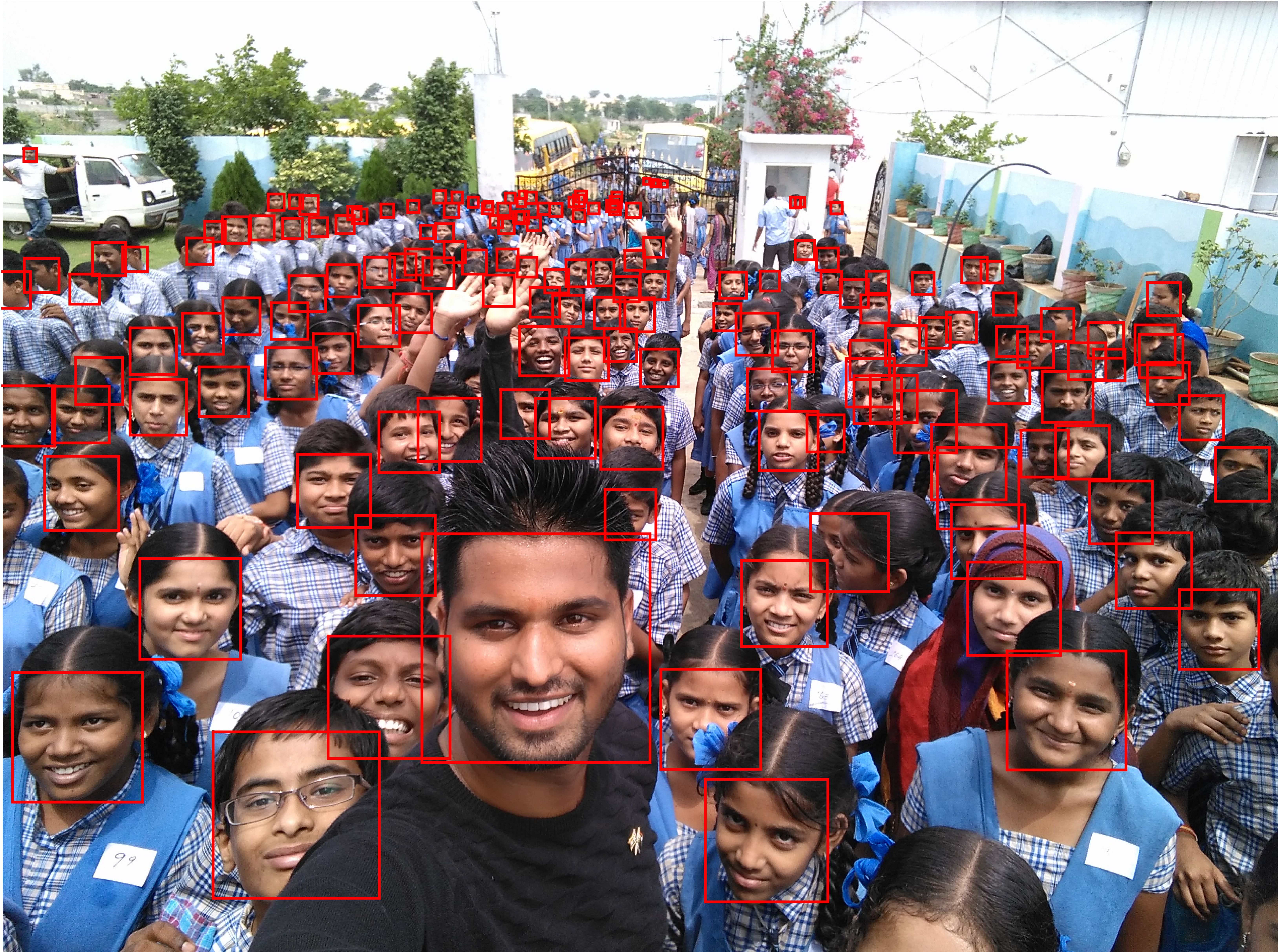
Figure 4: A sample output for our proposed DPSSD.

For the proposed face recognition pipeline, we use the results of both DPSSD and SSD for faces, as our detectors to capture faces across as many scales as possible.

3.2 Face Alignment using All-In-One Face

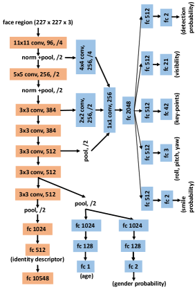
Figure 5: The All-In-One Face network architecture.

The proposed system for face identification and verification uses the All-in-One Face framework [8] for keypoint localization. The All-In-One Face [8] is a recent method that simultaneously performs the tasks of face detection, landmarks localization, head-pose estimations, smile and gender classification, age estimation and face recognition and verification. The model is trained jointly for all these tasks in a MTL framework, which builds up a synergy that helps in improving the performance of the individual tasks.

Due to the lack of a single dataset which contains annotations for each task, various sub-networks were trained with different datasets. These sub-networks share parameters among them. This ensures that the shared parameters adapt to all the tasks instead of being task-specific. These sub-networks are fused into a single All-in-One Face CNN at test time. Table IV gives some details of the datasets used for training All-in-One Face CNN. The complete network is trained end-to-end using task-specific loss functions. Figure 6 shows some representative outputs of the All-in-One Face CNN.

Dataset	Facial Analysis Task	# training samples
CASIA [14]	Identification, Gender	490,356
MORPH [87]	Age, Gender	55,608
IMDB+WIKI [88]	Age, Gender	224,840
Adience [89]	Age	19,370
CelebA [72]	Smile, Gender	182,637
AFLW [90]	Detection, Pose, Fiducials	20,342
Total		993,153

TABLE IV: Datasets used for training All-In-One Face.

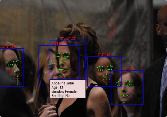
Figure 6: Sample outputs from the All-In-One Face [8] CNN for IJB-A  [66].

The All-In-One network architecture uses the pre-trained face identification network from Sankaranarayanan et al. [25], which contains seven convolutional layers followed by three fully connected layers. This network is used as a backbone to train the face identification task. The parameters from the first six convolutional layers of this network are shared among the other face-related tasks as shown in figure 5. A CNN pre-trained on face identification task provides better initialization for a generic face analysis task, since the filters retain discriminative face information.

The face-related tasks used for training are divided into two categories: 1) subject-independent tasks of face detection, landmarks localization, pose estimation, and smile prediction; 2) subject-dependent tasks of gender classification, age estimation and face recognition. The subject-dependent tasks require fine-grained features for classification, and hence need semantically stronger features present in the deeper layers of the network. On the other hand, subject-independent tasks are more localization oriented which need the features from shallower layers of the network. Keeping these requirements in mind, the subject-independent features are pooled from the first, third and fifth convolutional layers, while subject-dependent features are pooled from deeper layers (see Fig. 5).

Although All-In-One Face [8] provides outputs for seven different face-related tasks, we use only the facial keypoints generated by this network in our face recognition pipeline. Once we obtain the keypoints for every face in an image or a video frame, we align the faces to normalized the canonical coordinates to mitigate the effects of in-plane rotation and scaling. These aligned faces are then passed to the face recognition module for further processing.

3.3 Face Identification and Verification

In this subsection, we discuss our approach for face identification and verification. We use Crystal Loss [24] to train deep networks for the task of face classification. Identity features are then extracted for a face image from the penultimate layer of the trained networks. These features undergo triplet embedding [25] and fusion to generate a template representation for an identity.

3.3.1 Crystal Loss for Training CNNs

Until recently, almost all face identification/verification networks were trained in the classification setting using a softmax loss function. However, softmax loss is not ideal for training networks for face representation. Softmax loss does not optimize the features to be similar for faces of the same person and dissimilar for faces of different people. This leads to reduced performance. To alleviate these issues Ranjan et al. introduced the crystal loss function [24] for training networks used for unconstrained face verification and identification. The main idea behind this is to constrain the features to lie on a hypersphere of a fixed radius. This ensures that the features learnt are well-separated for different identities but close for same identities. Scaling the features means that every image has a feature with the same scale. Contrast this with the softmax loss where high quality images usually give a feature with higher norm. This causes softmax loss to give more attention to good quality images. This issue is also alleviated by the crystal loss which gives equal importance to high and low quality images.

The objective function for a network trained with crystal loss can be written as:

minimize $$-\frac{1}{M}\sum_{i=1}^{M}\log\frac{e^{W^{T}_{y_{i}}f(\mathbf{X}_{i})+b_{y_{i}}}}{\sum_{j=1}^{C}e^{W^{T}_{j}f(\mathbf{X}_{i})+b_{j}}}$$ (6)

subject to $$\lVert f(\mathbf{X}_{i})\rVert_{2}=\alpha,\forall i=1,2,\dots M,$$

where $\mathbf{X}_{i}$ is the input image with label $y_{i}$, $M$ is the batch size, $f(\mathbf{X}_{i})$ is the feature representation from the network, $C$ is the number of classes, $W$ and $b$ are the weights of the classification layer of the network, and $\alpha$ is the scale of the feature representation.

This objective can be easily integrated into the network by simply normalizing the feature and scaling it by $\alpha$ and applying softmax loss over this scaled representation. This module is fully differentiable and can be inserted into any network trained using softmax loss.

3.3.2 Training Datasets

We use the Universe face dataset from [13] for training our face representation networks. This is a combination of UMDFaces images [16], UMDFaces video frames [15], and curated MS-Celeb-1M [91]. The Universe dataset contains about 5.6 million images of about 58,000 identities. This includes about 3.5 million images from MS-Celeb-1M, 1.8 million video frames from UMDFaces videos, and 300,000 images from UMDFaces. This dataset has the advantage of being a combination of different datasets which makes networks trained using this dataset generalize better. Another advantage is that it contains both still images and video frames. This makes the networks more robust for test datasets which contain both.

3.3.3 Face Representation

We use two networks for feature representation. We do a score-level fusion of the scores obtained from these networks. Using an ensemble of networks leads to more robust representations and better performance. We next describe the two networks along with their respective training details. These two networks are based on a ResNet-101 [3], and Inception ResNet-v2 [92].

For pre-processing the detected faces, we crop and resize the aligned faces to each network’s input dimensions. For data augmentation, we apply random horizontal flips to the input images.

ResNet-101 (RG1)
We train a ResNet-101 deep convolutional neural network with PReLU activations after every convolution layer. Since we use the Universe dataset for training the network, we use a $58,000$-way classification layer with crystal loss. For this network, we set the $\alpha$ parameter to $50$ and the batch size was $128$. The learning rate started at $0.1$ and was reduced by a factor of 0.2 after every $50k$ iterations. The network was trained for a total of $250k$ iterations. We use a $512$-D layer as the feature layer and use TPE [25] to find a 128-D embedding with was trained with the UMDFaces dataset.

Inception ResNet-v2 (A)
The Inception ResNet-v2 network was also trained with the Universe dataset. This network has 244 convolution layers. We add a $512$-D feature layer after these and then a final classification layer. We again use crystal loss with $\alpha=40$. The initial learning rate was $0.1$ and reduced by a factor of $0.2$ after every $50k$ iterations. We trained the network for $120k$ iterations with a batch-size of $120$ on 8 NVIDIA Quadro P6000 GPUs. We resize the inputs to $299\times 299$. Similar to the ResNet, we use UMDFaces to train a final 128-D embedding with TPE.

3.3.4 Feature Fusion

Template Feature
For both face verification and identification, we need to compare template features. To obtain feature vectors for a template, we first average all the features for a media in the template. We further average these media-averaged features to get the final template feature.

Score-level Fusion
To get the similarity between two templates, we average the similarities obtained by our two networks.

4 Experimental Results

In this section, we first report face detection results for the proposed detector on four datasets. We also report experimental results for face identification and verification on four challenging evaluation datasets, viz., IJB-A [66], IJB-B [73], IJB-C [74], and the IARPA Janus Challenge Set 5 (CS5). We show that the proposed system achieves state-of-the-art or near results on most of the protocols. In the following sections we describe the evaluation datasets and protocols. We also describe the changes to the system we made if there are any.

4.1 Face Detection

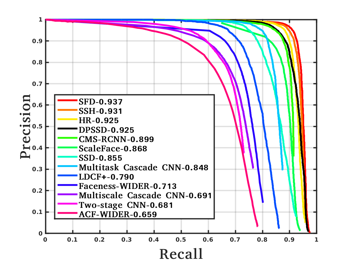
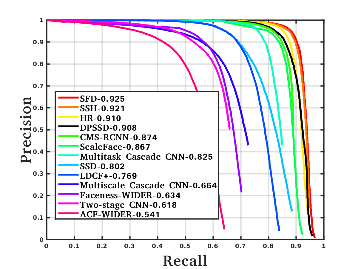
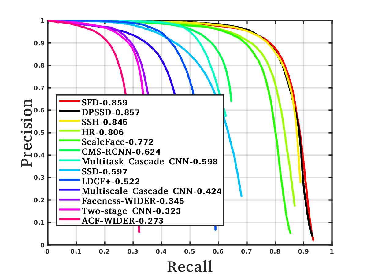
(a) Easy                                        (b) Medium                                        (c) Hard

Figure 7: Performance evaluation on the WIDER Face [22] validation dataset for (a) Easy, (b) Medium, and (c) Hard faces. The numbers in the legend represent the mean average precision (mAP) for the corresponding method.

We evaluated the proposed DPSSD face detector on four challenging face detection datasets: WIDER Face [22], Unconstrained Face Detection Dataset (UFDD) [93], Face Detection Dataset and Benchmark (FDDB) [94] and Pascal Faces [95]. We achieve state-of-the-art performance on Pascal Faces [95] dataset, and competing results on WIDER [22], UFDD [93] and FDDB [94] datasets.

4.1.1 WIDER Face Dataset Results

The dataset contains $32,203$ images with $393,703$ face annotations, out of which $40\%$ images are used for training, $10\%$ for validation, and remaining $50\%$ for test. It contains rich annotations, including occlusions, poses, event categories, and face bounding boxes. The faces posses large variations in scale, pose and occlusion. The dataset is extremely challenging for the task of tiny face detection, since the face width can be as low as $4$ pixels. We use the training set to train the face detector and evaluate its performance on the validation set. Fig. 7 provides the comparison of recently published face detection algorithms with the proposed DPSSD.

We compare the performance of DPSSD with S³FD [33], SSH [7], HR [36], CMS-RCNN [96], ScaleFace [32], Multitask Cascade [82], LDCF+ [97], Faceness [98], Multiscale Cascade [22], Two-stage CNN [22], and ACF [99]. We observe that DPSSD achieves competing performance with state-of-the-art methods (S³FD [33], SSH [7], and HR [36]). It achieves a mean average precision (mAP) of $0.925$ and $0.908$ on easy and medium difficulty set, respectively. On the hard set, it performs very close to the best performing method (S³FD [33]) with the mAP of $0.857$.

We also compare our method with the baseline face detector trained by fine-tuning SSD [100]. We outperform SSD [100] on easy, medium as well as hard set. Particularly on the hard set, DPSSD improves the mAP by a factor of $44\%$ over the SDD [100]. It shows that redesigning anchor pyramid with fixed aspect ratio, and adding the upsampling layers helps tremendously in boosting the performance of face detection.

4.1.2 UFDD Dataset Results

UFDD is a recent face detection dataset that captures several realistic issues not present in any existing dataset. It contains face images with weather-based degradations (rain, snow and haze), motion blur, focus blur, etc. Additionally, it contains distractor images that either contain non-human faces such as animal faces or no faces at all, which makes this dataset extremely challenging. It contains a total of $6,425$ images with $10,897$ face annotations. We compare our proposed method with S³FD [33], SSH [7], HR [36], and Faster-RCNN [27] (see Fig. 8). Similar to WIDER Face [22] dataset, we achieve competing results with mAP of $0.706$. Note that our algorithm is not fine-tuned on the UFDD dataset.

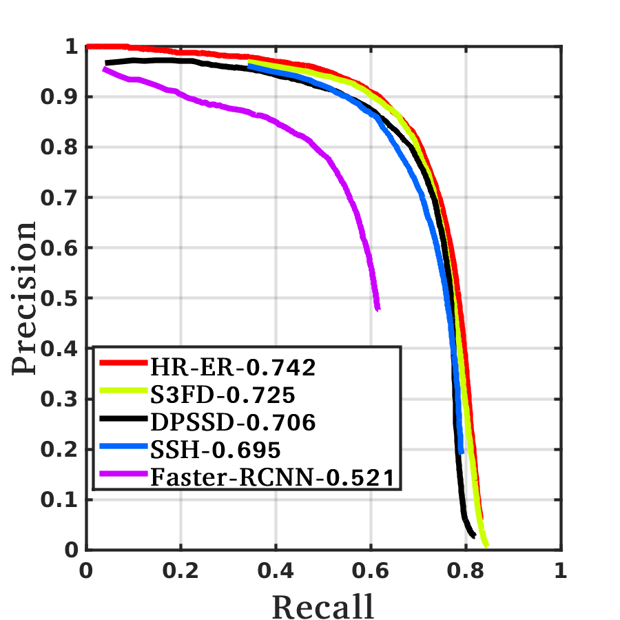
Figure 8: Performance evaluation on the UFDD [93] dataset. The numbers in the legend represent the mAP for the corresponding method.

4.1.3 FDDB Dataset Results

The FDDB dataset [94] is a benchmark for unconstrained face detection. It consists of $2,845$ images containing a total of $5,171$ faces collected from news articles on the Yahoo website. The images were manually localized for generating the ground truth. The dataset has two evaluation protocols - discrete and continuous which essentially correspond to coarse match and precise match between the detection and the ground truth, respectively. We evaluate the performance of our method on the discrete protocol using the Receiver Operating Characteristic (ROC) curves, as shown in Fig. 9.

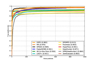
Figure 9: Performance evaluation on the FDDB [94] dataset. The numbers in the legend represent the mAP for the corresponding method.

We compare the performance of different face detectors such as S³FD [33], HR [36], Faster-RCNN [27], All-In-One Face [8], LDCF+ [97], DP2MFD [9], Faceness [98], HyperFace [10], Headhunter [101], DPM [101], and Joint Cascade [79]. As can be seen from the figure, our method exhibits competing performance with state-of-the-art methods (S³FD [33] and HR [36]) and achieves a mAP of $0.969$. It should be noted that our method does not use any fine-tuning or bounding box regression specific to the FDDB dataset.

4.1.4 PASCAL Faces Dataset Results

The PASCAL faces [95] dataset was collected from the test set of the person layout dataset which is a subset of PASCAL VOC [102]. The dataset contains $1,335$ faces from $851$ images with large variations in appearance and pose. Fig. 10 compares the performance of different face detectors on this dataset. From the figure, we observe that our proposed DPSSD face detector achieves the best mAP of $96.11\%$ on this dataset.

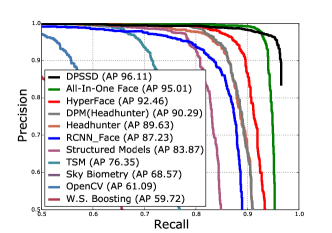
Figure 10: Performance evaluation on the Pascal Faces [95] dataset. The numbers in the legend represent the mAP for the corresponding method.

Table V lists the locations of the results for different datasets and verification and identification evaluation tasks.

Task	IJB-A	IJB-B	IJB-C	CS5
1:1 Verification	Table VII	Table IX	Table XII	Table XVI
1:N Search	Table VIII	Table X	Table XIII	Table XVII
Wild Probe Search	-	-	Table XIV	Table XVIII

TABLE V: Locations of all results for face verification and identification.

In the following sections, ROC curves are used to measure the performance of verification (1:1 matching) methods and CMC scores are used for evaluating identification (1:N search). The IJB-A, IJB-B, IJB-C, and CS5 datasets contain a gallery and a probe which leads to evaluation using all positive and negative pairs. This is different from LFW [59] and YTF [103] where only a few negative pairs are used to evaluate verification performance. Another difference between LFW/YTF and the evaluation datasets here is the inclusion of templates instead of only single images. A template is a collection of images and video frames of a subject. These datasets are much more challenging than older datasets due to extreme variations in pose, illumination, and expression.

4.2 IJB-A

The IJB-A dataset contains 500 subjects with 5,397 images and 2,042 videos split into 20,412 frames. This dataset is a very difficult dataset owing to the presence of extreme pose, viewpoint, resolution, and illumination variations. Additionally, mixing still images and video frames causes difficulties for models trained with only one of these modalities due to domain shift. An identity in this dataset is represented as a template. A template is a set of face images instead of just a single image. This set can contain still images and video frames. Also note that each subject can have multiple templates in the dataset. The evaluation for this dataset contains for 1:1 verification and 1:N mixed search protocols. Table VI gives brief descriptions of the two tasks. The dataset is divided into 10 splits, each with $333$ randomly selected subjects for training and $167$ subjects for testing. To represent each template, we generate a common representation by fusing features of all the faces in the template. We compute the similarity scores using all the networks and then do a score-level fusion as described in 3.3.4. Table VII gives the results from our system for the verification task for IJB-A and table VIII gives the results for 1:N mixed search. We achieve state-of-the-art results for every setting.

Task	Desciption
1:1 Verification	Verify if the given pair of templates belong to the same subject. Templates are comprised of mixed media (frames and stills)
1:N Mixed Search	Open set identification protocol using mixed media (frames and stills) as probe and two galleries G1, and G2.

TABLE VI: IJB-A and IJB-B task descriptions

	True Accept Rate (%) @ False Accept Rate
Method	0.0001	0.001	0.01	0.1
Casia [104]	-	51.4	73.2	89.5
Pose [61]	-	-	78.7	91.1
NAN [67]	-	88.1	94.1	97.8
3d [105]	-	72.5	88.6	-
DCNNfusion [12]	-	76.0	88.9	96.8
DCNNtpe [25]	-	81.3	90.0	96.4
DCNNall [8]	-	78.7	89.3	96.8
All + TPE [8]	-	82.3	92.2	97.6
TP [106]	-	-	93.9	-
RX101l2+tpe [65]	90.9	94.3	97.0	98.4
OursA	91.7	95.3	96.8	98.3
OursRG1	91.4	94.8	97.1	98.5
Fusion (Ours)	92.1	95.2	96.9	98.4

TABLE VII: IJB-A Verification. A is our Inception ResNet-v2 model and RG1 is our ResNet-101 model.

	TPIR (%) @ FPIR		Retrieval Rate (%)
Method	0.01	0.1	Rank=1	Rank=5	Rank=10
Casia [104]	38.3	61.3	82.0	92.9	-
Pose [61]	52.0	75.0	84.6	92.7	94.7
BL [107]	-	-	89.5	96.3	-
NAN [67]	81.7	91.7	95.8	98	98.6
3d [105]	-	-	90.6	96.2	97.7
DCNNfusion [12]	65.4	83.6	94.2	98.0	98.8
DCNNtpe [25]	75.3	83.6	93.2	-	97.7
DCNNall [8]	70.4	83.6	94.1	-	98.8
ALL + TPE [8]	79.2	88.7	94.7	-	98.8
TP [106]	77.4	88.2	92.8	-	98.6
RX101l2+tpe [65]	91.5	95.6	97.3	-	98.8
OursA	91.4	96.1	97.3	98.2	98.5
OursRG1	91.6	96.0	97.4	98.5	98.9
Fusion (Ours)	92.0	96.2	97.5	98.6	98.9

TABLE VIII: IJB-A 1:N Mixed Search. A is our Inception ResNet-v2 model and RG1 is our ResNet-101 model.

4.3 IJB-B

The IJB-B dataset [73], which extends IJB-A, contains about $22,000$ still images and $55,000$ video frames spread over $1,845$ subjects. Evaluation is done for the same tasks as IJB-A, viz., 1:1 verification, and 1:N identification (table VI). The IJB-B verification protocol consists of $8,010,270$ pairs between templates in the galleries (G1 and G2) and the probe templates. Out of these 8 million are impostor pairs and the rest $10,270$ are genuine comparisons. Table IX gives verifications results and table X gives identification results.

	True Accept Rate (%) @ False Accept Rate
Method	$10^{-7}$	$10^{-6}$	$10^{-5}$	$10^{-4}$	$10^{-3}$	$10^{-2}$	$10^{-1}$
GOTS [73]	-	-	-	16.0	33.0	60.0	-
VGGFaces [63]	-	-	-	55.0	72.0	86.0	-
FPN [108]	-	-	-	83.2	91.6	96.5	-
Light CNN-29 [109]	-	-	-	87.7	92.0	95.3	-
VGGFace2 [21]	-	-	70.5	83.1	90.8	95.6	-
Center Loss Features [63]	8.8	31.0	63.6	80.7	90.0	95.1	98.4
OursA	2.9	27.7	61.6	89.1	94.3	97.0	98.7
OursRG1	6.2	48.4	80.4	89.8	94.4	97.2	98.9
Fusion (Ours)	4.4	45.6	77.8	90.3	94.6	97.3	98.9

TABLE IX: IJB-B Verification. A, RG1, and Fusion are our Inception ResNet-v2, ResNet-101, and Fused features respectively.

	TPIR (%) @ FPIR (For G1, G2)		Retrieval Rate (%) (For G1, G2)
Method	0.01	0.1	Rank=1	Rank=5	Rank=10
GOTS [73]	-	-	42.0	-	62.0
VGGFace [63]	-	-	78.0	-	89.0
FPN [108]	-	-	91.1	-	96.5
Light CNN-29 [109]	-	-	91.9	94.8	-
VGGFace2 [21]	74.3	86.3	90.2	94.6	95.9
Center Loss Features [63]	75.5, 67.7	87.5, 82.8	92.2, 86.0	95.4, 92.5	96.2, 94.4
OursA	83.1, 75.5	93.6, 89.3	95.5, 90.8	97.5, 94.2	98.0, 95.8
OursRG1	86.9, 78.6	94.0, 89.1	95.6, 91.5	97.7, 95.4	98.0, 96.5
Fusion (Ours)	88.2, 79.4	94.3, 89.7	95.8, 91.8	97.7, 95.2	98.1, 96.4

TABLE X: IJB-B 1:N Mixed Search. A and RG1 are our Inception ResNet-v2 and ResNet-101 models respectively. Note that the retrieval rates for some past methods are average over G1 and G2.

4.4 IJB-C

The IJB-C evaluation dataset [74] further extends IJB-B. It contains $31,334$ still images and $117,542$ video frames of $3,531$ subjects. In addition to the evaluations from IJB-B, this dataset evaluates end-to-end recognition. Table XI gives the descriptions of the evaluated tasks for IJB-C. There are about $20,000$ genuine comparisons, and about $15.6$ million impostor pairs in the verification protocol. For the 1:N mixed search protocol, there are about $20,000$ probe templates. In table XII we list the results of our system for 1:1 verification. Similarly, in table XIII we give results for 1:N mixed search. We also report the 1:N wild probe search results in table XIV.

Task	Desciption
1:1 Verification	Verify if the given pair of templates belong to the same subject. Templates are comprised of mixed media (frames and stills)
1:N Mixed Search	Open set identification protocol using mixed media (frames and stills) as probe and two galleries G1, and G2.
Wild Probe Search	Identify subjects of interest from a collection of still images and frames. This task also uses the two galleries G1, and G2.

TABLE XI: IJB-C task descriptions

	True Accept Rate (%) @ False Accept Rate
Method	$10^{-8}$	$10^{-7}$	$10^{-6}$	$10^{-5}$	$10^{-4}$	$10^{-3}$	$10^{-2}$	$10^{-1}$
Center Loss Features [63]	36.0	37.6	66.1	78.1	85.3	91.2	95.3	98.2
OursA	16.5	19.5	43.6	77.6	91.9	95.6	97.8	99.0
OursRG1	60.6	67.4	76.4	86.2	91.9	95.7	97.9	99.2
Fusion (Ours)	54.1	55.9	69.5	86.9	92.5	95.9	97.9	99.2

TABLE XII: IJB-C Verification. A is our Inception ResNet-v2 model and RG1 is our ResNet-101 model. Fusion is the fusion of the two features.

	TPIR (%) @ FPIR (For G1, G2)		Retrieval Rate (%) (For G1, G2)
Method	0.01	0.1	Rank=1	Rank=5	Rank=10
Center Loss Features [63]	79.1, 75.3	86.4, 84.2	91.7, 89.8	94.6, 93.6	95.6, 94.9
OursA	87.7, 82.4	93.5, 91.0	95.7, 92.8	97.4, 95.4	97.9, 96.4
OursRG1	88.0, 84.2	93.2, 90.6	95.9, 93.2	97.6, 96.1	98.1, 97.0
Fusion (Ours)	89.6, 85.0	93.8, 91.3	96.2, 93.6	97.7, 96.2	98.2, 96.9

TABLE XIII: IJB-C 1:N Mixed Search. A and RG1 are our models described in section 3.3.3.

	Retrieval Rate (%) (For G1, G2)
Method	Rank=1	Rank=2	Rank=5	Rank=10	Rank=20	Rank=50
OursA	91.1, 86.9	93.0, 89.0	94.8, 91.1	95.8, 92.5	96.5, 93.8	97.4, 95.3
OursRG1	90.8, 86.3	93.0, 88.8	95.0, 91.1	96.0, 92.6	96.7, 93.9	97.5, 95.5
Fusion (Ours)	91.8, 87.5	93.6, 89.7	95.3, 91.6	96.3, 93.0	97.0, 94.4	97.7, 95.8

TABLE XIV: IJB-C Wild Probe Search. Our models and fusion method are described in sections 3.3.3 and 3.3.4.

4.5 CS5

We evaluated on the (as-yet-unreleased to public) JANUS Challenge Set 5 dataset also. We give the task descriptions for this dataset in table XV. This dataset consists of $2,875,950$ still images. This dataset also provides a training set consisting of $235,616$ identity clusters and $981,753$ images. Note that we did not use this training set for training our networks. The still image verification protocol contains $547,131$ templates with $332,574$ genuine matches, and $822,354,805$ imposter matches. For the 1:N identification task, there are $332,574$ probe templates. Gallery, G1 has $1,106,778$ identity clusters and G2 has $1,107,779$ identity clusters. Tables XVI, XVII, and XVIII give results for 1:1 verification, 1:N identification, and 1:N end-to-end identification respectively.

Note that we are unable to compare the performance of the proposed approach against other methods for IJB-C and CS5 due to restrictions on publishing competitor’s results.

Task	Desciption
1:1 Still Image Verification	Templates are comprised of only still images.
1:N Still Image Identification	Open set identification protocol using still images as probe and two galleries G1, and G2 augmented with 1M distractors.
1:N end-to-end Still Image	Identify identity clusters of interest from a collection of still images. This task also uses the two galleries G1, and G2.

TABLE XV: IARPA Janus Challenge Set 5 (CS5) task descriptions

	True Accept Rate (%) @ False Accept Rate
Method	$10^{-8}$	$10^{-7}$	$10^{-6}$	$10^{-5}$	$10^{-4}$	$10^{-3}$	$10^{-2}$	$10^{-1}$
OursA	52.44	78.99	94.88	97.34	98.18	98.74	99.28	99.75
OursRG1	71.52	89.68	95.20	97.28	98.19	98.79	99.36	99.78
Fusion (Ours)	70.72	90.74	95.80	97.49	98.25	98.80	99.35	99.78

TABLE XVI: CS5 1:1 Verification. A and RG1 are our Inception ResNet-v2 and ResNet-101 models respectively. Both of these models are trained with Crystal Loss.

	TPIR (%) @ FPIR				Retrieval Rate (%)
	(Average for G1 and G2)				(Average for G1 and G2)
Method	0.0001	0.001	0.01	0.1	Rank=1	Rank=5	Rank=10	Rank=20
Fusion (Ours)	29.96	75.90	86.76	95.59	96.99	97.76	97.92	98.06

TABLE XVII: CS5 1:N Identification

	Retrieval Rate (%) (Average for G1 and G2)
Method	Rank=1	Rank=2	Rank=5	Rank=10	Rank=20	Rank=50
Fusion (Ours)	97.18	97.65	97.90	98.04	98.16	98.31

TABLE XVIII: CS5 1:N end-to-end still image identification

5 Conclusions

In this paper, we presented an overview of modern face recognition systems based on deep CNNs. We discussed all parts of a face recognition pipeline and the state-of-the-art in those. We also presented details of our face recognition system which uses an ensemble of two networks for feature representation. Face detection and keypoint localization for in our pipeline is done using the All-in-One CNN. We discussed training and datasets details for our system and how it connects to existing work on face recognition. We presented results of our system for four challenging datasets, viz., IJB-A, IJB-B, IJB-C, and IARPA Janus Challenge Set 5 (CS5). We show that our ensemble based system achieves near state-of-the-art results.

However, several issues remain unresolved even now. There is a need to develop theoretical understanding of face recognition systems based on DCNNs. Given the multitude of loss functions used to train these networks, we need to develop a unified framework which can put all of them in context to each other. Domain adaptation and dataset bias is also an issue for current face recognition systems. These systems are usually trained on a dataset and work well for similar test sets. However, networks trained on one domain don’t perform well for others. We trained our system on a combination of different datasets. This made the trained models more robust. Training CNNs currently takes several hours to days. There is a need to develop more efficient architectures and implementations of CNNs which can be trained faster.

Rajeev Ranjan received the B.Tech. degree in Electronics and Electrical Communication Engineering from Indian Institute of Technology Kharagpur, India, in 2012. He is currently a Research Assistant at University of Maryland College Park. His research interests include face detection, face recognition and machine learning. He received Best Poster Award at IEEE BTAS 2015. He is a two-time recipient of UMD Outstanding Invention of the Year award in the area of Information Science. He received the 2016 Jimmy Lin Award for Invention.

Ankan Bansal (B.Tech-M.Tech, IIT Kanpur, 2015) is a PhD student at the University of Maryland, College Park. His research interests include multi-modal learning, action understanding, and face analysis. He was awarded the Clark School of Engineering Distinguished Graduate Fellowship, 2015-2016.

Jingxiao Zheng (B.Eng, SEU, Nanjing, 2012, M.S., UMD, 2014) is currently a research assistant in the Institute for Advanced Computer Studies at the University of Maryland, College Park. His advisor is Prof. Rama Chellappa. His research interests include deep learning, face recognition, and action recognition.

Hongyu Xu (B.Eng, USTC, 2012, M.S., UMD, 2016) is currently a research assistant in the Institute for Advanced Computer Studies at the University of Maryland, College Park, advised by Prof. Rama Chellappa. He is a former research intern with Snap Research (summer, fall 2017) and Palo Alto Research Center (PARC) (summer 2014). His research interests include object detection, deep learning, dictionary learning, face recognition, object classification, and domain adaptation.

Joshua Gleason (B.S. Elec. Eng., B.S. Comp. Sci., UNR, 2013) is a PhD student at the University of Maryland, College Park and is advised by Prof. Rama Chellappa. His current research interests include face recognition, transfer learning, and general machine learning and computer vision topics.

Boyu Lu (B.Eng, USTC, 2012) is currently a research assistant at the University of Maryland, College Park. His research interests include face recognition, deep learning, and domain adaptation.

Anirudh Nanduri (B.Tech, IIT Bombay, 2015) is a PhD student at the University of Maryland, College Park. His research interests include geometric deep learning, medical image processing, face analysis and action recognition. He was awarded the Clark School of Engineering Distinguished Graduate Fellowship, 2015-2016.

Jun-Chen Chen (Ph.D., UMD, 2016) is a postdoctoral research fellow at the University of Maryland Institute for Advanced Computer Studies (UMIACS). His current research interests include computer vision and machine learning with applications to face recognition and facial analysis. He was a recipient of ACM Multimedia best technical full paper award, 2006.

Carlos D. Castillo (Ph.D., UMD, 2012) is an assistant research scientist at the University of Maryland Institute for Advanced Computer Studies (UMIACS). His current research interests include stereo matching, multi-view geometry, face detection, alignment and recognition.

Rama Chellappa (Ph.D., Purdue University, 1981) is a Distinguished University Professor, and a Minta Martin Professor of Engineering of Electrical and Computer Engineering Department at University of Maryland, College Park. His current research interests are face and gait analysis, 3-D modeling from video, image and video-based recognition and exploitation, compressive sensing, and hyper spectral processing. He received the Society, Technical Achievement and Meritorious Service Awards from the IEEE Signal Processing Society.

References

- [1] A. Krizhevsky, I. Sutskever, and G. E. Hinton, “Imagenet classification with deep convolutional neural networks,” in Advances in Neural Information Processing Systems, 2012, pp. 1097–1105.
- [2] C. Szegedy, W. Liu, Y. Jia, P. Sermanet, S. Reed, D. Anguelov, D. Erhan, V. Vanhoucke, and A. Rabinovich, “Going deeper with convolutions,” arXiv preprint arXiv:1409.4842, 2014.
- [3] K. He, X. Zhang, S. Ren, and J. Sun, “Deep residual learning for image recognition,” in IEEE Conference on Computer Vision and Pattern Recognition (CVPR), 2016, pp. 770–778.
- [4] R. Girshick, J. Donahue, T. Darrell, and J. Malik, “Rich feature hierarchies for accurate object detection and semantic segmentation,” in IEEE Conference on Computer Vision and Pattern Recognition, 2014, pp. 580–587.
- [5] S. Ren, K. He, R. Girshick, and J. Sun, “Faster r-cnn: Towards real-time object detection with region proposal networks,” in Advances in neural information processing systems, 2015, pp. 91–99.
- [6] W. Liu, D. Anguelov, D. Erhan, C. Szegedy, S. Reed, C.-Y. Fu, and A. C. Berg, “Ssd: Single shot multibox detector,” in European Conference on Computer Vision (ECCV), 2016, pp. 21–37.
- [7] M. Najibi, P. Samangouei, R. Chellappa, and L. Davis, “Ssh: Single stage headless face detector,” in Proceedings of the IEEE Conference on Computer Vision and Pattern Recognition, 2017, pp. 4875–4884.
- [8] R. Ranjan, S. Sankaranarayanan, C. D. Castillo, and R. Chellappa, “An all-in-one convolutional neural network for face analysis,” IEEE International Conference on Automatic Face and Gesture Recognition (FG), 2017.
- [9] R. Ranjan, V. M. Patel, and R. Chellappa, “A deep pyramid deformable part model for face detection,” in Biometrics Theory, Applications and Systems (BTAS), 2015 IEEE 7th International Conference on. IEEE, 2015, pp. 1–8.
- [10] R. Ranjan, V. Patel, and R. Chellappa, “Hyperface: A deep multi-task learning framework for face detection, landmark localization, pose estimation, and gender recognition,” IEEE Transactions on Pattern Analysis and Machine Intelligence, 2017.
- [11] A. Kumar, R. Ranjan, V. Patel, and R. Chellappa, “Face alignment by local deep descriptor regression,” arXiv preprint arXiv:1601.07950, 2016.
- [12] J. Chen, R. Ranjan, S. Sankaranarayanan, A. Kumar, C. Chen, V. M. Patel, C. D. Castillo, and R. Chellappa, “Unconstrained still/video-based face verification with deep convolutional neural networks,” International Journal of Computer Vision, pp. 1–20, 2017.
- [13] A. Bansal, R. Ranjan, C. D. Castillo, and R. Chellappa, “Deep features for recognizing disguised faces in the wild,” in Proceedings of the IEEE Conference on Computer Vision and Pattern Recognition Workshops, 2018, pp. 10–16.
- [14] D. Yi, Z. Lei, S. Liao, and S. Z. Li, “Learning face representation from scratch,” arXiv preprint arXiv:1411.7923, 2014.
- [15] A. Bansal, C. D. Castillo, R. Ranjan, and R. Chellappa, “The do’s and don’ts for cnn-based face verification,” arXiv preprint arXiv:1705.07426, 2017.
- [16] A. Bansal, A. Nanduri, C. Castillo, R. Ranjan, and R. Chellappa, “Umdfaces: An annotated face dataset for training deep networks,” arXiv preprint arXiv:1611.01484, 2016.
- [17] I. Kemelmacher-Shlizerman, S. M. Seitz, D. Miller, and E. Brossard, “The megaface benchmark: 1 million faces for recognition at scale,” in IEEE Conference on Computer Vision and Pattern Recognition (CVPR), 2016, pp. 4873–4882.
- [18] A. Nech and I. Kemelmacher-Shlizerman, “Level playing field for million scale face recognition,” IEEE International Conference on Computer Vision and Pattern Recognition (CVPR), 2017.
- [19] Y. Guo, L. Zhang, Y. Hu, X. He, and J. Gao, “Ms-celeb-1m: A dataset and benchmark for large-scale face recognition,” in European Conference on Computer Vision. Springer, 2016, pp. 87–102.
- [20] O. M. Parkhi, A. Vedaldi, and A. Zisserman, “Deep face recognition,” British Machine Vision Conference, 2015.
- [21] Q. Cao, L. Shen, W. Xie, O. M. Parkhi, and A. Zisserman, “Vggface2: A dataset for recognising faces across pose and age,” in Automatic Face & Gesture Recognition (FG 2018), 2018 13th IEEE International Conference on. IEEE, 2018, pp. 67–74.
- [22] S. Yang, P. Luo, C.-C. Loy, and X. Tang, “Wider face: A face detection benchmark,” in IEEE Conference on Computer Vision and Pattern Recognition, 2016, pp. 5525–5533.
- [23] R. Ranjan, S. Sankaranarayanan, A. Bansal, N. Bodla, J.-C. Chen, V. M. Patel, C. D. Castillo, and R. Chellappa, “Deep learning for understanding faces: Machines may be just as good, or better, than humans,” IEEE Signal Processing Magazine, vol. 35, no. 1, pp. 66–83, 2018.
- [24] R. Ranjan, A. Bansal, H. Xu, S. Sankaranarayanan, J.-C. Chen, C. D. Castillo, and R. Chellappa, “Crystal loss and quality pooling for unconstrained face verification and recognition,” arXiv preprint arXiv:1804.01159, 2018.
- [25] S. Sankaranarayanan, A. Alavi, C. Castillo, and R. Chellappa, “Triplet probabilistic embedding for face verification and clustering,” arXiv preprint arXiv:1604.05417, 2016.
- [26] J. R. Uijlings, K. E. van de Sande, T. Gevers, and A. W. Smeulders, “Selective search for object recognition,” International journal of computer vision, vol. 104, no. 2, pp. 154–171, 2013.
- [27] H. Jiang and E. Learned-Miller, “Face detection with the faster r-cnn,” arXiv preprint arXiv:1606.03473, 2016.
- [28] Y. Li, B. Sun, T. Wu, and Y. Wang, “Face detection with end-to-end integration of a convnet and a 3d model,” European Conference on Computer Vision (ECCV), 2016.
- [29] D. Chen, G. Hua, F. Wen, and J. Sun, “Supervised transformer network for efficient face detection,” in European Conference on Computer Vision. Springer, 2016, pp. 122–138.
- [30] S. S. Farfade, M. J. Saberian, and L.-J. Li, “Multi-view face detection using deep convolutional neural networks,” in ACM on International Conference on Multimedia Retrieval. ACM, 2015, pp. 643–650.
- [31] H. Li, Z. Lin, X. Shen, J. Brandt, and G. Hua, “A convolutional neural network cascade for face detection,” in IEEE Conference on Computer Vision and Pattern Recognition (CVPR), 2015, pp. 5325–5334.
- [32] S. Yang, Y. Xiong, C. C. Loy, and X. Tang, “Face detection through scale-friendly deep convolutional networks,” arXiv preprint arXiv:1706.02863, 2017.
- [33] S. Zhang, X. Zhu, Z. Lei, H. Shi, X. Wang, and S. Z. Li, “ fd: Single shot scale-invariant face detector,” arXiv preprint arXiv:1708.05237, 2017.
- [34] V. Jain and E. Learned-Miller, “Fddb: A benchmark for face detection in unconstrained settings,” no. UM-CS-2010-009, 2010.
- [35] B. Yang, J. Yan, Z. Lei, and S. Z. Li, “Fine-grained evaluation on face detection in the wild,” in Automatic Face and Gesture Recognition (FG), 2015 11th IEEE International Conference and Workshops on, vol. 1. IEEE, 2015, pp. 1–7.
- [36] P. Hu and D. Ramanan, “Finding tiny faces,” arXiv preprint arXiv:1612.04402, 2016.
- [37] S. Zafeiriou, C. Zhang, and Z. Zhang, “A survey on face detection in the wild: past, present and future,” Computer Vision and Image Understanding, vol. 138, pp. 1–24, 2015.
- [38] N. Wang, X. Gao, D. Tao, H. Yang, and X. Li, “Facial feature point detection: A comprehensive survey,” Neurocomputing, 2017.
- [39] G. G. Chrysos, E. Antonakos, P. Snape, A. Asthana, and S. Zafeiriou, “A comprehensive performance evaluation of deformable face tracking” in-the-wild”,” International Journal of Computer Vision, pp. 1–35, 2016.
- [40] A. Jourabloo and X. Liu, “Pose-invariant 3d face alignment,” in IEEE International Conference on Computer Vision, 2015, pp. 3694–3702.
- [41] X. Zhu, Z. Lei, X. Liu, H. Shi, and S. Z. Li, “Face alignment across large poses: A 3d solution,” in IEEE Conference on Computer Vision and Pattern Recognition, 2016, pp. 146–155.
- [42] A.Jourabloo and X. Liu, “Large-pose face alignment via cnn-based dense 3d model fitting,” in IEEE Conference on Computer Vision and Pattern Recognition, 2016, pp. 4188–4196.
- [43] E. Antonakos, J. Alabort-i Medina, and S. Zafeiriou, “Active pictorial structures,” in IEEE Conference on Computer Vision and Pattern Recognition, 2015, pp. 5435–5444.
- [44] J. Zhang, S. Shan, M. Kan, and X. Chen, “Coarse-to-fine auto-encoder networks for real-time face alignment.” in European Conference on Computer Vision (ECCV), 2014, pp. 1–16.
- [45] Y. Sun, X. Wang, and X. Tang, “Deep convolutional network cascade for facial point detection,” in IEEE Conference on Computer Vision and Pattern Recognition, 2013, pp. 3476–3483.
- [46] S. Zhu, C. Li, C.-C. Loy, and X. Tang, “Unconstrained face alignment via cascaded compositional learning,” in IEEE Conference on Computer Vision and Pattern Recognition, 2016, pp. 3409–3417.
- [47] A. Kumar, A. Alavi, and R. Chellappa, “Kepler: Keypoint and pose estimation of unconstrained faces by learning efficient h-cnn regressors,” IEEE International Conference on Automatic Face and Gesture Recognition, 2017.
- [48] G. Trigeorgis, P. Snape, M. A. Nicolaou, E. Antonakos, and S. Zafeiriou, “Mnemonic descent method: A recurrent process applied for end-to-end face alignment,” in IEEE Conference on Computer Vision and Pattern Recognition (CVPR), 2016, pp. 4177–4187.
- [49] C. Sagonas, E. Antonakos, G. Tzimiropoulos, S. Zafeiriou, and M. Pantic, “300 faces in-the-wild challenge: Database and results,” Image and Vision Computing, vol. 47, pp. 3–18, 2016.
- [50] T. Hassner, S. Harel, E. Paz, and R. Enbar, “Effective face frontalization in unconstrained images,” in IEEE International Conference on Computer Vision and Pattern Recognition (CVPR), 2015, pp. 4295–4304.
- [51] E. Learned-Miller, G. B. Huang, A. RoyChowdhury, H. Li, and G. Hua, “Labeled faces in the wild: A survey,” in Advances in face detection and facial image analysis, 2016, pp. 189–248.
- [52] G. B. Huang, H. Lee, and E. Learned-Miller, “Learning hierarchical representations for face verification with convolutional deep belief networks,” in IEEE International Conference on Computer Vision and Pattern Recognition (CVPR). IEEE, 2012, pp. 2518–2525.
- [53] Y. Taigman, M. Yang, M. A. Ranzato, and L. Wolf, “Deepface: Closing the gap to human-level performance in face verification,” in IEEE Conference on Computer Vision and Pattern Recognition, 2014, pp. 1701–1708.
- [54] F. Schroff, D. Kalenichenko, and J. Philbin, “Facenet: A unified embedding for face recognition and clustering,” arXiv preprint arXiv:1503.03832, 2015.
- [55] Y. Sun, X. Wang, and X. Tang, “Deep learning face representation from predicting 10000 classes,” in IEEE Conference on Computer Vision and Pattern Recognition (CVPR), 2014, pp. 1891–1898.
- [56] Y. Sun, Y. Chen, X. Wang, and X. Tang, “Deep learning face representation by joint identification-verification,” in Advances in Neural Information Processing Systems, 2014, pp. 1988–1996.
- [57] Y. Sun, X. Wang, and X. Tang, “Deeply learned face representations are sparse, selective, and robust,” arXiv preprint arXiv:1412.1265, 2014.
- [58] K. Simonyan and A. Zisserman, “Very deep convolutional networks for large-scale image recognition,” arXiv preprint arXiv:1409.1556, 2014.
- [59] G. B. Huang, M. Mattar, T. Berg, and E. Learned-Miller, “Labeled faces in the wild: A database forstudying face recognition in unconstrained environments,” in Workshop on Faces in Real-Life Images: Detection, Alignment, and Recognition, 2008.
- [60] L. Wolf, T. Hassner, and I. Maoz, “Face recognition in unconstrained videos with matched background similarity,” in Computer Vision and Pattern Recognition (CVPR), 2011 IEEE Conference on. IEEE, 2011, pp. 529–534.
- [61] W. AbdAlmageed, Y. Wu, S. Rawls, S. Harel, T. Hassne, I. Masi, J. Choi, J. Lekust, J. Kim, P. Natarajana, R. Nevatia, and G. Medioni, “Face recognition using deep multi-pose representations,” in IEEE Winter Conference on Applications of Computer Vision (WACV), 2016.
- [62] C. Ding and D. Tao, “Trunk-branch ensemble convolutional neural networks for video-based face recognition,” arXiv preprint arXiv:1607.05427, 2016.
- [63] Y. Wen, K. Zhang, Z. Li, and Y. Qiao, “A discriminative feature learning approach for deep face recognition,” in European Conference on Computer Vision (ECCV), 2016, pp. 499–515.
- [64] W. Liu, Y. Wen, Z. Yu, M. Li, B. Raj, and L. Song, “Sphereface: Deep hypersphere embedding for face recognition,” IEEE International Conference on Computer Vision and Pattern Recognition (CVPR), 2017.
- [65] R. Ranjan, C. D. Castillo, and R. Chellappa, “L2-constrained softmax loss for discriminative face verification,” arXiv preprint arXiv:1703.09507, 2017.
- [66] B. F. Klare, B. Klein, E. Taborsky, A. Blanton, J. Cheney, K. Allen, P. Grother, A. Mah, M. Burge, and A. K. Jain, “Pushing the frontiers of unconstrained face detection and recognition: Iarpa janus benchmark a,” in 2015 IEEE Conference on Computer Vision and Pattern Recognition (CVPR). IEEE, 2015, pp. 1931–1939.
- [67] J. Yang, P. Ren, D. Chen, F. Wen, H. Li, and G. Hua, “Neural aggregation network for video face recognition,” arXiv preprint arXiv:1603.05474, 2016.
- [68] N. Bodla, J. Zheng, H. Xu, J.-C. Chen, C. Castillo, and R. Chellappa, “Deep heterogeneous feature fusion for template-based face recognition,” IEEE Winter Conference on Applications of Computer Vision (WACV), 2017.
- [69] J. Hu, J. Lu, and Y.-P. Tan, “Discriminative deep metric learning for face verification in the wild,” in IEEE Conference on Computer Vision and Pattern Recognition, 2014, pp. 1875–1882.
- [70] M. A. Hasnat, J. Bohné, J. Milgram, S. Gentric, and L. Chen, “Deepvisage: Making face recognition simple yet with powerful generalization skills.” in ICCV Workshops, 2017, pp. 1682–1691.
- [71] H. Wang, Y. Wang, Z. Zhou, X. Ji, Z. Li, D. Gong, J. Zhou, and W. Liu, “Cosface: Large margin cosine loss for deep face recognition,” arXiv preprint arXiv:1801.09414, 2018.
- [72] Z. Liu, P. Luo, X. Wang, and X. Tang, “Deep learning face attributes in the wild,” in IEEE International Conference on Computer Vision, 2015, pp. 3730–3738.
- [73] C. Whitelam, E. Taborsky, A. Blanton, B. Maze, J. C. Adams, T. Miller, N. D. Kalka, A. K. Jain, J. A. Duncan, K. Allen et al., “Iarpa janus benchmark-b face dataset.” in CVPR Workshops, 2017, pp. 592–600.
- [74] B. Maze, J. Adams, J. A. Duncan, N. Kalka, T. Miller, C. Otto, A. K. Jain, W. T. Niggel, J. Anderson, J. Cheney et al., “Iarpa janus benchmark–c: Face dataset and protocol,” in 11th IAPR International Conference on Biometrics, 2018.
- [75] J. R. Beveridge, P. J. Phillips, D. S. Bolme, B. A. Draper, G. H. Givens, Y. M. Lui, M. N. Teli, H. Zhang, W. T. Scruggs, K. W. Bowyer et al., “The challenge of face recognition from digital point-and-shoot cameras,” in IEEE International Conference on Biometrics: Theory, Applications and Systems (BTAS). IEEE, 2013, pp. 1–8.
- [76] S. Sengupta, J.-C. Chen, C. Castillo, V. M. Patel, R. Chellappa, and D. W. Jacobs, “Frontal to profile face verification in the wild,” in Applications of Computer Vision (WACV), 2016 IEEE Winter Conference on. IEEE, 2016, pp. 1–9.
- [77] R. Caruana, “Multitask learning,” in Learning to learn. Springer, 1998, pp. 95–133.
- [78] X. Zhu and D. Ramanan, “Face detection, pose estimation, and landmark localization in the wild,” in IEEE Conference on Computer Vision and Pattern Recognition, June 2012, pp. 2879–2886.
- [79] D. Chen, S. Ren, Y. Wei, X. Cao, and J. Sun, “Joint cascade face detection and alignment,” in European Conference on Computer Vision, D. Fleet, T. Pajdla, B. Schiele, and T. Tuytelaars, Eds., 2014, vol. 8694, pp. 109–122.
- [80] I. Goodfellow, Y. Bengio, and A. Courville, “Deep learning,” 2016, book in preparation for MIT Press. [Online]. Available: http://www.deeplearningbook.org
- [81] Z. Zhang, P. Luo, C. Loy, and X. Tang, “Facial landmark detection by deep multi-task learning,” in European Conference on Computer Vision, 2014, pp. 94–108.
- [82] K. Zhang, Z. Zhang, Z. Li, and Y. Qiao, “Joint face detection and alignment using multitask cascaded convolutional networks,” IEEE Signal Processing Letters, vol. 23, no. 10, pp. 1499–1503, 2016.
- [83] K. He, Y. Fu, and X. Xue, “A jointly learned deep architecture for facial attribute analysis and face detection in the wild,” arXiv preprint arXiv:1707.08705, 2017.
- [84] A. Dehghan, E. G. Ortiz, G. Shu, and S. Z. Masood, “Dager: Deep age, gender and emotion recognition using convolutional neural network,” arXiv preprint arXiv:1702.04280, 2017.
- [85] A. Newell, K. Yang, and J. Deng, “Stacked hourglass networks for human pose estimation,” in European Conference on Computer Vision. Springer, 2016, pp. 483–499.
- [86] Y. Jia, E. Shelhamer, J. Donahue, S. Karayev, J. Long, R. Girshick, S. Guadarrama, and T. Darrell, “Caffe: Convolutional architecture for fast feature embedding,” in ACM International Conference on Multimedia, 2014, pp. 675–678.
- [87] K. Ricanek and T. Tesafaye, “Morph: a longitudinal image database of normal adult age-progression,” in International Conference on Automatic Face and Gesture Recognition, April 2006, pp. 341–345.
- [88] R. Rothe, R. Timofte, and L. V. Gool, “Dex: Deep expectation of apparent age from a single image,” in IEEE International Conference on Computer Vision Workshop on ChaLearn Looking at People, 2015, pp. 10–15.
- [89] G. Levi and T. Hassner, “Age and gender classification using convolutional neural networks,” in IEEE Conference on Computer Vision and Pattern Recognition Workshops, 2015, pp. 34–42.
- [90] M. Koestinger, P. Wohlhart, P. M. Roth, and H. Bischof, “Annotated facial landmarks in the wild: A large-scale, real-world database for facial landmark localization,” in First IEEE International Workshop on Benchmarking Facial Image Analysis Technologies, 2011.
- [91] Y. Guo, L. Zhang, Y. Hu, X. He, and J. Gao, “Ms-celeb-1m: A dataset and benchmark for large-scale face recognition,” in European Conference on Computer Vision. Springer, 2016, pp. 87–102.
- [92] C. Szegedy, S. Ioffe, V. Vanhoucke, and A. A. Alemi, “Inception-v4, inception-resnet and the impact of residual connections on learning.” in AAAI, vol. 4, 2017, p. 12.
- [93] H. Nada, V. A. Sindagi, H. Zhang, and V. M. Patel, “Pushing the limits of unconstrained face detection: a challenge dataset and baseline results,” arXiv preprint arXiv:1804.10275, 2018.
- [94] V. Jain and E. Learned-Miller, “Fddb: A benchmark for face detection in unconstrained settings,” Tech. Rep.
- [95] J. Yan, X. Zhang, Z. Lei, and S. Z. Li, “Face detection by structural models,” Image and Vision Computing, vol. 32, no. 10, pp. 790 – 799, 2014.
- [96] C. Zhu, Y. Zheng, K. Luu, and M. Savvides, “Cms-rcnn: contextual multi-scale region-based cnn for unconstrained face detection,” in Deep Learning for Biometrics. Springer, 2017, pp. 57–79.
- [97] E. Ohn-Bar and M. M. Trivedi, “To boost or not to boost? on the limits of boosted trees for object detection,” in Pattern Recognition (ICPR), 2016 23rd International Conference on. IEEE, 2016, pp. 3350–3355.
- [98] S. Yang, P. Luo, C.-C. Loy, and X. Tang, “From facial parts responses to face detection: A deep learning approach,” in IEEE International Conference on Computer Vision, 2015, pp. 3676–3684.
- [99] B. Yang, J. Yan, Z. Lei, and S. Z. Li, “Aggregate channel features for multi-view face detection,” in Biometrics (IJCB), 2014 IEEE International Joint Conference on. IEEE, 2014, pp. 1–8.
- [100] J.-C. Chen, W.-A. Lin, J. Zheng, and R. Chellappa, “A real-time multi-task single shot face detector.” in IEEE International Conference on Image Processing (ICIP), 2018.
- [101] M. Mathias, R. Benenson, M. Pedersoli, and L. Van Gool, “Face detection without bells and whistles,” in European Conference on Computer Vision, 2014, vol. 8692, pp. 720–735.
- [102] M. Everingham, L. Van Gool, C. K. I. Williams, J. Winn, and A. Zisserman, “The pascal visual object classes (voc) challenge,” International Journal of Computer Vision, vol. 88, no. 2, pp. 303–338, June 2010.
- [103] L. Wolf, T. Hassner, and I. Maoz, “Face recognition in unconstrained videos with matched background similarity,” in IEEE Conference on Computer Vision and Pattern Recognition (CVPR). IEEE, 2011, pp. 529–534.
- [104] D. Wang, C. Otto, and A. K. Jain, “Face search at scale: 80 million gallery,” arXiv preprint arXiv:1507.07242, 2015.
- [105] I. Masi, A. T. Tran, J. T. Leksut, T. Hassner, and G. Medioni, “Do we really need to collect millions of faces for effective face recognition?” arXiv preprint arXiv:1603.07057, 2016.
- [106] N. Crosswhite, J. Byrne, O. M. Parkhi, C. Stauffer, Q. Cao, and A. Zisserman, “Template adaptation for face verification and identification,” IEEE International Conference on Automatic Face and Gesture Recognition, 2017.
- [107] A. RoyChowdhury, T.-Y. Lin, S. Maji, and E. Learned-Miller, “One-to-many face recognition with bilinear cnns,” in IEEE Winter Conference on Applications of Computer Vision (WACV), 2016.
- [108] F.-J. Chang, A. T. Tran, T. Hassner, I. Masi, R. Nevatia, and G. Medioni, “Faceposenet: Making a case for landmark-free face alignment,” in Computer Vision Workshop (ICCVW), 2017 IEEE International Conference on. IEEE, 2017, pp. 1599–1608.
- [109] X. Wu, R. He, Z. Sun, and T. Tan, “A light cnn for deep face representation with noisy labels,” IEEE Transactions on Information Forensics and Security, vol. 13, no. 11, pp. 2884–2896, 2018.