Symbolic Music Genre Transfer with CycleGAN

Abstract

Deep generative models such as Variational Autoencoders (VAEs) and Generative Adversarial Networks (GANs) have recently been applied to style and domain transfer for images, and in the case of VAEs, music. GAN-based models employing several generators and some form of cycle consistency loss have been among the most successful for image domain transfer. In this paper we apply such a model to symbolic music and show the feasibility of our approach for music genre transfer. Evaluations using separate genre classifiers show that the style transfer works well. In order to improve the fidelity of the transformed music, we add additional discriminators that cause the generators to keep the structure of the original music mostly intact, while still achieving strong genre transfer. Visual and audible results further show the potential of our approach. To the best of our knowledge, this paper represents the first application of GANs to symbolic music domain transfer.

I Introduction

Style and domain transfer using neural networks have become exciting machine learning showcases. Most prior work has focused on the image domain, and has enabled us, for example, to take photographs and have them rendered in the style of a certain painter [1], or change an image taken during summer to look like it were captured in winter [2]. Domain transfers are interesting, because they require the development of novel representation learning techniques that will carry over to other areas in Deep Learning research. In order for domain transfers to work, the neural network models must have a “deep” understanding of the underlying domain. This requires the extraction of salient features from complex data such as images, natural language, or music. Deep generative models like Variational Autoencoders [3] (VAE) and Generative Adversarial Networks [4] (GAN) seem well suited for this task, as they attempt to learn the true underlying data generating distribution. Thus, neural style transfer using deep generative models is a highly relevant part of deep representation learning research [5].

Domain transfer for music has many possible real world applications. For instance, professional musicians often create cover songs, i.e., new interpretations of a song from another musician. If both musicians roughly belong to the same genre, a slight change in instrumentation coupled with the unique characteristics of the cover artist’s voice could already be enough to make the cover song worth listening to. However, there are many cases were the original and cover artists come from completely different styles. In such cases, the transformations necessary to make the cover song pleasing to listen to are far more elaborate. One can only imagine the amount of effort that goes into arranging an entire symphony based on a comparatively simple rock song [6]. Domain transfer systems could significantly accelerate this process, or even automate it completely, which would let us enjoy music that generally has not been feasible to create on a large scale.

The terms style and domain transfer have often been used interchangeably in the literature. As there are no standard definitions or distinctions of the two terms, which can lead to some confusion, we will discuss them briefly at this point. The term style transfer in the context of neural networks was introduced by Gatys et al. [1] and usually refers to preserving explicit content features of an image and applying to it explicit style features of another image. The explicit style and content features are, e.g., extracted from a pre-trained CNN. Thus, style transfer enables the merging of two images while allowing the control over how much style and content each of the images contributes. The concept of domain transfer is more general, as it aims to learn a mapping between entire domains of, e.g. images. For instance, domain transfer allows to take any input from domain $A$ and change it such that it looks like it belongs to domain $B$, where $A$ and $B$ could be summer and winter, or Jazz and Classic. There must not necessarily be an explicit constraint that preserves “content”, but regularization techniques such as applying a cycle consistency loss as in [2] encourage the preservation of overall content, and help the network to only change what is necessary to perform the domain transfer. However, we think that the idea of style transfer is more general than simply using the “style” features extracted from a CNN, and that it depends on the definition of style. For example, if we want to transfer music from one genre to another, it could either be called style transfer (if style is defined as the genre) and/or domain transfer, where music genres $A$ and $B$ are seen as two domains. Nevertheless, for the sake of consistency, we will use the terms domain or genre transfer, but still occasionally use the term style transfer when referring to prior work.

In this paper we consider the task of transferring a piece of music from a source to a target genre. The transfer should be clearly noticeable, while retaining enough of the original melody and structure such that the source piece is still recognizable. To that end we adapt CycleGAN [2], a successful neural domain transfer architecture for images, to perform genre transfer on symbolic music. We show that our model can transform polyphonic music pieces from a source to a target genre, e.g., from Jazz to Classic, by only changing note pitches. We introduce additional discriminators to balance the strength of the domain transfer against retaining the original input’s content. We use separate genre classifiers to quantify the effect of the genre transfer. Provided audio samples show that the genre transfer cannot only be picked up by a neural network classifier, but can indeed be heard by humans. Additionally, the polyphonic music generated by our model sounds pleasing and harmonic, with relatively few dissonant notes or rhythmic stumbles. To the best of our knowledge, we present the first successful attempt at domain transfer for symbolic music with GANs. In order to facilitate future research we provide our code and training data.

II Related Work

Gatys et al. [1] introduce the concept of neural style transfer and show that pre-trained CNNs can be used to merge the style and content of two images. Approaches such as CycleGAN [2] do not require the extraction of explicit style and content features, but instead uses a pair of generators to transform data from a domain A to another domain B. The nature of the two domains implicitly specifies the kinds of features that will be extracted. For example, if domain A contains photographs and domain B contains paintings, then CycleGAN should learn to transfer any painting into a photograph and vice versa. We use the same structure as CycleGAN and apply it to music in the MIDI format. The general idea of CycleGAN has been further developed and improved. A few notable examples include CycleGAN-VC [7], StarGAN [8], CoGAN [9] and DualGAN [10]. In the future we plan on using a more complex architecture and incorporate improvements from these works, but in this paper we focus on showing the feasibility of a CycleGAN approach to domain transfer for symbolic music.

Existing work on music style transfer includes Malik et al. [11], who introduce a model that learns to play music in the style of a human musician. Their model adds velocities to “flat” MIDI files which results in more realistic sounding music. While their model can indeed play music in a more human-like manner, it can only change note velocities, and does not learn the characteristics of different musical styles/genres. Brunner et al. [12] create MIDI-VAE, a multi-task Variational Autoencoder model with a shared latent space that is capable of changing the style of complete compositions from, e.g., Classic to Jazz. In addition to note pitches, MIDI-VAE also models most other aspects of music contained in MIDI files, i.e., velocities, note durations and instrumentation. In contrast to MIDI-VAE, we do not limit the number of simultaneously played notes, which leads to richer sounding music. Furthermore, when only considering the note pitches, our method achieves a more convincing style transfer. For raw audio, Van den Oord et al. [13] introduce a VAE model with discrete latent space that is able to perform speaker voice transfer. Mor et al. [14] develop a system based on WaveNet [15] autoencoders that is capable of translating raw music between instruments, genres and styles. Their system even enables the synthesis of music from whistling.

The focus of this paper lies on musical genre transfer. However, genre transfer can only be successful if the resulting music sounds pleasant. Therefore we will briefly cover important work in the field of automatic music generation without direct application to style or domain transfer. Much of the existing work uses standard Recurrent Neural Networks (RNN) ([16, 17]) or long short-term memory networks [18] ([19, 20, 21, 22, 23]) to model music. More recently, CNNs have also been successfully applied, sometimes in combination with RNNs ([24, 25]). Generative models such as the Variational Autoencoder (VAE) and Generative Adversarial Networks (GANs) have been increasingly successful at generating music. Roberts et al. introduce MusicVAE [26], a hierarchical VAE model that can capture long-term structure in polyphonic music and exhibits high interpolation and reconstruction performance. GANs, while very powerful, are notoriously difficult to train and have generally not been applied to sequential data. However, Mogren [27], Yang et al. [28] and Dong et al. [29] have recently shown the efficacy of CNN-based GANs for music composition. We use CNN-based GANs to model music and perform domain transfer. Yu et al. [30] were the first to successfully apply RNN-based GANs to music by incorporating reinforcement learning techniques. For a more comprehensive overview of automatic music generation, we refer the interested reader to the following surveys: [31, 32, 33].

III Model Architecture

Our model is based on Generative Adversarial Networks (GANs) [4]. Vanilla GANs consist of a generator $G$ and a discriminator $D$. The generator tries to generate real looking data from noise, while the discriminator attempts to distinguish the output of the generator from real data. $G$ and $D$ are iteratively trained in a two-player minimax game manner. Since our goal is to transfer music from one domain to another, the generator does not actually get noise as input, but instead real samples from the source domain. In this paper we only deal with translation between two domains at a time, and will hence refer to them as domain $A$ and $B$, where the two domains correspond to music from two different genres. Since the transfer should be symmetric, i.e., we want to transfer samples from $A$ to $B$ and vice versa, our model follows the same structure as the recently introduced CycleGAN [2]. A CycleGAN basically consists of two GANs that are arranged in a cyclic fashion and trained in unison. One generator transfers data from domain $A$ to $B$ and the other from $B$ to $A$. One discriminator is attached to each generator output. Figure 1 shows the architecture of our model. Blue and red arrows denote the domain transfers in the two opposite directions, and black arrows point to the loss functions. $G_{A\rightarrow B}$ and $G_{B\rightarrow A}$ are two generators which transfer data between $A$ and $B$. $D_{A}$ and $D_{B}$ are two discriminators which distinguish if data is real or fake. $D_{A,m}$ and $D_{B,m}$ are two extra discriminators which force the generators to learn more high-level features. Following the blue arrows, $x_{A}$ denotes a real data sample from source domain $A$. $\hat{x}_{B}$ denotes the same data sample after being transferred to target domain $B$, i.e., $\hat{x}_{B}=G_{A\rightarrow B}\left(x_{A}\right)$. $\tilde{x}_{A}$ denotes the same data sample after being transferred back to the source domain $A$, i.e., $\tilde{x}_{A}=G_{B\rightarrow A}\left(G_{A\rightarrow B}\left(x_{A}\right)\right)$. Equivalently, following the red arrows describes the opposite direction, i.e., the transfer from $B$ to $A$ and back to $B$. $M$ is a dataset containing music from multiple domains, e.g, $M=A\cup B$. $x_{M}$ denotes a data sample from $M$.

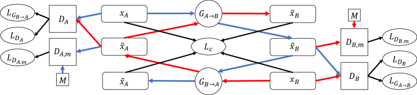
Figure 1: Architecture of our model. The two cycles are shown in blue and red respectively. The black arrows point to the loss functions. We extend the basic CycleGAN architecture with additional discriminators $D_{A,m}$ and $D_{B,m}$.

As in [2], we use the L2 norm for the adversarial loss. For the generators, we have

$$L_{G_{A\rightarrow B}}=\left\|D_{B}\left(\hat{x}_{B}\right)-1\right\|_{2}$$

$$L_{G_{B\rightarrow A}}=\left\|D_{A}\left(\hat{x}_{A}\right)-1\right\|_{2}$$

To enforce forward-backward consistency, Zhu et al. [2] introduce an extra L1 loss term called cycle consistency loss:

$$L_{c}=\left\|\tilde{x}_{A}-x_{A}\right\|_{1}+\left\|\tilde{x}_{B}-x_{B}\right\|_{1}$$

The cycle consistency loss ensures that the input is mapped back to itself after passing it through both generators, i.e., after completing the cycle. If the cycle loss is omitted, the generators will suffer from posterior collapse, and there will only be little or no mutual information between the input and output, which is generally undesirable. The cycle consistency loss can also be seen as a regularizer that makes sure the generators do not ignore the input data, but instead retain as much information as necessary to then be able to invert the transformation.

Thus, the total loss function of the generators is

$$L_{G}=L_{G_{A\rightarrow B}}+L_{G_{B\rightarrow A}}+\lambda L_{c}$$ (1)

Where $\lambda$ is used to weight the contribution of the cycle consistency loss. For the standard GAN discriminators, we have

$$L_{D_{A}}=\frac{1}{2}\left(\left\|D_{A}\left(x_{A}\right)-1\right\|_{2}+\left\|D_{A}\left(\hat{x}_{A}\right)\right\|_{2}\right)$$

$$L_{D_{B}}=\frac{1}{2}\left(\left\|D_{B}\left(x_{B}\right)-1\right\|_{2}+\left\|D_{B}\left(\hat{x}_{B}\right)\right\|_{2}\right)$$

GAN training is highly unstable and the discriminator and generator training needs to be carefully balanced. A common failure mode is when the discriminator is too powerful and overpowers the generator early in training, which results in convergence to a bad local optima. In our setting there is another difficulty: Since the generators need to learn a transformation from a source to a target music genre, they effectively need to learn features of both genres, such that the discriminator can be fooled. It is likely that music genres have a few very distinctive patterns, and that the generators could then simply generate many of these patterns in an attempt to fool the discriminator. Even though the discriminator might be fooled, the output might not sound realistic anymore. In order to force the generators to learn better high-level features, we add two extra discriminators. The main difference to the standard discriminators is that they are trained to distinguish fake data and data from multiple domains ($M$), instead of just data from the target domain. This helps regularize the generator to stay on the “music manifold”, and generate plausible, realistic music. More importantly, it causes the generator to retain much of the input’s structure, thereby ensuring that the original piece is still recognizable after the genre transfer. The loss for these two extra discriminators $D_{A,m}$ and $D_{B,m}$ is

$$L_{D_{A,m}}=\frac{1}{2}\left(\left\|D_{A,m}\left(x_{M}\right)-1\right\|_{2}+\left\|D_{A,m}\left(\hat{x}_{A}\right)\right\|_{2}\right)$$

$$L_{D_{B,m}}=\frac{1}{2}\left(\left\|D_{B,m}\left(x_{M}\right)-1\right\|_{2}+\left\|D_{B,m}\left(\hat{x}_{B}\right)\right\|_{2}\right)$$

where $M$ denotes mixed real data from multiple domains (here possibly Jazz, Classic and/or Pop). Thus the total loss for the discriminators is

$$L_{D,all}=L_{D}+\gamma\left(L_{D_{A,m}}+L_{D_{B,m}}\right)$$ (2)

where $\gamma$ is used to weight the extra discriminator losses. To further stabilize the GAN training we add Gaussian noise $N\left(0,\sigma_{D}^{2}\right)$ to the inputs of the discriminators, similar to [34]. This improves the robustness and generalization performance of the model. The effects of adding the extra discriminators and applying noise to the input of all discriminators are evaluated in Sections VI-B and VI-C.

IV Dataset and Preprocessing

We train our models on music in the MIDI format, which is a symbolic music representation that resembles sheet music. MIDI (Musical Instrument Digital Interface) was originally created as a standard communication interface between electrical instruments, computers and other devices. Thus, MIDI files do not contain actual sound like MP3 files, but instead so-called MIDI messages. For us, the most relevant are the Note On and Note Off messages. The Note On message indicates that a note is beginning to be played, and it also specifies the velocity (loudness) of that note. The Note Off message denotes the end of a note. Each note also has a specified pitch, which in MIDI can range between 0 and 127, corresponding to a note range of $C_{-1}$ to $G_{9}$. A standard piano can play MIDI notes 21 to 108, or equivalently $A_{0}$ to $C_{8}$. Velocity values also range between 0 and 127. Since MIDI files do not contain any sounds themselves, a MIDI synthesizer is required to actually play them. Such synthesizers can either be hardware devices or pieces of software. The final sound will depend on the implementation of the instrument sounds within the used synthesizer.

To input MIDI files to a neural network, they must first be converted into a matrix, the so-called piano roll representation, which can be obtained using the pretty_midi [35] and Pypianoroll [29] Python packages. Since MIDI notes can have arbitrary lengths, it is necessary to re-sample the MIDI file in order to discretize time and allow a matrix representation. We use a sampling rate of 16 time steps per bar, a common choice in the literature ([28, 12]), which means that the shortest possible note is the 16th note. A bar is a segment of time corresponding to a specific number of beats, each of which is represented by a particular note value and the boundaries of the bar are indicated by vertical lines (bars) on a music sheet. For example in the common $\frac{4}{4}$ time signature, a bar contains 4 beats and on each beat we can play a quarter note, two eighth notes, four sixteenth notes, and so on. Thus, our final piano-roll representation is a $t\times p$ matrix, where $t$ denotes the number of time steps (e.g., $t$=16 for a 1-bar piece), and $p$ denotes the number of pitches. We omit the velocity information by setting all velocities to 127, such that every note has the same loudness. This makes learning easier, since every note can now only be on or off, instead of taking 128 possible values. Therefore, the piano-roll representation contains a $p$-dimensional $k$-hot vector at each time step, where $k$ is the number of simultaneously played notes. Because notes with the pitch below C1 or above C8 are not very common, we only retain notes between this range, i.e., $p=84$. Thus, the piano-roll for one bar is of size $16\times 84$. Since music has temporal structures we need to consider the relation of consecutive bars. Therefore, similar to MuseGAN [29], we use phrases consisting of 4 consecutive bars as training samples. Thus, the resulting samples are of size $64\times 84$.

MIDI files can have multiple tracks, where each track can be assigned a different instrument. Since we base our genre transfer solely on note pitches, it is important that we retain as much of the “content” of the original song as possible. Otherwise, the “style” of the song might be lost after selecting only a subset of voices. For example, two songs from two different genres with roughly the same melody but different accompaniments would be difficult to classify if we only consider the notes that comprise the melody. While some previous works select a limited number of voices to make learning easier (e.g.,[12]), we simply merge all notes of all tracks into a single track. By doing so we retain most of the original songs identity, i.e., it is still clearly recognizable as the original song. However, since all notes are now played by the same instrument, the music can sound cluttered. We therefore do not use highly complex pieces of music such as symphonies, as the number of different voices and instruments is simply too high. We further omit the drum track, since it often sounds bad when played by another instrument.

In order to perform domain transfer we require music from different genres. In this paper we use songs from the genres Jazz, Classic and Pop which we collected from various sources. As the dataset is noisy, we need to perform several preprocessing steps. First, we filter out MIDI files whose first beat does not start at 0. Then we remove songs whose time signature changes throughout the song, or whose time signature is not $\frac{4}{4}$. After these preprocessing steps, we have a clean dataset consisting of 12,341 Jazz, 16,545 Classic and 20,780 Pop samples, where the length of one sample is equal to one phrase, or four bars. To avoid introducing a bias due to the imbalance of genres, we reduce the amount of samples in the larger dataset to match that of the smaller one. For example, when training on Jazz and Classic, we randomly sample 12,341 phrases from the Classic dataset to match the size of the Jazz dataset.

V Architecture Parameters and Training

GAN training is generally unstable, as the generator and discriminator need to be carefully balanced. Many techniques have been introduced in order to stabilize GAN training [36], of which we employ several, such as using instance normalization [37] and LeakyReLU [38] activations. During development we experimented with different architectures for the generator and discriminator, before settling on those shown in Tables I and II. The inputs to the generators and discriminators have the shape $\left(batchsize,64,84,1\right)$. Before feeding the samples to the models, we normalize the pitch values to the range [0,1]. We use the Adam [3] optimizer with an initial learning rate of $\alpha=0.0002$. The momentum decay rates are set to $\beta_{1}=0.5$ and $\beta_{2}=0.999$. As suggested by [2], we set $\lambda=10$ in Equation 1. Also, we choose $\gamma=1$ in Equation 2. We train each model for a maximum of 30 epochs, or until the cycle loss converges, and set the batch size to $16$.

TABLE I: Discriminator architecture

Input: $\left(batchsize\times 64\times 84\times 1\right)$
layer	filter	stride	channel	instance norm	activation
conv	$4\times 4$	$2\times 2$	64	False	LReLu
conv	$4\times 4$	$2\times 2$	256	True	LReLu
conv	$1\times 1$	$1\times 1$	1	False	None
Output: $\left(batchsize\times 16\times 21\times 1\right)$

TABLE II: Generator architecture

Input: $\left(batchsize\times 64\times 84\times 1\right)$
layer	filter	stride	channel	instance norm	activation
conv	$7\times 7$	$1\times 1$	64	True	ReLu
conv	$3\times 3$	$2\times 2$	128	True	ReLu
conv	$3\times 3$	$2\times 2$	256	True	ReLu
$10\times$ ResNet	$3\times 3$	$1\times 1$	256	True	ReLu
	$3\times 3$	$1\times 1$	256	True	ReLu
deconv	$3\times 3$	$2\times 2$	128	True	ReLu
deconv	$3\times 3$	$2\times 2$	64	True	ReLu
deconv	$7\times 7$	$1\times 1$	1	False	Sigmoid
Output: $\left(batchsize\times 64\times 84\times 1\right)$

TABLE III: Classifier architecture

Input: $\left(batchsize\times 64\times 84\times 1\right)$
layer	filter	stride	channel	instance norm	activation
conv	$1\times 12$	$1\times 12$	64	False	LReLu
conv	$4\times 1$	$4\times 1$	128	True	LReLu
conv	$2\times 1$	$2\times 1$	256	True	LReLu
conv	$8\times 1$	$8\times 1$	512	True	LReLu
conv	$1\times 7$	$1\times 7$	2	False	Softmax
Output: $\left(batchsize\times 2\right)$

VI Experimental Results

Evaluating the performance of a music generation system is difficult since the goodness of music is a highly subjective measure. Evaluating style and domain transfer is slightly simpler, because one effectively generates aligned pairs of samples, e.g., $x_{A}$ and $\hat{x}_{B}$, where both samples have a domain label. Thus, we can train a style classifier $C_{A,B}$ to distinguish between genre A and B, and then apply it to $x_{A}$ and $\hat{x}_{B}$. If the style transfer works, $C_{A,B}$ will classify $x_{A}$ as $A$, and $\hat{x}_{B}$ as $B$. The more confident the classifier is, the stronger the genre transfer. In the following we describe the style classifier $C_{A,B}$, before describing how the GAN training can be improved by applying Gaussian noise to the discriminator inputs. Finally, we evaluate the style transfer effectiveness of multiple models.

VI-A Genre Classifier

TABLE IV: Average genre classifier accuracy with Gaussian input noise added during testing to evaluate robustness.

$\sigma_{C}$	0	0.01	0.1	0.2	0.3	0.5
Jazz vs. Classic	88.89%	88.53%	87.87%	84.71%	83.07%	74.93%
Classic vs. Pop	84.66%	83.42%	81.97%	81.12%	78.14%	70.28%
Jazz vs. Pop	67.07%	66.18%	63.78%	62.40%	61.72%	59.96%

To evaluate whether our model really learns the translation among different genres, we build a binary classifier $C_{A,B}$ that outputs a probability distribution over domains A and B. The architecture of the genre classifier is shown in Table III. We apply a softmax activation to the two output neurons of the last layer, and optimize the classifier with a cross-entropy loss. We train the genre classifiers on real data from two domains, e.g., Jazz and Classic. The data is the same as that used during the GAN training, and we use a 90/10 train/test split. The performance of the genre classifiers on the test sets is shown in the first column of Table IV. The accuracy on Jazz vs. Classic and Classic vs. Pop is quite high, with 88.89% and 84.66% respectively. The classifier’s performance on Jazz vs. Pop is significantly lower, indicating that the two genres are more similar, at least when only considering note pitches.

The genre classifiers are trained only on real data. However, we want to use them to evaluate whether a domain transfer was successful. For this, we need to apply the classifier on data that has been passed through a generator. If the generator successfully recovered the underlying data generating distribution, the two cases are the same. However, in practice we have to assume that the generator is not perfect and that the generated data that is somehow different from real data. Therefore, the train and test set for the genre classifier effectively come from slightly different distributions, i.e., we are applying the genre classifier on fake data, where during training it has only ever seen real data. This could potentially negatively affect the usefulness of our genre classifier, as we do not know how well it will generalize to fake data. In this paper we investigate the robustness of our genre classifier in the case where the generators apply Gaussian noise to the inputs. This is of course a simplification, since the true transformations applied by the generators are more complex. Table IV shows how the performance of the style classifier changes when Gaussian noise ($\mathcal{N}(0,\sigma_{C}^{2})$) is applied to the inputs of the classifier. Note that the inputs (note pitches) are normalized to lie in the range [-1,1]. The results show that the genre classifier is robust even when adding noise that is large relative to the input value range (i.e. $\mathcal{N}(0,0.5^{2})$). We therefore conclude that the genre classifier learned salient features and cannot easily be broken by random noise. We leave the evaluation of the classifier’s robustness against more sophisticated, possibly even adversarial, noise for future work.

In the following we will use the genre classifier $C_{A,B}$ to evaluate the results of the domain transfer. When considering a transfer from $A$ to $B$, $C_{A,B}$ reports the probability $P_{A}(x)$ if the source genre is $A$, and $P_{B}(x)$ if the source genre is $B$. We consider a domain transfer from $A$ to $B$ as successful if $P_{A}(x_{A})=C_{A,B}(x_{A})>0.5$ AND $P_{A}(\hat{x}_{B})=C_{A,B}(\hat{x}_{B})<0.5$. In other words: If the source style is considered to be more likely before the transfer, and less likely after the transfer. Among the successful domain transfers, we define the strength of the domain transfer in one direction (A $\rightarrow$ B $\rightarrow$ A) as

$$S_{A\rightarrow B}^{D}=\frac{P(A|x_{A})-P(A|\hat{x}_{B})+P(A|\tilde{x}_{A})-P(A|\hat{x}_{B})}{2}$$

For the other direction i.e., (B $\rightarrow$ A $\rightarrow$ B), $S_{B\rightarrow A}^{D}$ is defined analogously. The final domain transfer strength of a particular model is defined as the average of the strengths in both directions

$$S_{tot}^{D}=\frac{1}{2}(S_{B\rightarrow A}^{D}+S_{A\rightarrow B}^{D})$$

The maximum strength that can be achieved is $S_{tot}^{D}=1$ if for both directions, the source style’s probability is equal to 1 before the transfer, equal to 0 after the transfer, and again equal to 1 after completing the cycle. For the remainder of this paper we will use this metric to determine how well a model can perform domain transfer. However, a model that does not retain any structure of the original input can still achieve $S_{tot}^{D}=1$ if the generators learn to perfectly invert each other. Therefore, human judgment is still necessary to determine whether a model performs well. Generally, we are looking for a model that transforms a piece of music from a source to a target genre while retaining as much of the source’s content as possible.

TABLE V: Losses of the base model after 20 epochs. Only for $\sigma_{D}=1$ did the cycle loss converge to 0 and the discriminator and generator are in balance.

$\sigma_{D}$	0	0.01	0.1	1	3	5
$L_{c}$	0.37	0.98	0.20	0.00	0.29	0.87
$L_{G}$	1.20	1.87	1.00	0.52	0.80	1.56
$L_{D}$	0.36	0.27	0.41	0.49	0.50	0.44

VI-B Discriminator Input Noise to Stabilize GAN Training

In order to force the generators and discriminators to learn better features, i.e., avoid overfitting on spurious patterns, and hence improve generalization, we add Gaussian noise $\mathcal{N}(0,\sigma_{D})$ to both real and fake inputs of the discriminators, similar to [34]. We train models for each domain pair with 6 different values for $\sigma_{D}$. For each domain pair and $\sigma_{D}$ value we train three different models: A base model without extra discriminators, a partial model with $D_{A,m}$ and $D_{B,m}$ where $m\in M=A\cup B$ and a full model with $D_{A,m}$ and $D_{B,m}$ where $m\in M=A\cup B\cup C$. Since we have three genres in total, $C$ is always the remaining genre on which none of the base discriminators is trained. For simplicity, we henceforth refer to the three models as $M_{base}$, $M_{partial}$ and $M_{full}$. This results in a total of $3*3*6=54$ models, from which we pick the best ones according to our domain transfer strength metric $S^{D}_{tot}$. For the sake of brevity, we only show the hyper parameter search results for the base model trained on the Jazz and Classic domains. Table V shows the effect of different values for $\sigma_{D}$ on the cycle consistency loss ($L_{c}$), generator loss ($L_{G}$) and discriminator loss ($L_{D}$), respectively. For $\sigma_{D}=1$ the cycle loss converges to zero, and the discriminator and generator losses are balanced, which is generally an indicator that the model converged to a good optima and did not experience a failure mode. Table VI shows the style transfer performance of the same model. According to our genre transfer evaluation metric, the model with $\sigma_{D}=1$ performs best ($S^{D}_{tot}=69.7\%$), which is consistent with the results from Table V. We found that in order to find a model with good performance on a particular domain pair, it is necessary to perform a new parameter search over different values of $\sigma_{D}$.

TABLE VI: Genre transfer performance of the base model measured by a genre classifier with $\sigma_{C}=1$. A contains Jazz pieces and B contains Classic pieces.

$\sigma_{D}$	0	0.01	0.1	1	3	5
A	88.09%	88.09%	88.09%	88.09%	88.09%	88.09%
A$\rightarrow$B	31.38%	5.82%	29.16%	20.62%	12.18%	19.47%
A$\rightarrow$B$\rightarrow$A	84.71%	99.82%	84.36%	88.18%	87.91%	34.13%
B	92.53%	92.53%	92.53%	92.53%	92.53%	92.53%
B$\rightarrow$A	48.80%	56.26%	31.20%	20.71%	61.78%	90.67%
B$\rightarrow$A$\rightarrow$B	89.24%	89.87%	89.33%	92.53%	90.67%	90.67%
$S_{tot}^{D}$	48.5%	61.5%	58.4%	69.7%	52.8%	20.5%

VI-C Genre Transfer

TABLE VII: Genre transfer performance of three different models trained on Jazz and Classic. A: Jazz, B: Classic

	$M_{base}$ $\sigma_{D}=1$	$M_{partial}$ $\sigma_{D}=0$	$M_{full}$ $\sigma_{D}=0.01$
A	88.09%	88.09%	88.09%
A$\rightarrow$B	20.62%	9.87%	20.00%
A$\rightarrow$B$\rightarrow$A	88.18%	87.73%	85.16%
B	92.53%	92.53%	92.53%
B$\rightarrow$A	20.71%	25.87%	20.09%
B$\rightarrow$A$\rightarrow$B	92.53%	89.51%	90.49%
$S_{tot}^{D}$	69.7%	71.6%	69.0%

In this section we evaluate the genre transfer performance of our final models. For each model we indicate the specific value for $\sigma_{D}$ that was used during training. We present domain transfer results on three different domain pairs: Jazz and Classic, Classic and Pop, and Jazz and Pop. For each of these domain pairs we show the results of the models $M_{base}$, $M_{partial}$ and $M_{full}$. Tables VII, VIII and IX show the average genre transfer results of our final models. The tables show the probabilities that the genre classifier $C_{A,B}$ assigned to the source genres. In all cases the transfer is successful, i.e., the genre classifier assigns high probability to the source genre before the transfer, and low probability after the transfer. Please note that since our classifier is binary, a low probability of the source genre is equivalent to a high probability of the target genre. For most models, especially for the Jazz/Classic and Classic/Pop pairs, the genre transfer is very strong, as can be seen from the high values of $S^{D}_{tot}$. For Jazz and Pop, the genre transfer is still successful, but less strong on average. This is due to the fact that the genre classifier $C_{A,B}$ cannot distinguish Pop and Jazz as easily as the other genre pairs.

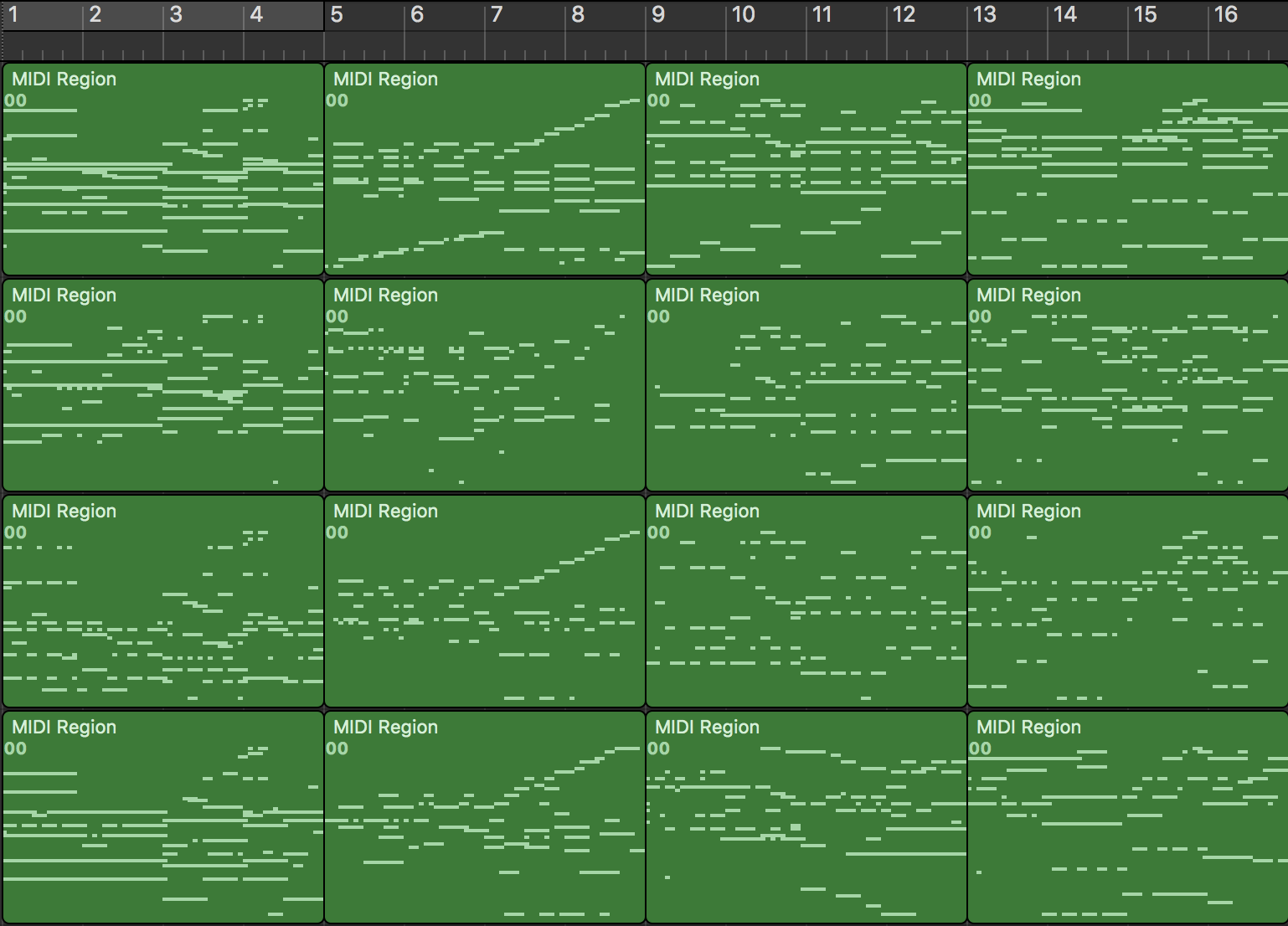
Figure 2: Samples transferred from Jazz to Classic. The first row contains original samples from the test set of domain A (Jazz). The remaining rows show the results from the domain transfer done by models $M_{base}$, $M_{partial}$ and $M_{full}$ respectively (see Table VII for more details on the models).

At first glance, adding the additional discriminators in $M_{partial}$ and $M_{full}$ does not have a clear benefit, at least measured by our domain transfer metric $S^{D}_{tot}$. However, as explained in Section III, adding the additional discriminators encourages the generators to stay on the “music manifold” and has the effect of retaining more of the source’s structure. This can be seen from Figures 2 and 3, where we show some examples for both transfer directions of the Jazz and Classic domain pair. The first row contains four original pieces from the test set. The second row corresponds to the outputs of $M_{base}$, the third row to $M_{partial}$ and the last row to $M_{full}$. $M_{base}$ changes the input too much in most cases, especially when transferring from Classic to Jazz (Figure 3). The differences between $M_{partial}$ and $M_{full}$ are less pronounced, but we find that $M_{full}$ consistently produces better results, i.e., a clearly audible domain transfer while leaving the original melody largely intact. This final evaluation is subjective and we leave the development of better genre transfer metrics for future work. Overall, the genre transfer from Jazz to Classic seems to be most noticeable. Generally, the original songs sound better than the transferred once, indicating that the GAN training needs further improvement to produce better sounding music.

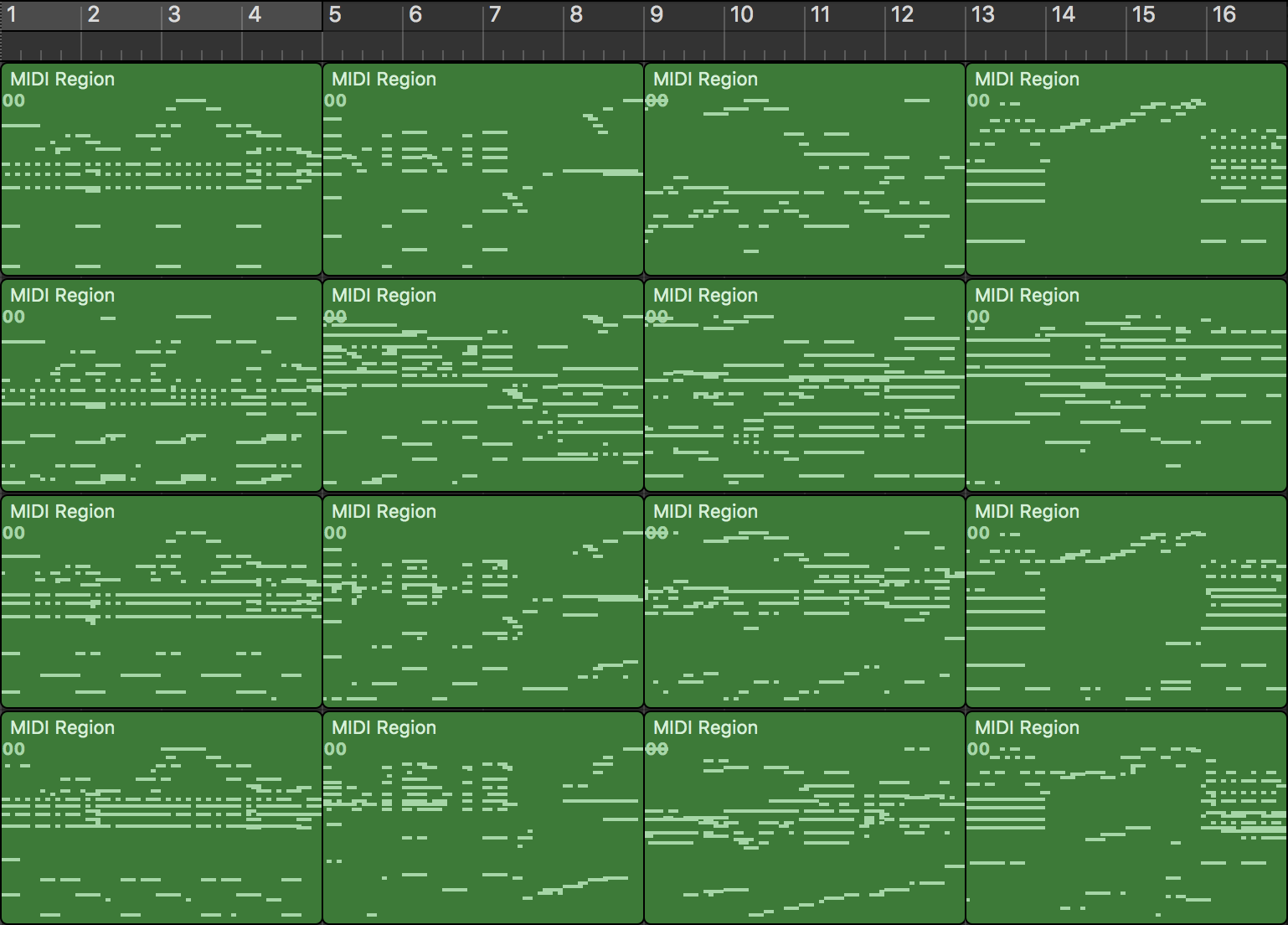
Figure 3: Samples transferred from Classic to Jazz. The first row contains original samples from the test set of domain B (Classic). The remaining rows show the results from the domain transfer done by models $M_{base}$, $M_{partial}$ and $M_{full}$ respectively (see Table VII for more details on the models).

TABLE VIII: Genre transfer performance of three different models trained on Classic and Pop. A: Classic, B: Pop

	$M_{base}$ $\sigma_{D}=0.1$	$M_{partial}$ $\sigma_{D}=1$	$M_{full}$ $\sigma_{D}=1$
A	86.91%	86.91%	86.91%
A$\rightarrow$B	45.12%	38.57%	26.61%
A$\rightarrow$B$\rightarrow$A	83.26%	87.39%	87.18%
B	80.04%	80.04%	80.04%
B$\rightarrow$A	49.14%	23.13%	24.30%
B$\rightarrow$A$\rightarrow$B	72.48%	79.45%	80.15%
$S_{tot}^{D}$	33.6%	52.6%	58.1%

TABLE IX: Genre transfer performance of three different models trained on Jazz and Pop. A: Jazz, B: Pop

	$M_{base}$ $\sigma_{D}=0.01$	$M_{partial}$ $\sigma_{D}=0.01$	$M_{full}$ $\sigma_{D}=0$
A	60.53%	60.53%	60.53%
A$\rightarrow$B	21.60%	14.84%	23.64%
A$\rightarrow$B$\rightarrow$A	57.51%	58.84%	60.53%
B	73.60%	73.60%	73.60%
B$\rightarrow$A	40.62%	43.11%	49.24%
B$\rightarrow$A$\rightarrow$B	74.40%	72.09%	73.06%
$S_{tot}^{D}$	35.4%	37.3%	30.5%

We believe that the results presented in this paper show that GAN-based genre and style transfer for music is a promising direction. In the future we plan to incorporate instrumentation as well as note durations and velocities. Adding these factors, especially instrumentation, should make the genre transfers more easily audible for humans. To complement the presented evaluation, we provide audio samples corresponding to Figures 2 and 3, as well as a few samples of famous songs.

VII Conclusion

In this paper we present, to the best of our knowledge, the first application of GANs to symbolic music domain transfer. We extend the standard CycleGAN model with additional discriminators to regularize the generators. We show that these discriminators improve the generated music by encouraging the generators to preserve the structure of the input, while still performing strong domain transfer. The genre transfer cannot only be picked up by a neural network classifier, but can be heard by the untrained ear. Furthermore, the resulting music has complex structure and generally sounds harmonic. In the future we plan to develop more objective genre transfer metrics, and further investigate the generalization capabilities and robustness of the genre classifier metric. Incorporating richer features such as velocities, note durations and instrumentation could further improve the results and make genre transfers more convincing and realistic. While in this paper we mainly focused on evaluating the basic CycleGAN architecture, more sophisticated architectures should be explored as well.

References

- [1] L. A. Gatys, A. S. Ecker, and M. Bethge, “Image style transfer using convolutional neural networks,” in Computer Vision and Pattern Recognition (CVPR), 2016 IEEE Conference on. IEEE, 2016, pp. 2414–2423.
- [2] J. Zhu, T. Park, P. Isola, and A. A. Efros, “Unpaired image-to-image translation using cycle-consistent adversarial networks,” in IEEE International Conference on Computer Vision, ICCV 2017, Venice, Italy, October 22-29, 2017, 2017, pp. 2242–2251. [Online]. Available: https://doi.org/10.1109/ICCV.2017.244
- [3] D. P. Kingma and M. Welling, “Auto-encoding variational bayes,” CoRR, vol. abs/1312.6114, 2013. [Online]. Available: http://arxiv.org/abs/1312.6114
- [4] I. Goodfellow, J. Pouget-Abadie, M. Mirza, B. Xu, D. Warde-Farley, S. Ozair, A. Courville, and Y. Bengio, “Generative adversarial nets,” in Advances in neural information processing systems, 2014, pp. 2672–2680.
- [5] Y. Bengio, A. C. Courville, and P. Vincent, “Representation learning: A review and new perspectives,” IEEE Trans. Pattern Anal. Mach. Intell., vol. 35, no. 8, pp. 1798–1828, 2013. [Online]. Available: https://doi.org/10.1109/TPAMI.2013.50
- [6] “Bohemian rhapsody for symphony orchestra and solo viola - the studio recording,” https://www.youtube.com/watch?v=aCFnzSCzoYA, accessed: 12-06-2018.
- [7] T. Kaneko and H. Kameoka, “Parallel-data-free voice conversion using cycle-consistent adversarial networks,” CoRR, vol. abs/1711.11293, 2017. [Online]. Available: http://arxiv.org/abs/1711.11293
- [8] Y. Choi, M. Choi, M. Kim, J. Ha, S. Kim, and J. Choo, “StarGAN: Unified generative adversarial networks for multi-domain image-to-image translation,” CoRR, vol. abs/1711.09020, 2017. [Online]. Available: http://arxiv.org/abs/1711.09020
- [9] M. Liu and O. Tuzel, “Coupled generative adversarial networks,” in Advances in Neural Information Processing Systems 29: Annual Conference on Neural Information Processing Systems 2016, December 5-10, 2016, Barcelona, Spain, 2016, pp. 469–477. [Online]. Available: http://papers.nips.cc/paper/6544-coupled-generative-adversarial-networks
- [10] Z. Yi, H. R. Zhang, P. Tan, and M. Gong, “DualGAN: Unsupervised dual learning for image-to-image translation,” in IEEE International Conference on Computer Vision, ICCV 2017, Venice, Italy, October 22-29, 2017, 2017, pp. 2868–2876. [Online]. Available: https://doi.org/10.1109/ICCV.2017.310
- [11] I. Malik and C. H. Ek, “Neural translation of musical style,” CoRR, vol. abs/1708.03535, 2017. [Online]. Available: http://arxiv.org/abs/1708.03535
- [12] G. Brunner, A. Konrad, Y. Wang, and R. Wattenhofer, “MIDI-VAE: Modeling dynamics and instrumentation of music with applications to style transfer,” in Proceedings of the 19th International Society for Music Information Retrieval Conference, ISMIR 2018, Paris, France, September 23-27, 2018, 2018.
- [13] A. van den Oord, O. Vinyals, and K. Kavukcuoglu, “Neural discrete representation learning,” in Advances in Neural Information Processing Systems 30: Annual Conference on Neural Information Processing Systems 2017, 4-9 December 2017, Long Beach, CA, USA, 2017, pp. 6309–6318. [Online]. Available: http://papers.nips.cc/paper/7210-neural-discrete-representation-learning
- [14] N. Mor, L. Wolf, A. Polyak, and Y. Taigman, “A universal music translation network,” CoRR, vol. abs/1805.07848, 2018. [Online]. Available: http://arxiv.org/abs/1805.07848
- [15] A. van den Oord, S. Dieleman, H. Zen, K. Simonyan, O. Vinyals, A. Graves, N. Kalchbrenner, A. W. Senior, and K. Kavukcuoglu, “WaveNet: A generative model for raw audio,” in The 9th ISCA Speech Synthesis Workshop, Sunnyvale, CA, USA, 13-15 September 2016, 2016, p. 125. [Online]. Available: http://www.isca-speech.org/archive/SSW_2016/abstracts/ssw9_DS-4_van_den_Oord.html
- [16] P. M. Todd, “A connectionist approach to algorithmic composition,” Computer Music Journal, vol. 13, no. 4, pp. 27–43, 1989.
- [17] M. C. Mozer, “Neural network music composition by prediction: Exploring the benefits of psychoacoustic constraints and multi-scale processing,” Connect. Sci., vol. 6, no. 2-3, pp. 247–280, 1994. [Online]. Available: https://doi.org/10.1080/09540099408915726
- [18] S. Hochreiter and J. Schmidhuber, “Long short-term memory,” Neural Computation, vol. 9, no. 8, pp. 1735–1780, 1997. [Online]. Available: https://doi.org/10.1162/neco.1997.9.8.1735
- [19] D. Eck and J. Schmidhuber, “A first look at music composition using lstm recurrent neural networks,” Istituto Dalle Molle Di Studi Sull Intelligenza Artificiale, vol. 103, 2002.
- [20] N. Boulanger-Lewandowski, Y. Bengio, and P. Vincent, “Modeling temporal dependencies in high-dimensional sequences: Application to polyphonic music generation and transcription,” in Proceedings of the 29th International Conference on Machine Learning, ICML 2012, Edinburgh, Scotland, UK, June 26 - July 1, 2012, 2012. [Online]. Available: http://icml.cc/2012/papers/590.pdf
- [21] G. Brunner, Y. Wang, R. Wattenhofer, and J. Wiesendanger, “JamBot: Music theory aware chord based generation of polyphonic music with LSTMs,” in 29th International Conference on Tools with Artificial Intelligence (ICTAI), 2017.
- [22] G. Hadjeres, F. Pachet, and F. Nielsen, “DeepBach: a steerable model for bach chorales generation,” in Proceedings of the 34th International Conference on Machine Learning, ICML 2017, Sydney, NSW, Australia, 6-11 August 2017, 2017, pp. 1362–1371. [Online]. Available: http://proceedings.mlr.press/v70/hadjeres17a.html
- [23] H. Chu, R. Urtasun, and S. Fidler, “Song from PI: A musically plausible network for pop music generation,” CoRR, vol. abs/1611.03477, 2016. [Online]. Available: http://arxiv.org/abs/1611.03477
- [24] D. D. Johnson, “Generating polyphonic music using tied parallel networks,” in Computational Intelligence in Music, Sound, Art and Design - 6th International Conference, EvoMUSART 2017, Amsterdam, The Netherlands, April 19-21, 2017, Proceedings, 2017, pp. 128–143. [Online]. Available: https://doi.org/10.1007/978-3-319-55750-2_9
- [25] C.-H. Chuan and D. Herremans, “Modeling temporal tonal relations in polyphonic music through deep networks with a novel image-based representation,” 2018.
- [26] A. Roberts, J. Engel, and D. Eck, “Hierarchical variational autoencoders for music,” in NIPS Workshop on Machine Learning for Creativity and Design, 2017.
- [27] O. Mogren, “C-RNN-GAN: continuous recurrent neural networks with adversarial training,” CoRR, vol. abs/1611.09904, 2016. [Online]. Available: http://arxiv.org/abs/1611.09904
- [28] L. Yang, S. Chou, and Y. Yang, “MidiNet: A convolutional generative adversarial network for symbolic-domain music generation,” in Proceedings of the 18th International Society for Music Information Retrieval Conference, ISMIR 2017, Suzhou, China, October 23-27, 2017, 2017, pp. 324–331. [Online]. Available: https://ismir2017.smcnus.org/wp-content/uploads/2017/10/226_Paper.pdf
- [29] H. Dong, W. Hsiao, L. Yang, and Y. Yang, “MuseGAN: Multi-track sequential generative adversarial networks for symbolic music generation and accompaniment,” in Proceedings of the Thirty-Second AAAI Conference on Artificial Intelligence, New Orleans, Louisiana, USA, February 2-7, 2018, 2018. [Online]. Available: https://www.aaai.org/ocs/index.php/AAAI/AAAI18/paper/view/17286
- [30] L. Yu, W. Zhang, J. Wang, and Y. Yu, “SeqGAN: Sequence generative adversarial nets with policy gradient,” in Proceedings of the Thirty-First AAAI Conference on Artificial Intelligence, February 4-9, 2017, San Francisco, California, USA., 2017, pp. 2852–2858. [Online]. Available: http://aaai.org/ocs/index.php/AAAI/AAAI17/paper/view/14344
- [31] J. D. Fernández and F. J. Vico, “AI methods in algorithmic composition: A comprehensive survey,” J. Artif. Intell. Res., vol. 48, pp. 513–582, 2013. [Online]. Available: https://doi.org/10.1613/jair.3908
- [32] J.-P. Briot, G. Hadjeres, and F. Pachet, “Deep learning techniques for music generation-a survey,” arXiv preprint arXiv:1709.01620, 2017.
- [33] D. Herremans, C. Chuan, and E. Chew, “A functional taxonomy of music generation systems,” ACM Comput. Surv., vol. 50, no. 5, pp. 69:1–69:30, 2017. [Online]. Available: http://doi.acm.org/10.1145/3108242
- [34] C. K. Sønderby, J. Caballero, L. Theis, W. Shi, and F. Huszár, “Amortised MAP inference for image super-resolution,” CoRR, vol. abs/1610.04490, 2016. [Online]. Available: http://arxiv.org/abs/1610.04490
- [35] M. Data, “Intuitive analysis, creation and manipulation of midi data with pretty_midi,” 2014.
- [36] “How to train a GAN? tips and tricks to make GANs work,” https://github.com/soumith/ganhacks, accessed: 12-06-2018.
- [37] D. Ulyanov, A. Vedaldi, and V. S. Lempitsky, “Instance normalization: The missing ingredient for fast stylization,” CoRR, vol. abs/1607.08022, 2016. [Online]. Available: http://arxiv.org/abs/1607.08022
- [38] A. L. Maas, A. Y. Hannun, and A. Y. Ng, “Rectifier nonlinearities improve neural network acoustic models.”