Taylor dispersion in two-dimensional bacterial turbulence

Abstract

In this work, single particle dispersion was analyzed for a bacterial turbulence by retrieving the virtual Lagrangian trajectory via numerical integration of the Lagrangian equation. High-order displacement functions were calculated for cases with and without mean velocity effect. Two-regime power-law behavior for short and long time evolutions were identified experimentally, which were separated by the Lagrangian integral time. For the case with the mean velocity effect, the experimental Hurst numbers were determined to be $0.94$ and $0.97$ for short and long times evolutions, respectively. For the case without the mean velocity effect, the values were $0.88$ and $0.58$. Moreover, very weak intermittency correction was detected. All measured Hurst number were above $1/2$, the value of the normal diffusion, which verifies the super-diffusion behavior of living fluid. This behavior increases the efficiency of bacteria to obtain food.

I Introduction

A bacterial suspension in a thin fluid can be approximated as a 2D fluid system when the considered spatial scale is larger than the fluid depth. In this active system, the energy injection and dissipation patterns are quite peculiar. Considering classical three-dimensional homogeneous and isotropic turbulence, the energy is transferred from large-scale to small-scale structures until the viscosity scale, where the kinetic energy dissipates as heat.(Frisch, 1995) In the bacterial turbulence, the kinetic energy is injected into the system via a scale of the bacterial body length $R$, which is typically around a few $\mu$m, and then transfers from small-scale to large-scale ones via an inverse cascade process.Wensink et al. (2012) The velocity of the bacterial turbulence is also on the order of a few $\mu$m per second, and the Reynolds number is nearly zero. Due to hydrodynamic interactions, the bacterial flow exhibits turbulent-like features, such as, long range correlation and power-law of the spectrum.(Wu and Libchaber, 2000; Pooley, Alexander, and Yeomans, 2007; Ishikawa et al., 2011; Wensink et al., 2012; Dunkel et al., 2013; Marchetti et al., 2013; Bratanov, Jenko, and Frey, 2015; Qiu et al., 2016) For instance, Wensink et al. (2012) observed a dual-power-law behavior in a quasi-2D active fluid, which was separated by the viscosity-like scale at $\ell=10R$. Qiu et al. (2016) confirmed the intermittency correction, one of the most important features of the turbulence, directly via a Hilbert-based methodology. They found a dual-power-law behavior, which is separated by a viscosity-like scale $\ell_{\nu}\simeq 10R$. The scaling behavior below the viscosity scale $\ell_{\nu}$ is more intermittent than the behavior above the scale $\ell_{\nu}$. This bacterial or active turbulence is now named as “mesoscale turbulence”.(Wensink et al., 2012; Bratanov, Jenko, and Frey, 2015)

Note that there is no commonly accepted unique definition of turbulent flow: it is usually identified by its main features that a broad range of spatial and temporal scales or many degrees of freedom are excited in the system.(Groisman and Steinberg, 2000) Another “narrow definition” of turbulence has been proposed by Gibson (2004) that “turbulence is defined as an eddy-like state of fluid motion where the inertial vortex forces of the eddies are larger than any other forces that tend to dampen the eddies out.” Rotational turbulent eddies form at the viscosity scale (resp. Kolmogorov scale), and then they pair with neighboring ones, and these new pairs pair with neighboring pairs, and so on to generate large-scale structures.(Gibson, 2004) This is indeed the idea of the inverse energy cascade. It seems that this definition of turbulence is applicable to the bacterial turbulence aforementioned. More discussions and examples of this “narrow definition of turbulence” can be found in Ref. (Gibson, 2004) and Ref. .

Single particle dispersion in disordered or turbulent flow in classical turbulence and living fluid is still fundamentally unclear. LaCasce (2008); Bechinger et al. (2016) In single particle dispersion, also known as Taylor dispersion, the mean square displacement, $\mathcal{D}_{2}(\tau)$, is defined as,

$$\mathcal{D}_{2}(\tau)=\langle r_{i}(t,\tau)^{2}\rangle_{i,t}$$ (1)

where $r_{i}(t,\tau)=|\mathbf{x}_{i}(t,+\tau)-\mathbf{x}_{i}(t)|$ is the displacement function; $\mathbf{x}_{i}(t)$ is a Lagrangian trajectory; and $\tau$ is the separation time scale. According to the Taylor dispersion theory, the following two regimes are expected,

$$\mathcal{D}_{2}(\tau)=\left\{\begin{array}[]{lll}&\tilde{v}^{2}\tau^{2},&\textrm{when }\tau\ll T_{L}\\ &2\tilde{v}^{2}T_{L}\tau,&\textrm{when }\tau\gg T_{L}\end{array}\right.$$ (2)

where $T_{L}$ is the Lagrangian integral time scale; and $\tilde{v}^{2}$ is the variance of Lagrangian velocity.(Taylor, 1921; Bouchaud and Georges, 1990) The latter scaling regime is also known as normal diffusion. Metzler and Klafter (2000); Vlahos and Isliker (2008) Experimentally, the measured scaling exponent of Eq. (LABEL:eq:Taylor), $\mathcal{D}_{2}(\tau)\propto\tau^{\gamma_{2}}$, might be different with the above mentioned values. For example, Wu and Libchaber (2000) studied the collective dynamics of bacteria in a freely suspended soap film via the Lagrangian particle tracking technique. They found that the measured mean displacement function of beads demonstrates a super-diffusion (resp. $\gamma_{2}>1$) in short-time period and normal diffusion (resp. $\gamma_{2}\simeq 1$) in long-time period. Xia et al. (2014) performed an experimental particle tracking study in a traditional two-dimensional turbulence system. Based on the measured scaling exponent, $\gamma_{2}$, a transition phenomenon of $\gamma_{2}$ from $2$ (super-diffusion) to $1$ (normal diffusion) was observed as the Reynolds number increased. Based on this observation, a so-called fully developed two-dimensional turbulence was defined. Ariel et al. (2015) tracked the trajectory of individually fluorescently labeled bacteria within such dense swarms. The authors reported a super-diffusion behavior with a measured scaling exponent $\gamma_{2}\simeq 1.6$, which can be further described and modeled by the Lévy walk. Note that for the bacterial case, the diffusion or dispersion behavior is highly dependent on many factors, such as the concentration of the bacteria, temperature and chemical gradients.

In this work, virtual particles were tracked using a numerical integration of the Lagrangian equation based on measurements of the Eulerian velocity field of bacterial turbulence via particle image velocimetry.Jullien, Paret, and Tabeling (1999) The dispersion of the particles was calculated, and the results show a clear two-regime behavior, which is separated by the Lagrangian integral time. Despite the numerical value of the scaling exponent, $\gamma_{2}$, the Taylor dispersion theory is evident from the obtained results. The possible intermittent correction was also checked experimentally by generalization of the mean square displacement function to the $q$th order, e.g., $\mathcal{D}_{q}(\tau)=\langle r_{i}(t,\tau)^{q}\rangle_{i,t}$.

II experimental data

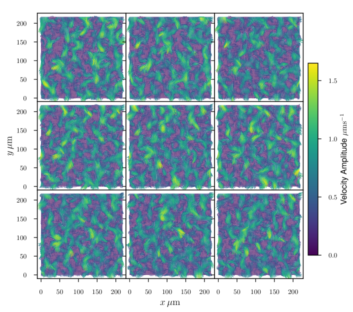
Figure 1: (Color online) Illustration of nine successive snapshots of instantaneous velocity vector, where the velocity amplitude is coded in color. A typical vortex structure with spatial size of $\sim 50\,\mathrm{\mu m}$ is observed.

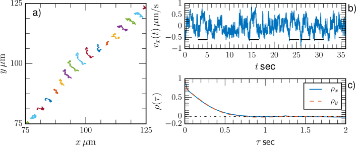
Figure 2: (Color online) a) Illustration of Lagrangian trajectories. b) The Lagrangian velocity $v_{x}$ along the trajectory. The horizontal solid line indicates a time span $2\,$\mathrm{s}\mathrm{e}\mathrm{c}$$. c) Experimental autocorrelation function $\rho(\tau)$ for Lagrangian velocities $v_{x}$ and $v_{y}$. The corresponding zero-crossing based Lagrangian time is $\sim 0.75\,$s.

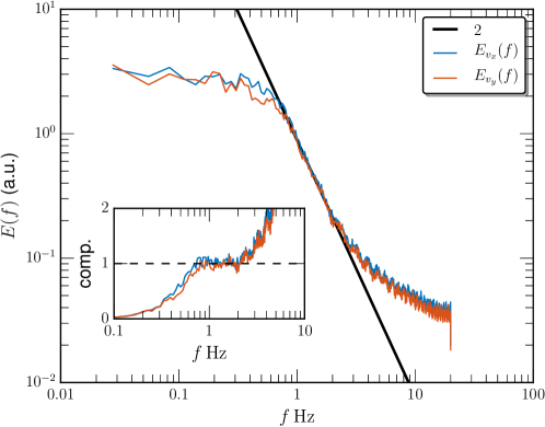
Figure 3: (Color online) Fourier power spectrum of Lagrangian velocities of ${v_{x}}$ and ${v_{y}}$. Power-law behavior is observed in the frequency range $0.6\leq f\leq 2\,$Hz with a scaling exponent $2.0\pm 0.06$, which is in agreement with the value predicted by the Kolmogorov-Landau theory for the conventional Lagrangian turbulence. The inset shows a compensated curve to emphasize the observed scaling range.

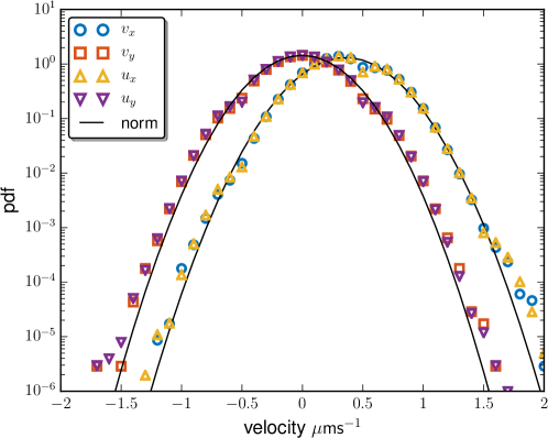
Figure 4: (Color online) Probability density function of Eulerian ($\mathbf{u}$) and Lagrangian velocity ($\mathbf{v}$), where normal distribution is illustrated by the solid line.

II.1 Experimental Setup

The experimental data analyzed here was provided by Professor Raymond E. Goldstein at the Cambridge University, UK. We briefly recall the main parameters of this quasi-2D experiment in a microfluidic chamber. The bacteria used in this experiment was B. subtilis with individual body lengths of approximately $5\,\mu$m, in which the energy is injected into the system. The volume filling fraction was $\phi=84\%$ with particle number $N=9968$ and aspect ratio $a=5$ (the ratio between the bacterial body length $R$ and the body diameter). The quasi-2D microfluidic chamber had a vertical height, $H_{c}$, less than or equal to the individual body length of B. subtilis (approximately 5$\,\mu$m). With these parameters, the flow entered a turbulent phase.Wensink et al. (2012) The particle image velocimetry (PIV) had a measurement area of $217\mathrm{\mu m}\times 217\mathrm{\mu m}$. The image resolution was $700\,$pix$\times 700\,$pix with a conversion rate of $0.31\,\mathrm{\mu m}/$pix and a frame rate of $40\,$Hz. The commercial PIV software Dantec Flow Manager was used to extract the flow field component with a moving window size of $32\,$pix$\times 32\,$pix and $75\%$ overlap. This resulted in an $84\times 84$ velocity vector and a total of 1441 snapshots, corresponding to a period of $\sim 36\,$seconds. Therefore, a spatial structure size $\ell$ larger than $H_{c}$ can be treated as a two-dimensional system. The mean and root-mean-square (rms.) velocities were determined to be $\overline{\mathbf{u}}=(0.36,0)\,\mathrm{\mu ms^{-1}}$ and $\mathbf{u}^{{}^{\prime}}=(0.30,0.29)\,\mathrm{\mu ms^{-1}}$, respectively, and the corresponding turbulent intensity was around $\mathbf{u}^{\prime}/\overline{\mathbf{u}}_{x}\simeq 82\%$. The PIV uncertainty was less than $1\%$ for the second-order statistics. More details of this database can be found in Ref. Wensink et al., 2012.

Figure 1 shows nine successive snapshots of the instantaneous velocity vector, where the velocity amplitude is coded in color. A typical flow structure with a spatial size around $\sim 50\,\mathrm{\mu m}$ is visually evident and has been recognized as a fluid-viscosity-like scale.Qiu et al. (2016) The flow is smooth in space due to fluctuations in the high wave number (for structures smaller than $50\,\mathrm{\mu m}$) that will be quickly damped by the viscosity.

II.2 Numerical Tracking Algorithm

Using the measured Eulerian velocity field, $\mathbf{u}(\mathbf{x},t)$, we numerically integrated the Lagrangian equation as follows,

$$\frac{\mathrm{\,d}\mathbf{x}}{\mathrm{\,d}t}=\mathbf{v}(\mathbf{x},t)$$ (3)

where $\mathbf{v}(\mathbf{x},t)$ is the Lagrangian velocity; and $\mathbf{v}(\mathbf{x},t)$ is equal to the Eulerian velocity at the same position, e.g., $\mathbf{v}(\mathbf{x},t)=\mathbf{u}(\mathbf{x},t)$. A second-order Adams-Bashforth method was employed in the time scheme, while a two-dimensional spline interpolation scheme was used to retrieve the Lagrangian velocity not on the grid point. The virtual particles were assumed to be free with the bacteria body, or in other words, they could freely penetrate the bacteria body. Initially, $2500$ virtual fluid particles were seeded with a uniform distribution in the range $(x,y)\in[0,217]\,\mathrm{\mu m}$. If a particle moved beyond the experimental area, time integration stopped. For one realization, about $\sim$100 virtual particles exceeded the boundary, and ten realizations were performed. In totally, we obtained $2400\times 1441\times 10\simeq 34,584,000$ (number of virtual particles per realization $\times$ number of snapshots $\times$ number of realizations) velocity vectors to ensure a good statistics.

Figure 2 a) illustrates several trajectories that show a complex behavior. Figure 2 b) shows the Lagrangian velocity $v_{x}(t)$ along the Lagrangian trajectory, where a large structure fluctuation is visible around $\sim 2\,$\mathrm{s}\mathrm{e}\mathrm{c}$$. From there, we estimated the Lagrangian velocity correlation function as,

$$\rho(\tau)=\frac{\langle\tilde{v}(t+\tau)\tilde{v}(t)\rangle_{t}}{\sigma^{2}}$$ (4)

where $\tilde{v}(t)=v(t)-\langle v(t)\rangle_{t}$ is a centered Lagrangian velocity; $\langle\,\rangle_{t}$ is time average; and $\sigma$ is the root-mean-square Lagrangian velocity. Figure 2 c) displays the experimental $\rho(\tau)$ for $v_{x}(t)$ and $v_{y}(t)$, which show long range correlation in time. The Lagrangian time scale, $T_{L}$, is defined as,

$$T_{L}=\int_{0}^{\infty}\rho(\tau)\mathrm{\,d}\tau$$ (5)

Due to the finite time measurement, it is difficult to apply the above definition directly. Therefore, we used the first zero-crossing time as the Lagrangian integral time, i.e., $T_{L}=\tau_{0}$, where $\rho(\tau_{0})=0$. The experimental value of $T_{L}$ is found to be $\sim 0.75\,\mathrm{sec}$; thus we expect two dispersion regimes to be separated by the Lagrangian time scale, $T_{L}$.

Figure 3 shows the measured Fourier power spectrum for the Lagrangian velocities $v_{x}$ and $v_{y}$. Power-law behavior, $E(f)\sim f^{-\beta}$, was observed in the range $0.6\leq f\leq 2\,\mathrm{Hz}$, corresponding to the time scale range $0.5\leq t\leq 1.7\,\mathrm{sec}$. A compensated curve using the measured scaling exponent is also shown in the inset in Fig. 3 to emphasize the power-law behavior, where a clear plateau confirms the existence of the power-law behavior. The measured scaling exponent is $\beta=2.0\pm 0.06$, where the error is provided by the $95\%$ fitting confidence level of the least square fit algorithm. This scaling value is coincidently in a good agreement with the value predicted by the Kolmogorov-Landau theory for hydrodynamical Lagrangian turbulence.Falkovich et al. (2012); Huang et al. (2013) Note that, due to the existence of vortex trapping events in the conventional three-dimensional Lagrangian turbulence, this value is difficult to obtain even turbulent flows with high Reynolds numbers.Falkovich et al. (2012)

Figure 4 shows the measured probability density function (pdf) of Eulerian velocity, $\mathbf{u}$, and Lagrangian velocity, $\mathbf{v}$, where the normal distribution is represented by a solid line. As seen in the figure, the measured pdfs of Eulerian and Lagrangian velocities agree well with the normal distribution.Wensink et al. (2012)

III Results

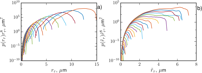
Figure 5: (Color online) Convergence test of $8$th-order displacement function $\mathcal{D}_{8}(\tau)=\int p(r_{\tau})r_{\tau}^{8}\mathrm{\,d}r_{\tau}$, where $p(r_{\tau})$ is the experimental pdf of the displacement function with the separation time scale $\tau$. The corresponding integral kernel: a) with mean velocity effect, and b) without mean velocity effect. It confirms the statistical convergence for all separation scales at least up to the statistical order $q=8$.

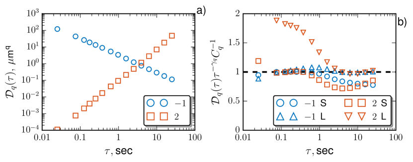
Figure 6: (Color online) a) Measured $q$th-order displacement function $\mathcal{D}_{q}(\tau)$ for statistical order $q=-1$ ($\ocircle$) and $2$ ($\square$). b) The compensated curve to emphasize the power-law behavior in the range $0.05\leq\tau\leq 0.5\,$sec and $2\leq\tau\leq 31\,$sec using measured scaling exponents $\gamma_{2}^{S}=1.87\pm 0.01$ and $\gamma^{L}_{2}=1.93\pm 0.01$, respectively, and the corresponding fitting constant, $C_{q}$.

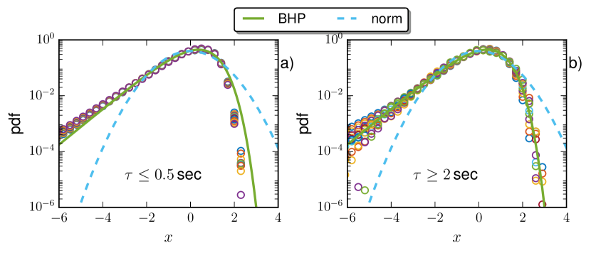
Figure 7: (Color online) Experimental pdf of the centered $x$, where $x=(x_{\tau}-\langle x_{\tau}\rangle)/\sigma$ and $x_{\tau}=\log_{10}(r(\tau))$ for a) $\tau\leq 0.5\,$sec and b) $\tau\geq 2\,$sec. For comparison, the Bramwell-Holdsworth-Pinton formula (thick solid line) and the normal distribution (dashed line) are also shown.

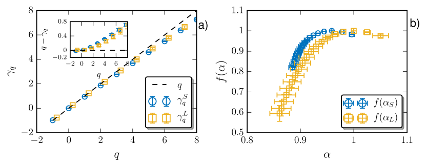
Figure 8: (Color online) a) Measured scaling exponents, $\gamma_{q}$, for short and long time evolutions. For comparison, the scaling $\gamma_{q}=q$ is represented by a dashed line. The inset shows the deviation from the linear relation $\gamma_{q}=q$. b) The corresponding singularity spectrum, $f(\alpha)$, versus $\alpha$. The error is provided by the $95\%$ fitting confidence level.

III.1 Convergence test

To analyze the convergence of statistics in this work, we first considered the $q$th-order displacement function, which is defined as,

$$\mathcal{D}_{q}(\tau)=\langle r_{i}(t+\tau)^{q}\rangle_{i,t}$$ (6)

which can be re-written as,

$$\mathcal{D}_{q}(\tau)=\int_{0}^{\infty}p(r_{\tau})r_{\tau}^{q}\mathrm{\,d}r_{\tau}$$ (7)

where $p(r_{\tau})$ is the experimental pdf for the separation time scale, $\tau$; and $p(r_{\tau})r_{\tau}^{q}$ is the so-called $q$th-order integral-kernel. Figure 5 shows the measured integral-kernels for a) with and b) without the mean velocity effect by removing the persistent velocity effect from the displacement function, i.e., $\tilde{r}_{i}(\tau)=|\mathbf{x}_{i}(t+\tau)-\mathbf{x}_{i}(t)-V\tau|$, where $V=\langle v(t)\rangle_{t}$ is the mean Lagrangian velocity. Visually, the measured curve initially increased and then curved downward, which indicates a good convergence of the statistics at least up to the statistical order $q=8$. We then considered the statistics in the range $-1\leq q\leq 8$ and time scale in the range $0.05\leq\tau\leq 31\,$sec.

III.2 Taylor dispersion with mean velocity effect

Figure 6 a) shows the experimental $q$th-order displacement function for $q=-1$ ($\ocircle$) and $q=2$ ($\square$). The power-law behavior is evident, as expected, and can be further identified by two regimes, e.g., $0.05\leq\tau\leq 0.5\,$sec, and $2\leq\tau\leq 31\,$sec, which are separated by the above estimated Lagrangian time scale, $T_{L}=0.75\,\mathrm{sec}$. Figure 6 b) displays the corresponding compensated curve using the fitted scaling exponent, $\gamma_{2}$, to emphasize the observed power-law behavior, in which a clear plateau confirms the existence of the power-law behavior. The measured scaling exponents for the case $q=2$ were determined to be $\gamma^{S}_{2}=1.87\pm 0.01$ and $\gamma_{2}^{L}=1.93\pm 0.01$, where the error is provided by the $95\%$ fitting confidence level. The former value is close to the value $\gamma_{2}=2$, which was predicted by the Taylor dispersion theory for a short time evolution. Due to the existence of the mean velocity effect, the latter scaling exponent is also close to $2$.

Experimental pdfs for the normalized displacement functions, $x=(x_{\tau}-\langle x_{\tau}\rangle)/\sigma$ and $x_{\tau}=\log_{10}(r(\tau))$, were calculated with a bin width of $0.1$. Figure 7 shows the measured pdfs for a) $\tau\leq 0.5\,$sec and b) $\tau\geq 2\,$sec. Except for slight scattering at the right ($x\geq 1$) and left ($x\leq-4$) tails, they collapsed with each other on their own regimes, indicating the scale invariance property. For comparison, the normal distribution and the Bramwell-Holdsworth-Pinton (BHP) formula,(Bramwell, Holdsworth, and Pinton, 1998) are displayed as dashed and solid lines, respectively. The BHP formula is written as

$$\Pi(y)=K(e^{y-e^{y}})^{a},\,y=b(x-s),a=\pi/2,$$ (8)

where parameters $b=0.938$, and $K=2.14$ were obtained numerically from a previous study. (Bramwell et al., 2000) This formula was first introduced to characterize rare fluctuations in turbulence and critical phenomena. The measured pdfs for small-scale separation time ($\tau\leq 0.5\,$sec) agrees with the BHP formula on the range $-4\leq x\leq 0.6$. For large-scale separation time ($\tau\leq 2\,$sec), the pdfs agree well with the BHP when $x\geq-4$.

We then estimated the scaling exponents on these two scaling regimes for $-1\leq q\leq 8$. Figure 8 a) shows the measured scaling exponents, $\gamma_{q}$, for both short ($\ocircle$) and long time ($\square$) evolutions, where $\gamma_{q}=q$ predicted by the Taylor dispersion theory for short time evolutions is shown as a dashed line. The error bar indicates a $95\%$ fitting confidence interval. Experimentally, the measured scaling exponents, $\gamma^{S}_{q}$ and $\gamma^{L}_{q}$, are close to each other since the mean Lagrangian velocity effect is preserved in the numerical integral algorithm, but deviate from the prediction of the Taylor dispersion theory (inset of Fig. 8 a). A nonlinear $q$-dependence of these curves implies a potential intermittency correction. To characterize the potential intermittency effect, we introduce here a lognormal formula to fit the measured scaling exponents, which is written as,

$$\gamma(q)=qH-\frac{\mu}{2}\left(q^{2}H^{2}-qH\right)$$ (9)

where $H$ is the Hurst number and $\mu$ is the intermittency parameter. (Li and Huang, 2014) This lognormal formula is a generalization of the classical one proposed by Kolmogorov in 1960s for the hydrodynamic turbulence with $H=1/3$. For a given $H$, a larger value of $\mu$ is, a more intermittenter process. The measured parameters $H_{S}=0.94\pm 0.01$ and $\mu_{S}=0.01\pm 0.001$, and $H_{L}=0.97\pm 0.01$ and $\mu_{L}=0.02\pm 0.001$ show a very weak intermittent correction, where the error is provided by the $95\%$ fitting confidence level.

Note that for the lognormal formula, both $H$ and $\mu$ are taken as free parameters. The measured intermittency parameter, $\mu$, depends on $H$. To overcome this difficulty, we introduce here a singularity spectrum, which is defined via a Legendre transform,

$$f(\alpha)=\min_{q}\{q\alpha-\gamma_{q}+1\},\quad\alpha(q)=\frac{\mathrm{\,d}\gamma_{q}}{\mathrm{\,d}q}$$ (10)

where $\alpha$ is the multifractal intensity; and $f(\alpha)$ is the singularity spectrum. Experimentally, a wider $\alpha$ and $f(\alpha)$ refer to a more intermittent field. Figure 8 b) shows the measured $f(\alpha)$ versus $\alpha$, where a weak intermittent correction exists for both small and large time scales. Moreover, the singularity spectrum for large-scale time separations seems to be more intermittent than that for small-scale one.

III.3 Taylor dispersion without mean velocity effect

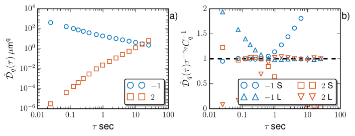
Figure 9: (Color online) a) Measured $q$th-order mean displacement function, $\tilde{\mathcal{D}}_{q}(\tau)$, for statistical order $q=-1$ ($\ocircle$) and $2$ ($\square$) without mean velocity effect. b) The compensated curve to emphasize the power-law behavior in the ranges $0.05\leq\tau\leq 0.5\,$sec and $2\leq\tau\leq 31\,$sec.

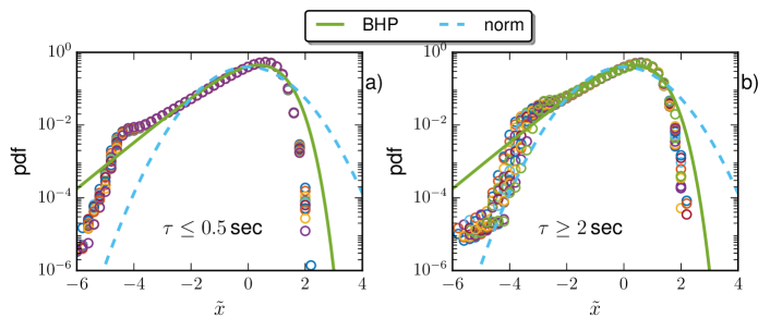
Figure 10: (Color online) Experimental normalized pdfs of the centered displacement $\tilde{x}$, where $\tilde{x}=(\tilde{x}_{\tau}-\langle\tilde{x}_{\tau}\rangle)/\sigma$ and $\tilde{x}_{\tau}=\log_{10}(\tilde{r}(\tau))$ for a) $\tau\leq 0.5\,$sec and b) $\tau\geq 2\,$sec. For comparison, the BHP formula and the normal distribution are also shown.

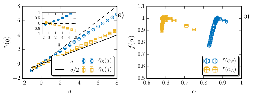
Figure 11: (Color online) a) Measured scaling exponents $\tilde{\gamma}_{q}$ for short and long time evolutions without mean velocity effect. For comparison, the scaling $\tilde{\gamma}_{q}=q$ and $\tilde{\gamma}_{q}=q/2$ are illustrated as dashed and solid lines. b) The corresponding singularity spectrum, $f(\alpha)$, versus $\alpha$.

To exclude the mean velocity effect, a displacement function that omits this effect is defined as,

$$\mathcal{\tilde{D}}_{q}(\tau)=\langle\tilde{r}_{i}(t+\tau)^{q}\rangle_{i,t}$$ (11)

where $\tilde{r}_{i}(t+\tau)=|\mathbf{x}_{i}(t+\tau)-\mathbf{x}_{i}(t)-V\tau|$; and $V=\langle v(t)\rangle_{t}$ is the mean Lagrangian velocity. This formula represents a dispersion observed on a moving frame with a constant velocity, $V$. Figure 9 a) shows the measured $\tilde{\mathcal{D}}_{q}(\tau)$ for statistical order $q=-1$ ($\ocircle$) and $q=2$ ($\square$). Power-law behavior is observed with two different regimes in the time ranges $0.05\leq\tau\leq 0.5\,$sec and $2\leq\tau\leq 31\,$sec with scaling exponents $\tilde{\gamma}^{S}_{2}=1.74\pm 0.02$ and $\tilde{\gamma}^{L}_{2}=1.16\pm 0.01$, where the error is provided by the $95\%$ fitting confidence level. The former scaling exponent is smaller than the one predicted by the Taylor dispersion theory for short time evolutions, and is similar to the one reported by Ariel et al. (2015). The latter scaling exponent for long time evolutions is slight larger than the value of $1$, indicating a super-diffusion. This result reveals the effects of bacterial turbulence. The compensated curve is shown in Fig. 9 b) to emphasize the power-law behavior. A clear plateau confirms the existence of the power-law.

Figure 10 shows the experimental pdfs $p(\tilde{x})$ of $\tilde{x}=(\tilde{x}_{\tau}-\langle\tilde{x}_{\tau}\rangle)/\sigma$ and $\tilde{x}_{\tau}=\log_{10}(\tilde{r}(\tau))$ for a) $0.05\leq\tau\leq 0.5\,$sec and b) $2\leq\tau\leq 31\,$sec. Visually, these differ greatly from the pdfs obtained with the BHP formula or normal distribution. Moreover, we discovered that the pdfs for small (resp. $0.05\leq\tau\leq 0.5\,$sec) and large (resp. $2\leq\tau\leq 31\,$sec) times collapse with each other when $-4\leq x$. The collapse implies that, if the intermittency correction exists, their strengths could be the same for these two different regimes.

Figure 11 a) shows the measured scaling exponents, $\tilde{\gamma}_{q}$, for both small ($\ocircle$) and large ($\square$) time evolutions. For comparison, values predicted by Taylor dispersion theory are also shown. Visually, the scaling exponent $\tilde{\gamma}_{q}^{S}$ in short time evolutions is below the theoretical one when $q\geq 0$, while the expnoent in long time evolution is above the theoretical one when $q\geq 0$, indicating super-diffusion. The corresponding deviation from the theoretical values are shown in the inset in Fig.11 a). Note that these curves are almost linear against $q$, indicating that the possible intermittency correction is possibly negligible. The lognormal formula fitting provides $\tilde{H}_{S}=0.88\pm 0.01$ and $\tilde{\mu}_{S}=0.01\pm 0.001$, and $\tilde{H}_{L}=0.58\pm 0.01$ and $\tilde{\mu}_{L}=-0.01\pm 0.005$, where the error is provided by the $95\%$ fitting confidence level. These values suggest a very weak intermittency correction, confirming the observations from Fig. 11 a). Figure 11 b) shows the measured singularity spectrum, $f(\alpha)$, versus $\alpha$ where the intermittency correction could be ignored for both short and long time evolutions.

IV Discussion

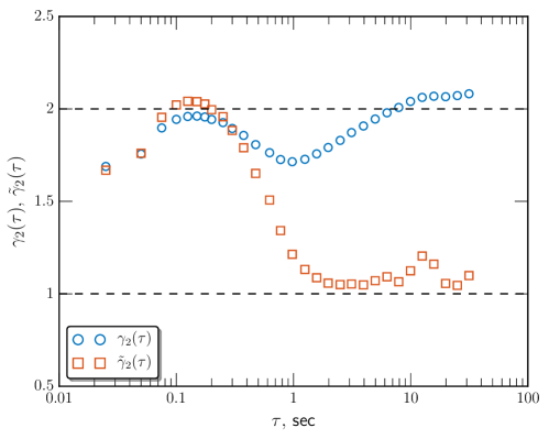
Figure 12: (Color online) Experimental local scaling exponent $\gamma_{2}(\tau)$ (resp. $\tilde{\gamma}_{2}(\tau)$) for the mean square displacement for $\mathcal{D}_{2}(\tau)$ (resp. $\mathcal{\tilde{D}}_{2}(\tau)$). The lack of a plateau implies the absence of a pure power-law behavior.

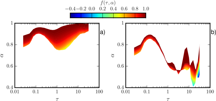
Figure 13: (Color online) Experimental local singularity spectrum, $f(\tau,\alpha)$, a) with and b) without mean velocity effect. For comparison convenience, measured $f(\tau,\alpha)$ is coded by the same color map.

The measured scaling exponents, $\gamma_{q}$, may vary for different fitting ranges. This is because that a pure power-law behavior is difficult to retrieve, and this can be seen from a local scaling exponent, $\gamma_{2}(\tau)$, which is defined as,

$$\gamma_{2}(\tau)=\frac{\mathrm{\,d}\log_{10}\mathcal{D}_{2}(\tau)}{\mathrm{\,d}\log_{10}\tau}$$ (12)

This exponent can be generalized for a $q$th-order displacement function $\mathcal{D}_{q}(\tau)$. Figure 12 shows the measured $\gamma_{2}(\tau)$ (resp. $\tilde{\gamma}_{2}(\tau)$), where the lack of a clear plateau implies the absence of pure power-law behavior. In other words, the experimental scaling exponent, $\gamma_{2}$, might depend on the choice of the fitting range. To avoid this vagueness, we introduce here a local singularity spectrum,

$$f(\tau,\alpha)=\min_{q}\left\{q\alpha(\tau,q)-\gamma_{q}(\tau)+1\right\},\,\alpha(\tau,q)=\frac{\mathrm{\,d}\gamma_{q}(\tau)}{\mathrm{\,d}q}$$ (13)

where $\alpha(\tau,q)$ is the local multifractal intensity; and $f(\tau,\alpha)$ is the local singularity spectrum. Figure 13 shows a contour plot of the measured local singularity spectrum $f(\tau,\alpha)$ respectively for a) with and b) without the mean velocity effect. For visual convenience, the plots are coded in the same color map. Visually, two different regimes are visible with either a small variation of $\alpha(\tau,q)$ or $f(\tau,\alpha)$, indicating that the intermittency correction is very weak if it exists. This is consistent with the direct measurement of the intermittency parameter, $\mu\simeq 0.01$.

The measured Hurst number, $H$, either with or without mean velocity effect are different than the ones predicted by the Taylor dispersion theory. This difference may be an effect of the active movement of bacteria, which are aided by super-diffusion to capture food.(Ariel et al., 2015) Although the two regimes are experimentally evident, this result is a consequence of the turbulent motion of such bacterial turbulent flow.

Finally, we would like to provide some comments on the statistical uncertainty of this study. As mentioned above, the statistical uncertainty of the PIV measurement is less than $1\%$ for the second-order moment.(Wensink et al., 2012) We have tested for different algorithms for both time advance and spatial interpolation, and found that the individual trajectories starting from the same initial positions vary slightly. However, the statistical moments of displacement functions are the same, which is partially due to a rather smooth fluid field. Further, the displacement function, $\mathcal{D}_{q}(\tau)$, is indeed a structure-function of the Lagrangian trajectory. Therefore, $V_{\tau}=\mathcal{D}_{1}(\tau)/\tau$ can be treated as a coarse-grained mean velocity, which is less influenced by the intermittency effect that has been found for the Eulerian velocity field.(Qiu et al., 2016) We also note that some velocity vectors from 10 realizations are not statistically independent. But it does not change the conclusion of this work. However, a true particle tracking experiment should be done with carefully designed as a means to directly check the dispersion relations.

V Conclusion

In summary, single particle dispersion was analyzed for a bacterial turbulence by numerical integration of the Lagrangian equation. A second-order Adams-Bashforth scheme in time and a two-dimensional spline interpolation scheme in space were used, and $q$th-order displacement functions with and without the mean velocity effect were calculated. The results show a two-regime behavior respectively in short and long time evolutions with corresponding regimes in the range $0.05\leq\tau\leq 0.5\,$sec and $2\leq\tau\leq 31\,$sec, respectively. With the mean velocity effect, the experimental pdfs of the displacement function was fitted via the BHP formula, and the measured scaling exponents, $\gamma_{q}$, was found to deviate from the one predicted by the Taylor dispersion theory, which can be understood as an effect of the active dynamic system. Moreover, the corresponding Hurst numbers were determined to be $H_{S}=0.94$ and $H_{L}=0.97$. When excluding the mean velocity effect, the measured pdfs of displacement function collapse with each other and were different from the BHP formula, while the measured scaling exponents, $\gamma_{q}$, deviated from the theoretical prediction. More precisely, in short time evolutions ($0.05\leq\tau\leq 0.5\,$sec), the measured Hurst number was $\tilde{H}_{S}=0.88$, smaller than the value of the theoretical prediction. In long time evolutions ($2\leq\tau\leq 31\,$sec), the measured Hurst number was $\tilde{H}_{L}=0.58$ and is larger than the value predicted by the Taylor dispersion theory. All these measured Hurst numbers indicate a super-diffusion behavior, which is relevant for bacteria to gain food more efficiently. Furthermore, the experimental results show a weak intermittency effect. Excluding the results obtained for the Hurst numbers, the two-regime behavior predicted by the Taylor dispersion theory is verified for this active turbulence system.