Tight Continuous-Time Reachtubes for Lagrangian Reachability

Abstract

We introduce continuous Lagrangian reachability (CLRT), a new algorithm for the computation of a tight and continuous-time reachtube for the solution flows of a nonlinear, time-variant dynamical system. CLRT employs finite strain theory to determine the deformation of the solution set from time $t_{i}$ to time $t_{i+1}$. We have developed simple explicit analytic formulas for the optimal metric for this deformation; this is superior to prior work, which used semi-definite programming. CLRT also uses infinitesimal strain theory to derive an optimal time increment $h_{i}$ between $t_{i}$ and $t_{i+1}$, nonlinear optimization to minimally bloat (i.e., using a minimal radius) the state set at time $t_{i}$ such that it includes all the states of the solution flow in the interval $[t_{i},t_{i+1}]$. We use $\delta$-satisfiability to ensure the correctness of the bloating. Our results on a series of benchmarks show that CLRT performs favorably compared to state-of-the-art tools such as CAPD in terms of the continuous reachtube volumes they compute.

I Introduction

Recent work introduced Lagrangian ReachTube algorithm (LRT), a new approach for the reachability analysis of continuous, nonlinear, dynamical systems [8]. LRT constructs a discrete-time reachtube (or flowpipe) that given a dynamical system, tightly overestimates the set of reachable states at each time point.

The main idea of LRT was to construct a ball-overestimate in a metric space that minimizes the Cauchy-Green stretching factor at every discrete time instant. LRT was shown to compare favorably to other reachability analysis tools, such as CAPD [5, 27] and Flow* [6, 7] in terms of the discrete reachtube volumes they compute on a set of well-known benchmarks.

This paper proposes a continuous-time-reachtube extension of LRT, the motivation for which is two-fold. First, LRT, while being optimal in the discrete setting, is not sound in the continuous setting: it is not obvious how to find a ball tightly overestimating the dynamics between two discrete points. Second, LRT is not directly applicable to the analysis of hybrid systems, as the dynamics of a hybrid system may change dramatically between two discrete time points due to a mode switch.

The main goal of our algorithm, which we call continuous Lagrangian ReachTube algorithm (CLRT), is to efficiently construct an ellipsoidal continuous-reachtube overestimate that is tighter than those constructed by available state-of-the-art tools such as CAPD. CLRT combines a number of techniques to achieve its goal, including infinitesimal strain theory, analytic formulas for the tightest deformation metric, nonconvex optimization, and $\delta$-satisfiability. Computing an as tight-as-possible Lagrangian continuous-reachtube overestimate helps avoid false positives when checking if a set of unsafe states can be reached from a set of initial states.

The class of continuous dynamical systems in which we are interested is described by nonlinear, time-variant, ordinary differential equations (ODEs):

$$\dot{x}(t) =f(t,x(t)),$$ (1a)

$$x(t_{0}) =x_{0},$$ (1b)

where $x\colon\mathbb{R}\to\mathbb{R}^{n}$. We assume $f$ is a smooth function, which guarantees short-term existence of solutions. The class of time-variant systems strictly includes the class of time-invariant systems.

Given an initial time $t_{0}$, set of initial states $\mathcal{X}\subset\mathbb{R}^{n}$, and time bound $T\,{>}\,t_{0}$, CLRT computes a conservative reachtube of (1), that is, a sequence of time-stamped sets of states $(R_{1},t_{1}),{\dots},(R_{k},t_{k}=T)$ satisfying:

$$\text{Reach}\left((t_{0},\mathcal{X}\right),[t_{i-1},t_{i}])\subset R_{i}\text{ for }i=1,\dots,k,$$

where $\text{Reach}\left((t_{0},\mathcal{X}\right),[t_{i-1},t_{i}])$ denotes the set of all reachable states of ODE system (1) in the time interval $[t_{i-1},t_{i}]$. The time steps are not necessarily uniformly spaced, and are chosen using infinitesimal strain theory (IST).

In contrast to LRT [8], which only computes the set of states reachable at discrete and uniformly spaced time steps $t_{i}$, for $i\,{\in}\,\{1,{\ldots},k\}$, CLRT computes a tight overestimate for the set of states reachable in non-uniformly spaced continuous time intervals $[t_{i-1},t_{i}]$. Hence, CLRT computes space-time cylinders overestimating the continuous-time reachtube.

We also note that the LRT approach, as in prior work on reachability [12, 17], employed semi-definite programming (SDP) to compute an appropriate weighted norm minimizing the Cauchy-Green stretching factor (deformation metric). We instead derive a very simple analytic formula for the tightest deformation metric. Thus, there is no need to invoke an optimization procedure to find a tight deformation metric, as the formula for the tightest one is now available. We also provide a very concise proof of this fact. Moreover, using SDP significantly increases the running time of the algorithm (compared to the approach based on analytical formulas), and can result in numerical instabilities (refer to the discussion in [8]) and excessive bloating.

Let us enumerate the key contributions of this work; 1. Computation of tightest Lagrangian reachtubes using explicit analytic formulas for the deformation metric. 2. Derivation of continuous-time reachtube bounds by bloating the discrete-time reachtube via nonconvex optimization. 3. Application of infinitesimal strain theory to adaptive time-step selection. 4. Computation of the stretching factor is derived in weighted metric spaces, where the natural enclosures are ellipsoids. 5. Demonstrate improved performance by using ellipsoidal bounds in place of boxes, which are more natural for control theoretic verification problems.

Let $\text{Reach}\left((t_{0},\mathcal{X}\right),t_{i-1})\,{\subset}\,B_{M_{i-1}}(x_{i-1},\delta_{i-1})$, where $B_{M_{i-1}}(x_{i-1},\delta_{i-1})$ is the ball computed by LRT for time $t_{i-1}$. To construct a continuous reachtube overestimate for the interval $[t_{i-1},t_{i}]$, we bloat the radius of this ball to $\Delta_{i-1}\,{>}\,\delta_{i-1}$, until it becomes a tight overestimate for the entire interval; i.e., $\text{Reach}\left((t_{0},\mathcal{X}\right),[t_{i-1},t_{i}])\,{\subset}\,B_{M_{i-1}}(x_{i-1},\Delta_{i-1})$.

To ensure that the bloating is as tight as possible, we first find the largest time $t_{i}$ such that the displacement gradient tensor of the solutions originating in $B_{M_{i-1}}(x_{i-1},\delta_{i-1})$ becomes sufficiently close to linear. Second, to obtain an initial estimate $\hat{\Delta}_{i-1}$, we assume that $f$ in (1) is convex in the interval $[t_{i-1},t_{i}]$, and solve a convex optimization problem. Third, because for general nonlinear systems $f$ is likely non-convex, we, through an iterative process where $\hat{\Delta}_{i-1}$ is used as an initial value, compute a sound estimate of $\Delta_{i-1}$ using an SMT solver.

We have implemented a prototype of CLRT in C++ and thoroughly investigated its performance on a set of benchmarks, including those used in [8]. Our results show that compared to CAPD, CLRT performs favorably in terms of the continuous-reachtube volumes they compute. Also note that contrary to LRT, CLRT is fully implemented in C++, which significantly improves the runtime performance of our algorithm. Presently, CLRT externally uses CAPD to compute gradients of the flow, but we know how to achieve this independently, and we are currently working on implementing/distributing CLRT as a software library written in C++.

The rest of the paper is organized as follows. Section II provides background on infinitesimal strain theory, LRT, and convex optimization. Sections IV and V describe the bloating factor and optimization steps that we use. Section VI presents the CLRT algorithm. Section VII contains our experimental results. Section IX offers our concluding remarks and directions for future work.

II Background

This section gives the necessary background, such that paper is self contained. We present techniques that are used by the CLRT algorithms presented in Section VI to construct overestimating tight continuous reachtubes.

II-A Finite and Infinitesimal Strain Theory

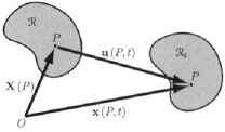
Figure 1: The reference (or initial) configuration $\mathcal{R}$ and the current configuration $\mathcal{R}_{t}$ of a body $\mathbb{B}$ subjected to deformation [26]. A material point $P$ has reference coordinates $\mathbf{X}(P)$ in $\mathcal{R}$, and current coordinates $\mathbf{x}(P,t)$ in $\mathcal{R}_{t}$, if one uses the same system of coordinates. The displacement vector $u$ shows how the position of a material point $P$ changes from $\mathcal{R}$ to $\mathcal{R}_{t}$.

A central assumption in continuum mechanics is that a body can be modeled as a continuum, and that the physical quantities distributed over the body can be therefore represented by continuous fields [26].

A body $\mathbb{B}$ is composed of an infinite number of material points $P$ and the assignment of each of these material points to a unique position in space defines a configuration of $\mathbb{B}$. A reference (or initial) configuration of $\mathbb{B}$ occupying region $\mathcal{R}$ is used for comparison with the current configurations of $\mathbb{B}$ occupying region $\mathcal{R}_{t}$ at subsequent moments of time $t$.

Given a material point $P\,{\in}\,\mathbb{B}$, the position vector $\mathbf{X}(P)$ of $P$ relative to a prescribed origin $O$ in $\mathcal{R}$ is called $P$’s reference position. The position vector $\mathbf{x}(P,t)$ of $P$ relative to $O$ in $\mathcal{R}_{t}$ is called the current position of $P$. For simplicity, Figure 1 uses the same coordinate systems for $\mathcal{R}$ and $\mathcal{R}_{t}$. However, as we show later, it is convenient to use different coordinate systems or vector bases, which minimize the associated norms of $\mathcal{R}$ and $\mathcal{R}_{t}$. The coordinates of the reference (undeformed) $\mathcal{R}$ are called Lagrangian, whereas the ones of the current (deformed) $\mathcal{R}_{t}$ are called Eulerian.

The displacement $\mathbf{u}$ of a material point $P$ from its position in $\mathcal{R}$ to its position in $\mathcal{R}_{t}$ is defined by the following vector equation:

$$\mathbf{u}(P,t)=\mathbf{x}(P,t)-\mathbf{X}(P)$$ (2)

Assuming that each material point $P$ in $\mathbb{B}$ occupies a single position in space at time $t$, there is a (nonlinear) vector operator $\mathbf{\chi}$, mapping $\mathbf{X}(P)$ to $\mathbf{x}(P,t)$, that is, $\mathbf{x}(P,t)\,{=}\,\mathbf{\chi}(\mathbf{X}(P),t)$. Using $\mathbf{\chi}$, the Lagrangian description of the displacement field is given by the following equation:

$$\mathbf{u}=\mathbf{\chi}(\mathbf{X(P)},t)\,{-}\,\mathbf{X}(P)$$ (3)

A tensor $\mathbf{T}(P,t)$ is a physical quantity associated with the material point $P$ of a body $\mathbb{B}$ at the time $t$. This representation can be given in either Lagrangian coordinates as $\mathbf{T}(P,t)\,{=}\,\mathbf{\Psi}(\mathbf{X}(P),t)$ or Eulerian coordinates as $\mathbf{T}(P,t)\,{=}\,\mathbf{\psi}(\mathbf{x}(P,t),t)$. Since the tensor is the same no matter in which coordinates it is expressed, the Lagrangian description is related to the Eulerian description by:

$$\mathbf{\Psi}(\mathbf{X}(P),t)\,{=}\,\mathbf{\psi}(\mathbf{\chi}(\mathbf{X}(P),t),t)$$ (4)

A particularly important (nonsingular) tensor is the deformation gradient tensor $\mathbf{F}$ defined by the following equation:

$$\mathbf{F}=\nabla_{X}\,\mathbf{x}(P,t)=\nabla_{X}\,\mathbf{\chi}(\mathbf{X}(P),t)$$ (5)

By Equations (2,3), the displacement gradient tensor is related to the deformation gradient tensor as follows:

$$\nabla_{X}\,\mathbf{u}=\mathbf{F}-\mathbf{I}$$ (6)

where $I$ is the identity matrix. A description of the deformation independent of both translation and rotation is given by a strain tensor, of which the right Cauchy-Green deformation tensor $\mathbf{C}$ and the Green-St. Venant strain tensor $\mathbf{E}$, are two examples:

$$\mathbf{C}=\mathbf{F}^{T}\cdot\mathbf{F}\qquad\mathbf{E}=(\mathbf{C}-\mathbf{I})/2$$ (7)

Now by using the definition of $\mathbf{F}$ from Equation 6, the Green-St. Venant strain tensor $\mathbf{E}$ can be rewritten as follows:

$$\mathbf{E}=[(\nabla_{X}\,\mathbf{u})+(\nabla_{X}\,\mathbf{u})^{T}+(\nabla_{X}\,\mathbf{u})^{T}\cdot(\nabla_{X}\,\mathbf{u})]/2$$ (8)

If the norm $\|\nabla_{X}\,\mathbf{u}\|\,{\ll}\,1$, that is, each component of $\nabla_{X}\,\mathbf{u}$ is of order $O(\varphi)$, for some small parameter $\varphi$, then one speaks about infinitesimal deformation and the associated theory is called the infinitesimal strain theory (IST).

In this case, the product $(\nabla_{X}\,\mathbf{u})^{T}\cdot(\nabla_{X}\,\mathbf{u})$ is of order $O(\varphi^{2})$, and it can be therefore neglected. This, leads to the linearized version $\mathbf{\varepsilon}$ of $\mathbf{E}$:

$$\mathbf{\varepsilon}=[(\nabla_{X}\,\mathbf{u})+(\nabla_{X}\,\mathbf{u})^{T}]/2$$ (9)

which is called the infinitesimal strain tensor $\mathbf{\varepsilon}$. Similarly, the infinitesimal rotation tensor $\mathbf{\omega}$ is defined as follows:

$$\mathbf{\omega}=[(\nabla_{X}\,\mathbf{u})-(\nabla_{X}\,\mathbf{u})^{T}]/2$$ (10)

For infinitesimal deformations, $d\mathbf{X}\,{=}\,d\mathbf{x}$, and for any tensor $\mathbf{T}$, the gradients of $\mathbf{T}$ with respect to the Lagrangian and Eulerian coordinates are the same, as $\delta\mathbf{T}/\delta{X}\,{=}\,\delta\mathbf{T}/\delta{x}$ [26]. Hence, in IST it is not necessary to distinguish anymore between Lagrangian and Eulerian coordinates.

II-B Review of the LRT Algorithm

The LRT algorithm computes a conservative, discrete-time reachtube for nonlinear, time-variant dynamical systems, based on finite strain theory [8].

The main idea of LRT is to use the right Cauchy-Green strain tensor $\mathbf{C}$ to determine, in a tightest metric, the stretching factor (SF) of a ball propagated by the system dynamics in the next time step. According to Eqs. (6,7), $\mathbf{C}\,{=}\,\mathbf{F}^{T}\cdot\mathbf{F}$,  $\mathbf{F}\,{=}\,\nabla_{X}\,\mathbf{x}$, and $\mathbf{x}\,{=}\,\mathbf{\chi}(\mathbf{X},t)$, where $\mathbf{\chi}(\mathbf{X},t)$ is the solution-flow of the system. $\mathbf{F}$ is the sensitivity matrix [9].

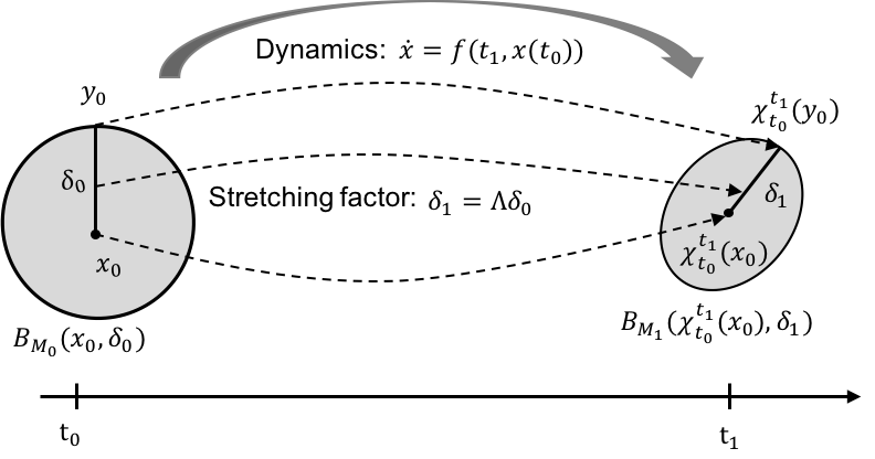
Figure 2: Overview of LRT from [8]. Dashed arrows reflect the solution flow $\chi$ and the evolution of state discrepancy.

By $\|\cdot\|_{2}$ we denote the Euclidean norm, by $\|\cdot\|_{\infty}$ we denote the max norm; we use the same notation for the induced operator norms; We use the standard notation $\succ 0$ for positive definiteness. Let $B(x,\delta)$ be the closed ball centered at $x$ with radius $\delta$. $B_{M}(x,\delta)$ is the closed ball in the metric space defined by matrix $M\succ 0$. By $\chi_{t_{0}}^{t_{1}}$ we denote the flow induced by (1). $\nabla_{x}\chi_{t_{0}}^{t_{1}}$ denotes the partial derivative in $x$ of the flow WRT the initial condition at time $t_{1}$, which we call the gradient of the flow, also referred to as the sensitivity matrix [9, 10]. Let $M\in\mathbb{R}^{n\times n}$ and $M\succ 0$. We say that matrix $M$ defines a metric space when the metric of this space is defined using the distance function $d_{M}(x,y)=\sqrt{x^{T}My}$. We denote the norm weighted by $M\succ 0$ as $\|x\|_{M}=\sqrt{x^{T}Mx}$.

Let matrices $M_{0},M_{1}\succ 0$ define two metric spaces. Let $B_{M_{0}}(x_{0},\delta_{0})$ be an initial region, given as a ball in metric space $M_{0}$, centered at $x_{0}$ and of radius $\delta_{0}$. Let $y_{0}$ be a point on the surface of $B_{M_{0}}(x_{0},\delta_{0})$, and $x^{\prime}_{0}\,{=}\,\mathbf{\chi}_{t_{0}}^{t_{1}}(x_{0})$ and $y^{\prime}_{0}\,{=}\,\mathbf{\chi}_{t_{0}}^{t_{1}}(y_{0})$, where $\mathbf{\chi}_{t_{0}}^{t_{1}}(x)$ abbreviates the solution flow $\mathbf{\chi}(x,t_{0},t_{1})$ of $x$ when time passes from $t_{0}$ to $t_{1}$. Let $\delta_{1}$ be the distance between $y^{\prime}_{0}$ and $x^{\prime}_{0}$ in the metric space defined by matrix $M_{1}$ (see Figure 2 for a geometric representation).

SF $\Lambda$ measures the deformation of the ball $B_{M_{0}}(x_{0},\delta_{0})$ into the ball $B_{M_{1}}(x^{\prime}_{0},\delta_{1})$, i.e. $\Lambda\,{=}\,\delta_{1}{/}\delta_{0}$. One can thus use the SF to bound the infinite set of reachable states at time $t_{1}$ with the ball-overestimate $B_{M_{1}}(\chi_{t_{0}}^{t_{1}}(x_{0}),\delta_{1})$ in an appropriate metric $M_{1}\succ 0$, which may differ from $M_{0}\succ 0$. If $M_{1}\,{=}\,M_{0}$ we refer to the computed SF as $M_{0}$-SF or $M_{1}$-SF, and if $M_{0}\neq M_{1}$ we refer to the computed SF as $M_{0,1}$-SF.

LRT’s performance on computing tighter overapproximation depends on an appropriate choice of matrix $M_{1}$. LRT computes $M_{1}\,{\succ}\,0$ by solving a semi-definite optimization problem. Note that the output produced by LRT can be used to compute a validated bound for the finite-time Lyapunov exponent (FTLE) $\ln(\Lambda){/}T$, where $T$ is the time horizon. FTLE is used e.g, in climate research to detect Lagrangian-coherent structures [23]. The correctness of the LRT algorithm is given by the following theorem [8].

Theorem 1 (Thm. 1 in [8])

Let $t_{0}\,{\leq}\,t_{1}$ be time points, and $\chi_{t_{0}}^{t_{1}}(x)$ the solution at $t_{1}$ of the Cauchy problem (1), with initial condition $(t_{0},x)$. Let $M_{0},M_{1}\in\mathbb{R}^{n\times n}$ with $M_{0},M_{1}\,{\succ}\,0$, and $A_{0}^{T}A_{0}=M_{0}$, $A_{1}^{T}A_{1}=M_{1}$ their respective decompositions. Let the ball in the $M_{0}$-norm with center $x_{0}$ and radius $\delta_{0}$, $\mathcal{X}=B_{M_{0}}(x_{0},\delta_{0})\subseteq\mathbb{R}^{n}$ be a set of initial states for (1). Assume that there exists a compact, conservative enclosure $\mathcal{F}\subseteq\mathbb{R}^{n\times n}$ for the gradients such that:

$$\nabla_{x}\chi_{t_{0}}^{t_{1}}(x)\in\mathcal{F},\quad\forall x\in\mathcal{X}.$$ (11)

Suppose $\Lambda\,{>}\,0$ is an upper bound of the whole set of $M_{0,1}$ SFs [8], that is:

$$\Lambda\geq\sqrt{\lambda_{max}\left((A_{0}^{T})^{-1}F^{T}M_{1}FA^{-1}_{0}\right)},\quad\forall F\in\mathcal{F}.$$ (12)

where $\lambda_{max}$ represents the maximum eigenvalue. Then, every solution at time $t_{1}$ belongs to the ball:

$$\chi_{t_{0}}^{t_{1}}(x)\in B_{M_{1}}(\chi_{t_{0}}^{t_{1}}(x_{0}),\Lambda\cdot\delta_{0}).$$ (13)

Observe that ${\sqrt{\lambda_{max}\left((A_{0}^{T})^{-1}F^{T}M_{1}FA^{-1}_{0}\right)}}={\left\|A_{1}FA^{-1}_{0}\right\|_{2}}$, where $\|\cdot\|_{2}$ is spectral (Euclidean) matrix norm.

III Explicit Analytic Computation of the Tightest Deformation Metric

Observe that Thm. 1 provides freedom in switching metric spaces used from step to step (by convention, $M_{0}\succ 0$ denotes the initial metric, and $M_{1}\succ 0$ denotes the metric of the solution-set bound after one time-step). To decide if a change of norm should be performed, we compute $\hat{M}_{1}$ that minimizes the $M_{1}$-stretching factor $\left({\sqrt{\lambda_{max}\left((A_{1}^{T})^{-1}F^{T}M_{1}FA^{-1}_{1}\right)}}\right)$, and decide based on that; i.e., if the resulting $\hat{M}_{1}$-stretching factor (SF) is by some measure significantly smaller than the $M_{0}$-SF $\left({\sqrt{\lambda_{max}\left((A_{0}^{T})^{-1}F^{T}M_{0}FA^{-1}_{0}\right)}}\right)$, then switching to $\hat{M}_{1}$ may result in a tighter overestimate.

We provide here a surprising argument that the optimal choice of $\hat{M}_{1}$ minimizing the $M_{1}$-SF, as well as its decomposition $\hat{M}_{1}=\hat{A}_{1}^{T}\hat{A}_{1}$ can be obtained using a straightforward computation that we present here.

Motivated by related work [12, 17], the LRT approach [8] identified a tight metric by solving a Semi-Definite Programming (SDP) problem. We show that we do not need to invoke any (convex) optimization technique to find a tight deformation metric, because actually there exist explicit simple analytical formulas for the tightest deformation metric. In particular, this improves upon existing results two-fold: the computation is much faster, and the computed bounds are tighter than the ones computed using SDP. We provide an illustrative example to support our claims in Fig. 3. We are convinced that our technique can be applied in the related settings considered in [12, 17], where the authors compute continuous reach-tubes by overestimating solution flows using matrix measures.

Our goal is to minimize the value of $\Lambda$, the upper bound for the $M_{1}$-SF given in Theorem 1. As finding the best enclosure for a set of SF is a hard problem, we use the following heuristics. The set of gradients $\mathcal{F}\subset\mathbb{R}^{n\times n}$ in our algorithm is given by an interval matrix. Our choice of $M_{1}$ is determined by the value of the gradient $F$ being the middle of $\mathcal{F}$, i.e. $F=\operatorname{mid}{(\mathcal{F})}$. We derive an analytical formula for $\hat{M}_{1}$ minimizing the $M_{1}$-SF for $F$. We devote the remainder of this section to answer the following crucial question.

For a given gradient matrix $F$, what is the $\hat{M}_{1}$ minimizing the $M_{1}$ SF?

Definition 1 (Analytic $\hat{M}_{1}\succ 0$)

Let $F\in\mathbb{R}^{n\times n}$ be a full-rank matrix (in our application a gradient of the flow). Let $V(F)\in\mathbb{C}^{n\times n}$ denote the invertible matrix of normalized eigenvectors of $F$ (column-wise). To make this matrix invertible in the case of higher-dimensional eigenspaces (where some eigenvectors are equal), we need to include generalized eigenvectors. For gradients of nonlinear flow equal eigenvectors rarely occurs; hence we do not treat the case of equal eigenvalues in detail.

We define $\hat{M}_{1}$ as follows:

$$\hat{A}_{1}(F)=V(F)^{-1}\quad\text{and}\quad\hat{M}_{1}(F)=\hat{A}_{1}(F)^{T}\hat{A}_{1}(F)$$ (14)

When $F$ is known from context, we simply write
$\hat{A}_{1}=\hat{A}_{1}(F)\text{, and }\hat{M}=\hat{M}_{1}(F)$.

We now prove that the choice made in Def. 1 is optimal, i.e. it minimizes the $M_{1}$ SF. We remark that our choice of $\hat{M_{1}}$ is unique by construction using normalized eigenvectors.

Theorem 2 ($\hat{M}_{1}$ is optimal)

Let $F\in\mathbb{R}^{n\times n}$ be a full-rank matrix. Let $\hat{A}_{1}$ and $\hat{M}_{1}$ be defined by (14). Let the $M_{1}$-SF be given by

$$\Lambda(A_{1},F)={\sqrt{\lambda_{max}\left((A_{1}^{T})^{-1}F^{T}M_{1}FA^{-1}_{1}\right)}}={\left\|A_{1}FA^{-1}_{1}\right\|_{2}}$$

It holds that

$$\min_{\begin{subarray}{c}A_{1}\in\mathbb{R}^{n\times n}\\ A_{1}\text{ is invertible}\end{subarray}}{\Lambda(A_{1},F)}=\Lambda(\hat{A}_{1},F),$$

i.e., $\hat{M}_{1}=\hat{A}_{1}^{T}\hat{A}_{1}$ minimizes the $M_{1}$-SF.

Proof:

First, for arbitrary $A_{1}$, it holds that

$$\sigma_{1}(A_{1}FA^{-1}_{1})=\|A_{1}FA^{-1}_{1}\|_{2}=\max_{\|x\|=1,\|y\|=1}{\left|y^{T}A_{1}FA^{-1}_{1}x\right|},$$

where $\sigma_{1}$ denotes the largest singular value of $A_{1}FA^{-1}_{1}$.

Let us pick $y^{T}=w^{T}$, and $x=w$, where $w$ is the normalized eigenvector corresponding to the largest eigenvalue of $A_{1}FA^{-1}_{1}$. We have

$$\|A_{1}FA^{-1}_{1}\|_{2}=\max_{\|x\|_{2}=1,\|y\|_{2}=1}{\left|y^{T}A_{1}FA^{-1}_{1}x\right|}\geq\\ \left|w^{T}A_{1}FA^{-1}_{1}w\right|=|\lambda_{max}(A_{1}FA^{-1}_{1})|=|\lambda_{max}(F)|.$$

Hence, the $M_{1}$ SF cannot be smaller than $|\lambda_{max}(F)|$.

Second, we show that this lower bound is in fact attained for $\hat{A}_{1}=\hat{A}_{1}(F)$ defined by (14). We have

$$\|\hat{A}_{1}F\hat{A}_{1}^{-1}\|_{2}=\sqrt{\lambda_{max}\left((\hat{A}_{1}^{T})^{-1}F^{T}\hat{A}_{1}^{T}\hat{A}_{1}F\hat{A}_{1}^{-1}\right)}\\ =\sqrt{\lambda_{max}\left(\operatorname{diag}(|\lambda_{1}|^{2},\dots,|\lambda_{n}|^{2})\right)}=|\lambda_{max}(F)|,$$

where $\lambda_{1},\dots,\lambda_{n}$ denote the eigenvalues of $F$. ∎

Remark 1

Let us remark on how we compute matrix $\hat{A}_{1}$ in practice. Generally, this matrix is complex, as the gradient of the flow is expected to involve some rotation. We do not work within the field $\mathbb{C}$ as we apply algorithms for bounding eigenvalues of real matrices. Instead, we compute the equivalent real matrix $\hat{A}_{1}$, such that the resulting product $\hat{A}_{1}F\hat{A}_{1}^{-1}$ is block-diagonal (having two dimensional blocks corresponding to complex eigenvalues). For example, for $F=\begin{bmatrix}1&1\\ -4&1\end{bmatrix}$, we have $\hat{A}_{1}(F)=\begin{bmatrix}0&0.4472\\ 0.8944&0\end{bmatrix}$, and $\hat{A}_{1}F\hat{A}_{1}^{-1}=\begin{bmatrix}1&-2\\ 2&1\end{bmatrix}$.

We illustrate the Thm. 2 optimality condition in Figure 3 (Left).

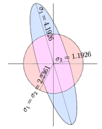
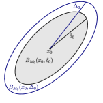
Figure 3: (Left) Illustration of optimality condition of Thm. 2 for $F=\begin{bmatrix}1&1\\ -4&1\end{bmatrix}$, $F$ has conjugate pair of complex eigenvalues $1\pm i\sqrt{2}$. SVD decomposition of $F$ reveals it rotates and transforms unit disc into blue ellipse, where the radii are equal to the singular values ($\sigma_{1}=4.1926$, $\sigma_{2}=1.1926$), resp. SVD of $\hat{A}_{1}F\hat{A}^{-1}_{1}$ reveals, however, that two singular values are equal $\sigma_{1}=\sigma_{2}=2.2361$. Recall SF is equal to $\sigma_{1}$; although the two “balls” have the same volume, the circular one results in a significantly smaller SF ($2.2361$ versus $4.1926$). (Right) The larger ball $B_{M_{0}}(x_{0},\Delta_{0})$ depicted in blue, is a conservative over-estimate for the reachtube continuous segment $\text{Reach}\left([t_{0},t_{0}+h],\mathcal{X}\right)$, that is, it is such that $\chi_{t_{0}}^{[t_{0},t_{0}+h]}\left(B_{M_{0}}(x_{0},\delta_{0})\right)\subset B_{M_{0}}\left(x_{0},\Delta_{0}\right)$.

IV Conservative Continuous-Time Reachtubes

We present a simple ellipsoidal construction for tightly over-estimating the continuous-time segments of a reachtube. For a given ellipsoidal bound for the set of initial states of radius $\delta_{0}$, if the radius of this bound is bloated as in Figure 3 (Right), up to a computable bound $\Delta_{0}$, such that:

$$\delta_{0}+\max_{\begin{subarray}{c}x\in B_{M_{0}}(x_{0},\Delta_{0})\\ s\in[0,h]\end{subarray}}{\left\|h\cdot f(t_{0}\,{+}\,s,x)\right\|_{M_{0}}}\leq\Delta_{0},$$

where $h$ is a time increment and $f$ is the dynamics of the Cauchy problem (1), then the resulting ellipsoid becomes a tight overestimate of the whole continuous segment $\chi_{t_{0}}^{[t_{0},t_{0}+h]}(x)\subset\mathbb{R}^{n}$, representing the set of all values $\chi_{t_{0}}^{t}(x)$ of the solution flow of  (1), for all times $t\,{\in}\,[t_{0},t_{0}+h]$.

Lemma 1

Given the Cauchy problem (1) with $x_{0}\in\mathbb{R}^{n}$ the initial state, $t_{0}$ the current time, $h$ the current time-step, and $\chi_{t_{0}}^{t}(x)$ the solution flow, let $\Delta\,{>}\,0$ and $M\succ 0$ be a matrix defining the metric space being used. Then:

$$\max_{\begin{subarray}{c}x\in B_{M}(x_{0},\Delta)\\ s\in[0,h]\end{subarray}}{\left\|h\cdot f(t_{0}\,{+}\,s,x)\right\|_{M}}\leq\Delta\\[-5.69054pt] \Rightarrow\chi_{t_{0}}^{[t_{0},t_{0}+h]}(x_{0})\subseteq B_{M}(x_{0},\Delta)$$

Proof:

Let $\mathcal{C}([t_{0},t_{0}+h],\mathbb{R}^{n})$ denote the space of continuous and differentiable functions defined over the interval $[t_{0},t_{0}+h]$ and domain $\mathbb{R}^{n}$. Define the operator $T_{x_{0}}\colon\mathcal{C}([t_{0},t_{0}+h],\mathbb{R}^{n})\to\mathcal{C}([t_{0},t_{0}+h],\mathbb{R}^{n})$ as follows:

$$\begin{array}[]{c}T_{x_{0}}(\chi)(h^{\prime})=x_{0}+\int_{0}^{h^{\prime}}{f(t_{0}\,{+}\,s,\chi_{t_{0}}^{t_{0}\,{+}\,s}(x_{0}))}\,ds,\ h^{\prime}\in[0,h].\end{array}$$

Let $\mathcal{C}([t_{0},t_{0}+h],B_{M}(x_{0},\Delta))\,{\subset}\,\mathcal{C}([t_{0},t_{0}\,{+}\,h],\mathbb{R}^{n})$ be the subspace of continuous, differentiable, and bounded functions having their range contained within $B_{M}(x_{0},\Delta)$. We show that $T_{x_{0}}$ maps $\mathcal{C}([t_{0},t_{0}+h],B_{M}(x_{0},\Delta))$ into itself. Let $\chi\in\mathcal{C}([t_{0},t_{0}+h],B_{M}(x_{0},\Delta))$. Then $\|T_{x_{0}}(\chi)(h^{\prime})-x_{0}\|_{M}$ is bounded as follows:

$$\left\|\int_{0}^{h^{\prime}}{f(t_{0}\,{+}\,s,\chi_{t_{0}}^{t_{0}\,{+}\,s}(x_{0}))}\,ds\right\|_{M}\leq\\[-5.69054pt] \int_{0}^{h^{\prime}}{\left\|f(t_{0}\,{+}\,s,\chi_{t_{0}}^{t_{0}\,{+}\,s}(x_{0}))\right\|_{M}}\,ds\leq\\[-5.69054pt] \max_{\begin{subarray}{c}x\in B_{M}(x_{0},\Delta)\\ s\in[0,h^{\prime}]\end{subarray}}{\left\|h^{\prime}\cdot f(t_{0}\,{+}\,s,x)\right\|_{M}}\leq\\[-5.69054pt] \max_{\begin{subarray}{c}x\in B_{M}(x_{0},\Delta)\\ s\in[0,h]\end{subarray}}{\left\|h\cdot f(t_{0}\,{+}\,s,x)\right\|_{M}}.$$

The inequalities are due to the fact that $\chi\in\mathcal{C}([t_{0},t_{0}+h],B_{M}(x_{0},\Delta))$. The second and the third ones allow us to compute the integral explicitly. Now using the assumption $\max_{\begin{subarray}{c}x\in B_{M}(x_{0},\Delta)\\ s\in[0,h]\end{subarray}}{\left\|h\cdot f(t_{0}\,{+}\,s,x)\right\|_{M}}\leq\Delta$, we can infer that:

$$T_{x_{0}}(\chi)(h^{\prime})\in B_{M}(x_{0},\Delta)\text{ for all }h^{\prime}\in[0,h].$$

As $\chi$ was arbitrary, $T_{x_{0}}\left(\mathcal{C}([t_{0},t_{0}+h],B_{M}(x_{0},\Delta))\right)$ is a subset of the class of continuous functions $\mathcal{C}([t_{0},t_{0}+h],B_{M}(x_{0},\Delta))$. For instance, the standard Schauder’s fixed-point theorem argument shows that the solution of (1) with the initial condition $(t_{0},x_{0})$ – a fixed point of $T$, satisfies $\chi_{t_{0}}^{t_{0}+h^{\prime}}(x_{0})\in B_{M}(x_{0},\Delta),\forall{h^{\prime}}\in[0,h].$ ∎

Theorem 3 (Optimization for a tight overestimate)

Consider the Cauchy problem (1), and let $\chi_{t_{0}}^{t}(x)$ denote the flow generated by (1). Let $x_{0}\in\mathbb{R}^{n}$ be an initial state, $t_{0}$ be the current time, $h$ be the current time-step, and $M_{0}\succ 0$ be a matrix defining a metric. Let $B_{M_{0}}(x_{0},\delta_{0})$ be given (output from the LRT algorithm). Then for all $\bar{x}\in B_{M_{0}}(x_{0},\delta_{0})$:

$$\delta_{0}+\max_{\begin{subarray}{c}x\in B_{M_{0}}(x_{0},\Delta_{0})\\ s\in[0,h]\end{subarray}}{\left\|h\cdot f(t_{0}+s,x)\right\|_{M_{0}}}\leq\Delta_{0}\Rightarrow\\[-5.69054pt] \chi_{t_{0}}^{[t_{0},t_{0}+h]}(\bar{x})\subset B_{M_{0}}(x_{0},\Delta_{0})$$ (15)

Proof:

Pick any $\bar{x}\in B_{M_{0}}(x_{0},\delta_{0})$. Rewriting the current assumption as

$$\max_{\begin{subarray}{c}x\in B_{M_{0}}(\bar{x},\Delta_{0}-\delta_{0})\\ s\in[0,h]\end{subarray}}{\left\|h\cdot f(t_{0}+s,x)\right\|_{M_{0}}}\leq\\ \max_{\begin{subarray}{c}x\in B_{M_{0}}(x_{0},\Delta_{0})\\ s\in[0,h]\end{subarray}}{\left\|h\cdot f(t_{0}+s,x)\right\|_{M_{0}}}\leq\Delta_{0}-\delta_{0},$$

the first inequality holds from $B_{M_{0}}(\bar{x},\Delta_{0}-\delta_{0})\subset B_{M_{0}}(x_{0},\Delta_{0})$. From Lemma 1 it immediately follows that

$$\chi_{t_{0}}^{[t_{0},t_{0}+h]}(\bar{x})\subset B_{M_{0}}(\bar{x},\Delta_{0}-\delta_{0})\subset B_{M_{0}}(x_{0},\Delta_{0}).$$

∎

The following Corollary is obtained by performing minor changes to the proof of Theorem 3.

Corollary 1 (Applying Thm. 3 backwards in time)

Given the ODE system (1), with $x_{0}\in\mathbb{R}^{n}$ the initial state, $t_{0}$ the current time, $h$ the current time-step, and $\chi_{t_{0}}^{t}(x)$ the solution flow, let $\Delta_{0}\,{>}\,0$ and $M_{0}\succ 0$ define the metric space used. Then for all $\bar{x}\in B_{M_{0}}(x_{0},\delta_{0})$:

$$\delta_{0}+\max_{\begin{subarray}{c}x\in B_{M_{0}}(x_{0},\Delta_{0})\\ s\in[0,h]\end{subarray}}{\left\|h\cdot f(t_{0}\,{-}\,s,x)\right\|_{M_{0}}}\leq\Delta_{0}\Rightarrow\\[-5.69054pt] \chi_{t_{0}}^{[t_{0}-h,t_{0}]}(\bar{x})\subseteq B_{M_{0}}(x_{0},\Delta_{0}).$$ (16)

Remark 2

An important consequence of Theorem 3 and Corollary 1 is that for time invariant systems, conditions (15),(16) imply

$$\delta_{0}+\max_{x\in B_{M_{0}}(x_{0},\Delta_{0})}{\left\|h\cdot f(x)\right\|_{M_{0}}}\leq\Delta_{0}\Rightarrow\\ \chi_{t_{0}}^{[t_{0}-h,t_{0}]}(\bar{x})\text{ and }\chi_{t_{0}}^{[t_{0},t_{0}+h]}(\bar{x})\subset B_{M_{0}}(x_{0},\Delta_{0}).$$ (17)

Hence, ball $B_{M_{0}}(x_{0},\Delta_{0})$ covers both the forward and backward orbits locally for all times $[t_{0}-h,t_{0}+h]$ that initiate within $B_{M_{0}}(x_{0},\delta_{0})$.

V Nonconvex Optimization in CLRT

V-A Bounding the Maximal Vector Field in Metric $\mathbf{M}_{0}$

In Theorem 3 of Section VI, we give a computable condition for determining a tight overestimate of a continuous reachtube segment, based on the set of initial states in a ball $B_{M_{0}}(x_{0},\delta_{0})$, in some metric $M_{0}\succ 0$. More precisely, a conservative radius (denoted by $\Delta_{0}$) of the continuous reachtube segment overestimate needs to satisfy:

$$\max_{\begin{subarray}{c}x\in B_{M_{0}}(x_{0},\Delta_{0})\\ s\in[0,h]\end{subarray}}{\left\|h\cdot f(t_{0}+s,x)\right\|_{M_{0}}}\leq\Delta_{0}-\delta_{0}.$$ (18)

Verifying conservativeness of $\Delta_{0}$ requires bounding the maximal vector field value in a metric given by $M_{0}$, as in the left-hand side of (18). We emphasize that any convex optimization program (COP) for verifying this condition will not be sound, as we neither assume convexity of $f$ in (1), nor does it follow from our approach.

An interesting problem in this case is to see if $f$ restricted to times from time-step adaptation scheme based on IST is locally convex. If $f$ is still nonconvex, one may need to further decrease the time-step such that $f$ becomes convex in this small range, and a COP can be used to find $\Delta_{0}$ satisfying (18).

Due to a possible lack of convexity, we restate the global optimization problem of bounding the left-hand side of (18) as one of $\varepsilon$-satisfiability over the reals [13, 14]. (Normally referred to as $\delta$-satisfiability, we use the name $\varepsilon$-satisfiability to avoid confusion with $\delta_{0}$, denoting a ball radius in our context.) For an initial guess for $\Delta_{0}\,{-}\,\delta_{0}$, given for example by COP, we define the following quantified formula:

$$\exists_{x\in B_{M_{0}}(x_{0},\Delta_{0})}\exists_{s\in[0,h]}{\|h\,{\cdot}\,f(t_{0}+s,x)\|_{M_{0}}>\Delta_{0}\,{-}\,\delta_{0}}.$$ (19)

We provide below an interpretation of the $\varepsilon$-satisfiability answers for (19), where the first answer tells us that $\Delta_{0}\,{-}\,\delta_{0}$ is a good bound: UNSAT means that $\forall x\,{\in}\,B_{M_{0}}(x_{0},\Delta_{0})$, $\forall s\,{\in}\,[0,h]$, the inequality $\|h\,{\cdot}\,f(t_{0}+s,x)\|_{M_{0}}\leq\Delta_{0}-\delta_{0}$ holds, and hence (18) is satisfied. $\varepsilon$-SAT means that an $\varepsilon$-weakening is satisfiable, i.e., $\exists x$ $\in$ $B_{M_{0}}(x_{0},\Delta_{0})$, $\exists s$ $\in$ $[0,h]$, $\left|\|h\,{\cdot}\,f(t_{0}+s,x)\|_{M_{0}}\,{-}\,\varepsilon\right|>\Delta_{0}\,{-}\,\delta_{0}$.

VI The CLRT Reachability Algorithm

Notation. By $[x]$ we denote a product of intervals (a box), i.e., a compact and connected set $[x]\subset\mathbb{R}^{n}$. We will use the same notation for interval matrices.

Definition 2

Given an initial set $\mathcal{X}$, initial time $t_{0}$, and target time $t_{1}\geq t_{0}$, we call the following compact sets:

• $\mathcal{W}\,{\subset}\,\mathbb{R}^{n}$ a tight reach-set enclosure if $\forall{x}\,{\in}\,\mathcal{X}.~{}\chi_{t_{0}}^{t_{1}}(x)\in\mathcal{W}$.

• $\mathcal{F}\,{\subset}\,\mathbb{R}^{n\times n}$ a conservative gradient enclosure if $\forall{x}\,{\in}\,\mathcal{X}.~{}\nabla_{x}\chi_{t_{0}}^{t_{1}}(x)\in\mathcal{F}$.

Given a set $\mathcal{X}\,{\subset}\,\mathbb{R}^{n}$ and a time $t_{0}$, we call a state $x\,{\in}\,\mathbb{R}^{n}$ reachable within time interval $[t_{1},t_{2}]$ if there is an initial state $x_{0}\,{\in}\,\mathcal{X}$ at time $t_{0}$ and a time $t\in[t_{1},t_{2}]$, such that $x=\chi_{t_{0}}^{t}(x_{0})$. The set of all reachable states in interval $[t_{1},t_{2}]$ is called the reach set and is denoted by $\mbox{Reach}((t_{0},\mathcal{X}),[t_{1},t_{2}])$.

Definition 3 ([11] Def. 2.4)

Given an initial set $\mathcal{X}$, initial time $t_{0}$, and time bound $T$, a $((t_{0},X),T)$-reachtube of (1) is a sequence of time-stamped sets $(R_{1},t_{1}),\dots,(R_{k},t_{k})$ satisfying the following properties: (1) $t_{0}\leq t_{1}\leq\dots\leq t_{k}=T$, (2) $\mbox{Reach}((t_{0},\mathcal{X}),[t_{i-1},t_{i}])\subset R_{i},\forall i=1,\dots,k$.

We shall henceforth simply use the name reachtube overestimate of the flow defined by ODE system (1). We now present the CLRT algorithm for computing tight over-estimations for segments $(R_{i},t_{i})$, with $\mbox{Reach}((t_{0},\mathcal{X}),[t_{i-1},t_{i}])\,{\subset}\,R_{i}$, whose union makes up the complete $((t_{0},X),T)$-reachtube of (1). CLRT therefore computes the whole reachtube overestimate of the flow defined by (1). LRT computes discrete-time slices of the CLRT reachtube.

Input:ODE system (1); Parameters:Time horizon $T$, initial time $t_{0}$, number of discrete-time steps $k$, and initial time increment $h\,{=}\,T{/}k$ (observe that $h$ may change during execution of the algorithm due to the IST condition); Metric: Positive-definite symmetric matrix $M_{0}\succ 0$ for initial norm. Initial region: Bounds $[x_{0}]\,{\subset}\,\mathbb{R}^{n}$ for the center, and the radius $\delta_{0}\,{>}\,0$, for the ball $B_{M_{0}}(x_{0},\delta_{0})$ with norm $M_{0}$ at initial time $t_{0}$. IST threshold: $\varepsilon_{IST}>0$ – threshold used to check for smallness of the IST displacement gradient tensor. Increment for $\varepsilon$-satisfiability: $C_{\delta}>1$ – increment used for iterative validation of upper bound for maximal speed within bounds using $\varepsilon$-satisfiability. Norm switch threshold $C_{M}>0$ – threshold value used to decide if the metric space used should be updated to a new $\hat{M}_{1}$.

Output: $\{[x_{j}]\}_{j=1}^{k}\,{\subset}\,\mathbb{R}^{n\times{k}}$: Interval enclosures for ball centers $x_{j}$ at time $t_{0}\,{+}\,jh$. $\{M_{j}\}_{j=1}^{k}$: Norms defining metric spaces for the ball enclosures. $\{\Delta_{j}\}_{j=1}^{k}\,{\in}\,\mathbb{R}_{+}^{k}$: Radii of the ball enclosures at $x_{j}$, for $j=1,\dots,k$.
Begin CLRT

1. Begin IST

   1. Compute overestimates for the (deformation) gradient tensor $[\nabla_{x}\chi_{t_{0}}^{t_{1}}\left([B([x_{0}],\delta_{0}\right)])]$, and for the displacement gradient tensor $[\nabla_{X}{u(X,t)}]$.

   2. Adjust the time increment $h$ by halving it until $\|[\nabla_{X}{u(X,t)}]\|<\varepsilon_{IST}\text{ is satisfied.}$

   3. Set $t_{1}\,{=}\,t_{0}\,{+}\,h$.

2. End IST, Begin improved LRT (see section III)

   1. Compute an enclosure for $[x_{1}]$, i.e. the center of the reachtube at $t_{1}$, and for the gradient of the flow initiating at $[x_{0}]$, i.e. $[D_{x}\chi_{t_{0}}^{t_{1}}([x_{0}])]$.

   2. Compute the optimal deformation metric $\hat{M}_{1}(F)=\hat{A}_{1}(F)^{T}\hat{A}_{1}(F)$ (see Def. 1) for $F=\operatorname{mid}{[D_{x}\chi_{t_{0}}^{t_{1}}([x_{0}])]}$.

   3. If it holds that $M_{0}\text{-SF}>C_{M}\cdot\hat{M}_{1}\text{-SF}$, set $M_{1}=\hat{M}_{1}$. Otherwise, set $M_{1}=M_{0}$.

   4. Compute an upper bound for $M_{0,1}$-SF (12) (denoted $\Lambda$), and compute the discrete-time reachtube overestimate at time $t_{1}$:

      $$B_{1}=B_{M_{1}}([x_{1}],\Lambda\cdot\delta_{0}),\quad\mbox{Reach}((t_{0},\mathcal{X}),t_{1})\subset B_{1}.$$

3. End improved LRT, Begin continuous part

   1. Initialize $\Delta_{0}=\delta_{0}\cdot C_{\delta}$.

   2. Solve a nonlinear convex optimization problem to compute $\tilde{\delta}$, an approximate maximum of the left-hand side of (18), and set $\hat{\Delta}_{0}=\delta_{0}+\tilde{\delta}$.

   3. Update $\tilde{\delta}$ to satisfy an upper bound for the global maximum of the left-hand side of (18) as follows:

      1. check following SMT formula using dReal:

         $$\begin{split}\exists_{x\in B_{M_{0}}(x_{0},\hat{\Delta}_{0})}\exists_{s\in[0,h]}\|h\,{\cdot}\,f(t_{0}\,{+}\,s,x)\|_{M_{0}}\\ >\hat{\Delta}_{0}\,{-}\,\delta_{0}=\tilde{\delta}.\end{split}$$

      2. If dReal returns UNSAT, then $\tilde{\delta}$ is an upper bound for the global maximum. Otherwise, set $\tilde{\delta}=\tilde{\delta}\cdot C_{\delta}$, and $\hat{\Delta}_{0}=\delta_{0}+\tilde{\delta}$, go to step i.

   4. If we set $\Delta_{0}=\hat{\Delta}_{0}$, then (18) holds, and thus $\Delta_{0}$ is an appropriate radius for the continuous tube. Otherwise, we set $\Delta_{0}=\Delta_{0}\cdot C_{\delta}$ and go to step (b).

4. End continuous part

5. For next interval, reset the initial time to $t_{1}$, and consider the enclosure for the new initial set as $B_{M_{1}}([x_{1}],\delta_{1})$.

6. Save $B_{M_{0}}([x_{0}],\Delta_{0})$ satisfying

   $$\mbox{Reach}((t_{0},B_{M_{0}}([x_{0}],\delta_{0})),[t_{0},t_{1}])\subset B_{M_{0}}([x_{0}],\Delta_{0}).$$

7. If $t_{1}\geq T$ terminate. Otherwise, go back to 1.

End CLRT

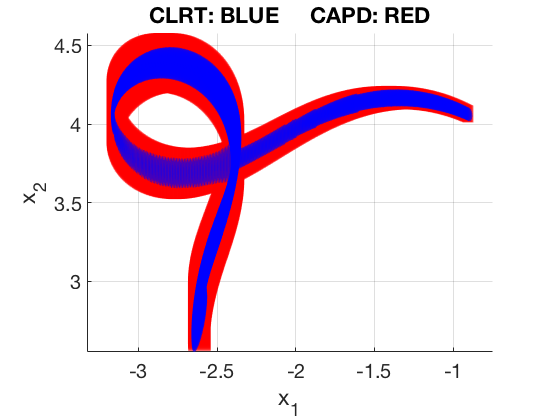
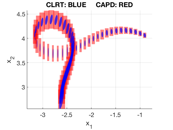
Figure 4: Comparison of continuous-time reachtubes for Dubins car example with nonlinear steering function $\dot{x}=\cos{\theta},\dot{y}=\sin{\theta},\dot{\theta}=x\sin{t}$. See also Table I, row D3. Projection of computed bounds onto $x,y$ is shown. The left figure presents all tube segments for times within $[5,10]$, whereas the right figure shows one segment per $20$ sequential segments computed by the algorithms. Set of initial states has center at $(0,0,0.7854)$ and radius $0.01$.

Proposition 1

Assume that the rigorous tool used by LRT produces conservative gradient enclosures for (1), and that LRT terminates on the provided inputs. Let $[t_{0},T]$ be the whole time interval, which is traversed by CLRT in $k$ steps. Then, the output of the CLRT is a tight reachtube over-approximation of (1) for all times in $[t_{0},T]$; i.e., for $t_{k+1}=T$: $\mbox{Reach}((t_{0},\mathcal{X}),[t_{j},t_{j+1}])\subset B_{M_{j}}([x_{j}],\Delta_{j})\text{, for }j=1,\dots,k$

Proof:

The proof follows from [8, Theorem LRT-Conservativity], Theorems 2 and 3, and the soundness of the $\varepsilon$-satisfiability algorithm. ∎

CLRT is also an efficient algorithm. This follows from the use of IST to derive the proper time increments $h$, and the use of nonlinear COP to finding initial estimates $\hat{\Delta}_{0}$, which are passed to the $\varepsilon$-satisfiability algorithm.

VII Implementation and Experimental Results

We implemented a prototype of CLRT in C++. Our implementation is based on interval arithmetic; i.e., all variables used in the algorithm are over intervals, and all computations performed are executed using interval arithmetic. The prototype runs the CLRT algorithm in two passes. In the first pass, overestimates for discrete segments of reachtube are generated using the LRT algorithm. In the second pass, we run the procedure for constructing continuous tight overestimates, in each time interval from the discrete ones. In the first pass, we also compute optimal norms by using the analytical formulas from Def. 1.

To compute an upper bound $\Lambda$ for the square-root of the maximal eigenvalue of all symmetric matrices in some interval bounds, we implemented in C++ several algorithms [15, 25, 24] and used the tightest result available. Source code, numerical data, and readme file describing compilation procedure for LRT are available online [16].

Table I summarizes CLRT’s performance on a set of benchmarks (see [8] for details). Fig. 4 presents a visual comparison of computed bounds for benchmark D(3). The table illustrates that CLRT performs much better in all cases except Mitchell Schaeffer model and biology model. Typically our algorithm works better for stable systems, whereas CAPD is specialized for chaotic system or a system containing unstable regime in its dynamics.

VIII Related Work

Computing the exact reachable set of (1) is hard, as these systems do not admit a closed-form solution. Instead, a conservative (over-approximating) reachtube is computed to determine if an unsafe region can possibly be reached. Existing tools and techniques for conservative reachtube computation can be classified into three categories according to the time-space approximation they perform : (1) Taylor-expansion in time, variational-expansion in space (wrapping-effect reduction) of the solution set, e.g., CAPD [5, 27], VNode-LP [22, 21], CORA [2]. (2) Taylor-expansion in time and space of the solution set, e.g., Cosy Infinity [18, 4, 19], Flow* [6, 7]. (3) Bloating-factor-based and discrepancy-function-based [11, 12]. Other approaches to compute conservative reachtubes include the Hamilton-Jacobi-based method [20, 3] and the recently developed Runge-Kutta-based method [1]. In this paper, we present an alternative (and orthogonal) technique based on a stretching factor that is derived from an over-approximation of the gradient of the solution-flows (also known as the sensitivity matrix) and the deformation tensor.

IX Conclusions and Future Work

We presented CLRT, a new algorithm for computing tight reachtubes for solution flows of nonlinear systems. CLRT synergistically combines a number of techniques, e.g. finite and infinitesimal strain theory, computation of tightest deformation metric using explicit analytical formulas, $\delta$-satisfiability, and nonconvex optimization.

Future work includes distributing a C++ implementation of CLRT, and extending our approach to Hybrid dynamical systems and PDEs. The implementation of our tool will significantly improve its performance on large-scale nonlinear and continuous dynamical systems.

Table I: Performance comparison CAPD. We use following labels: B(2)- Brusselator, I(2)- Inverse Van der Pol oscillator, D(3)- Dubins Car, F(2)- Forced Van der Pol oscillator, M(2)- Mitchell Schaeffer cardiac-cell model, R(4)- Robot arm, O(7)- Biology model, P(12)-Polynomial system (number in parenthese denotes dimension). T: time horizon, dt: time step, ID: initial diameter in each dimension, TV: total volume of reachtubes in T, AV: average volume of reachtubes in T.

BM	$T$	ID	CLRT		CAPD
			TV	AV	TV	AV
B(2)	$10$	$0.02$	$\mathbf{0.21}$	$\mathbf{2\times 10^{-4}}$	$0.59$	$6\times^{-4}$
I(2)	$10$	$0.02$	$\mathbf{0.13}$	$\mathbf{6\times 10^{-5}}$	$0.15$	$7\times 10^{-5}$
D(3)	$10$	$0.02$	$\mathbf{0.24}$	$\mathbf{1\times 10^{-4}}$	$2.8$	$1\times 10^{-3}$
M(2)	$10$	$0.002$	$0.005$	$2\times 10^{-5}$	$\mathbf{0.003}$	$\mathbf{2\times 10^{-6}}$
R(4)	$10$	$0.02$	$\mathbf{1.2}$	$\mathbf{1\times 10^{-12}}$	$6.2$	$1\times 10^{-10}$
O(7)	$5$	$10^{-4}$	$7\times 10^{-16}$	$7\times 10^{-19}$	$\mathbf{6\times 10^{-20}}$	$\mathbf{6\times 10^{-23}}$
P(12)	$0.5$	$10^{-4}$	$\mathbf{10^{-34}}$	$\mathbf{10^{-36}}$	$6\times 10^{26}$	$6\times 10^{-26}$

IX-A Acknowledgements

We thank the anonymous reviewers for their valuable comments. Research supported by: U.S. Air Force (AFRL) Contract No. FA9550-15-C-0030; NSF CPS-1446832; NSF IIS-1447549; NSF CNS-1445770; DARPA Assured Autonomy Program.

References

- [1] J. Alexandre dit Sandretto and A. Chapoutot. Validated explicit and implicit Runge-Kutta methods. Reliable Computing electronic edition, 22, July 2016.
- [2] M. Althoff. An introduction to CORA 2015. In Proc. of the Workshop on Applied Verification for Continuous and Hybrid Systems, 2015.
- [3] S. Bansal, M. Chen, S. Herbert, and C. J. Tomlin. Hamilton-Jacobi reachability: a brief overview and recent advances. In Decision and Control (CDC), 2017 IEEE 56th Annual Conference on, pages 2242–2253. IEEE, 2017.
- [4] M. Berz and K. Makino. Verified integration of odes and flows using differential algebraic methods on high-order taylor models. Reliable Computing, 4(4):361–369, 1998.
- [5] M. Capiński, J. Cyranka, Z. Galias, T. Kapela, M. Mrozek, P. Pilarczyk, D. Wilczak, P. Zgliczyński, and M. Żelawski. CAPD - computer assisted proofs in dynamics, a package for rigorous numerics, http://capd.ii.edu.pl/. Technical report, Jagiellonian University, Kraków, 2016.
- [6] X. Chen, E. Abraham, and S. Sankaranarayanan. Taylor model flowpipe construction for non-linear hybrid systems. In Proceedings of the 2012 IEEE 33rd Real-Time Systems Symposium, RTSS ’12, pages 183–192, Washington, DC, USA, 2012. IEEE Computer Society.
- [7] X. Chen, E. Ábrahám, and S. Sankaranarayanan. Flow*: an analyzer for non-linear hybrid systems, pages 258–263. Springer Berlin Heidelberg, Berlin, Heidelberg, 2013.
- [8] J. Cyranka, M. A. Islam, G. Byrne, P. Jones, S. A. Smolka, and R. Grosu. Lagrangian reachabililty, pages 379–400. Springer International Publishing, Cham, 2017.
- [9] A. Donzé. Breach, a toolbox for verification and parameter synthesis of hybrid systems, pages 167–170. Springer Berlin Heidelberg, Berlin, Heidelberg, 2010.
- [10] A. Donzé and O. Maler. Systematic simulation using sensitivity analysis, pages 174–189. Springer Berlin Heidelberg, Berlin, Heidelberg, 2007.
- [11] C. Fan, J. Kapinski, X. Jin, and S. Mitra. Locally optimal reach set over-approximation for nonlinear systems. In Proceedings of the 13th International Conference on Embedded Software, EMSOFT ’16, pages 6:1–6:10, New York, NY, USA, 2016. ACM.
- [12] C. Fan and S. Mitra. Bounded verification with on-the-fly discrepancy computation, pages 446–463. Springer International Publishing, Cham, 2015.
- [13] S. Gao, J. Avigad, and E. M. Clarke. -complete decision procedures for satisfiability over the reals. In B. Gramlich, D. Miller, and U. Sattler, editors, Automated Reasoning, pages 286–300, Berlin, Heidelberg, 2012. Springer Berlin Heidelberg.
- [14] S. Gao, S. Kong, and E. M. Clarke. dreal: An smt solver for nonlinear theories over the reals. In M. P. Bonacina, editor, Automated Deduction – CADE-24, pages 208–214, Berlin, Heidelberg, 2013. Springer Berlin Heidelberg.
- [15] M. Hladík, D. Daney, and E. Tsigaridas. Bounds on real eigenvalues and singular values of interval matrices. SIAM Journal on Matrix Analysis and Applications, 31(4):2116–2129, 2010.
- [16] M. A. Islam and J. Cyranka. CLRT implementation. https://github.com/mdaislam006/CLRT.git, 2018.
- [17] J. Maidens and M. Arcak. Reachability analysis of nonlinear systems using matrix measures. IEEE Transactions on Automatic Control, 60(1):265–270, Jan 2015.
- [18] K. Makino and M. Berz. Cosy infinity version 9. Nuclear Instruments and Methods in Physics Research Section A: Accelerators, Spectrometers, Detectors and Associated Equipment, 558(1):346–350, 2006.
- [19] K. Makino and M. Berz. Rigorous integration of flows and odes using taylor models. Symbolic Numeric Computation, pages 79–84, 2009.
- [20] I. M. Mitchell and C. J. Tomlin. Overapproximating reachable sets by Hamilton-Jacobi projections. journal of Scientific Computing, 19(1-3):323–346, 2003.
- [21] N. S. Nedialkov. Interval tools for odes and daes. In 12th GAMM - IMACS International Symposium on Scientific Computing, Computer Arithmetic and Validated Numerics (SCAN 2006), pages 4–4, Sept 2006.
- [22] N. S. Nedialkov. VNODE-LP—a validated solver for initial value problems in ordinary differential equations. In Technical Report CAS-06-06-NN. 2006.
- [23] R. T. Pierrehumbert. Large‐scale horizontal mixing in planetary atmospheres. Physics of Fluids A: Fluid Dynamics, 3(5):1250–1260, 1991.
- [24] J. Rohn. Bounds on eigenvalues of interval matrices. ZAMMZ.Angew.Math.Mech., 78:1049–1050, 1998.
- [25] S. M. Rump. Computational error bounds for multiple or nearly multiple eigenvalues. Linear Algebra and its Applications, 324(1):209 – 226, 2001. Linear Algebra in Self-Validating Methods.
- [26] W. S. Slaughter. The linearized theory of elasticity. Springer Science+Business Media, LLC, 2012.
- [27] D. Wilczak and P. Zgliczyński. -Lohner algorithm. Schedae Informaticae, 2011(Volume 20), 2012.