From Kondo effect to weak-link regime in quantum spin-1/2 spin chains

Abstract

We analyze the crossover from Kondo to weak-link regime by means of a model of tunable bond impurities in the middle of a spin-1/2 XXZ Heisenberg chain. We study the Kondo screening cloud and estimate the Kondo length by combining perturbative renormalization group approach with the exact numerical calculation of the integrated real-space spin-spin correlation functions. We show that, when the spin impurity is symmetrically coupled to the two parts of the chain with realistic values of the Kondo coupling strengths and spin-parity symmetry is preserved, the Kondo length takes values within the reach of nowadays experimental technology in ultracold-atom setups. In the case of non-symmetric Kondo couplings and/or spin parity broken by a nonzero magnetic field applied to the impurity, we discuss how Kondo screening redistributes among the chain as a function of the asymmetry in the couplings and map out the shrinking of the Kondo length when the magnetic field induces a crossover from Kondo impurity to weak-link physics.

I Introduction

The Kondo effect has been first seen in conducting metals containing magnetic impurities, such as Co atoms; it consists in an impurity-triggered, low-temperature increase in the metal resistanceKondo (1964); Hewson (1993); Kouwenhoven and Glazman (2001). Physically, Kondo effect is the result of nonperturbative spin-flip processes involving the spin of a magnetic impurity and of the itinerant conduction electrons in the metal, which results in the formation, for vanishing temperature, of a strongly correlated Kondo state between the impurity and the conduction electrons Kondo (1964); Hewson (1993). In the Kondo state, spins cooperate to dynamically screen the magnetic moment of the impurity Kondo (1964); Hewson (1993); Nozières (1974). The specific properties of the correlated state depend on, e.g., the number of independent “spinful channels” of conduction electrons participating to the screening versus the total spin of the magnetic impurity. Denoting the latter by $s$, when the number of independent screening channels $k$ is equal to $2s$, in the Kondo state the impurity spin is perfectly screened, which makes the screened impurity act as a localized scatterer with well-defined single-particle phase shift at the Fermi level. This corresponds to the onset of Nozières Fermi-liquid state Nozières (1974, 1978); at variance, when $k>2s$, the Kondo state is characterized by impurity “overscreening”, which determines its peculiar, non Fermi-liquid properties Affleck and Ludwig (1993, 1991).

Over the last decades, the Kondo effect emerged as a paradigm in the study of strongly correlated electronic states, providing an arena where to test many-body techniques, both analytical and numerical Bulla et al. (2008). Also, the realization of a Kondo interaction involving Majorana fermion modes arising at the endpoints of one-dimensional (1D) topological superconductors has paved the way to a novel, peculiar form of “topological” Kondo effect, sharing many common features with the overscreened multichannel Kondo effect Béri and Cooper (2012); Altland et al. (2014); Buccheri et al. (2015); Eriksson et al. (2014). Besides its fundamental physics aspects, the Kondo effect has attracted a renewed theoretical as well as experimental interest, since it has been possible to realize it with controlled parameters in quantum dots with either metallic Alivisatos (1996); Kouwenhoven and Marcus (1998); Goldhaber-Gordon et al. (1998); Cronenwett et al. (1998), or superconducting leads Avishai et al. (2001); Choi et al. (2004); Campagnano et al. (2004). This led to the possibility of using the Kondo effect to design quantum circuits with peculiar conduction properties, such as a conductance reaching the maximum value allowed by quantum mechanics for a single conduction channel Kouwenhoven and Glazman (2001).

Formally, the Kondo effect is determined by a renormalization group (RG) crossover between quantum impurity ultraviolet and infrared fixed points (corresponding to the Kondo state). Typically, for a spin-1/2 impurity, near the ultraviolet fixed point (high energy), the coupling between the quantum impurity and the spin of conduction electrons is weak, thus merely providing a perturbative correction to the decoupled dynamics of the two of them. At variance, near the infrared fixed point (low energy), the conduction electrons in the Fermi sea adjust themselves to screen the impurity spin into a localized spin singlet. Regarding the relevant energy window for the process, the impurity spin screening requires a cooperative effect of electrons with energies all the way down to $k_{B}T_{K}$, with $k_{B}$ being the Boltzmann constant (which we set to $1$ henceforth) and $T_{K}$ the Kondo temperature, that is, a temperature scale invariant under RG trajectories and dynamically generated by the Kondo dynamics Hewson (1993). At energies $\sim T_{K}$ a crossover takes place, between the perturbative dynamics of the impurity spin weakly coupled to itinerant electrons and the nonperturbative onset of the Kondo state. The possibility of using the Fermi velocity $v_{f}$ to trade an energy scale $E_{*}$ for a length scale $L_{*}\sim v_{f}/E_{*}$ led to the proposal that the crossover might be observed in real space, as well Wilson (1975); Nozières (1974). Switching from an energy to a length reference scale implies that dynamical impurity spin screening has now to be thought of as a real-space phenomenon, with the net effect of substituting, as a reference scale for screening, the temperature with the distance from the impurity $x$. In other words, a physical quantity depending on the distance $x$ from the impurity is expected (on moving away from the impurity) to exhibit a crossover from a perturbative behavior controlled by the ultraviolet fixed point at small $x$ to a nonperturbative behavior controlled by the Kondo state at large $x$, the crossover taking place at a scale $\xi_{K}\sim v_{f}/T_{K}$. Such value $\xi_{K}$ can accordingly be regarded as the size of the electronic cloud screening the impurity spin: for this reason, it is typically referred to as the Kondo screening length.

The presence of a Kondo cloud (KC) is well-grounded on the theory side and it has also been recently proposed that an analogous phenomenon takes place at a Majorana mode coupled to a 1D quantum wire Affleck and Giuliano (2014). However, any attempt to experimentally detect it at magnetic impurities in metals has so far failed. There is a number of possible reasons for that: first of all, from typical values of $T_{K}$ in metals, $\xi_{K}$ is estimated to be of the order of thousands metallic lattice spacings, which makes spin correlations between the impurity and the itinerant electrons in practice not detectable as $x\sim\xi_{K}$. In addition, in real metals one typically recovers a finite density of magnetic impurities. Thus, the large value of $\xi_{K}$ very likely implies interference effects between clouds relative to different impurities. Also, the simple models one uses to perform the calculations may be too simplified lacking, for instance, effects of electronic interactions, etc. (for a review about the Kondo screening cloud, see Ref. [Affleck, 2010] and references therein). For these reasons, the quest for the Kondo cloud has recently moved to realizations of the Kondo effect in systems different from metals, such as quantum spin chains.

In fact, it is by now well established that the Kondo effect can be achieved in magnetic impurities coupled to antiferromagnetic spin chains with a gapless spin excitation spectrum, the so called spin-Kondo effect Eggert and Affleck (1992); Furusaki and Hikihara (1998); Laflorencie et al. (2008). Indeed, the Kondo effect is merely due to spin dynamics Laflorencie et al. (2008); Affleck (2010) and, because of spin fractionalization Takhtadzhan and Faddeev (1979); Haldane (1988), a quantum antiferromagnetic spin chain can be regarded as a sea of weakly interacting collective spin-1/2 excitations with a gapless spectrum, dubbed spinons Haldane (1988); Bernevig et al. (2001), which eventually cooperate to dynamically screen the spin of the magnetic impurity in the chain. Besides its interest per se, the spin-Kondo effect also provides an effective description of Kondo-like dynamics in a number of different physical systems that have been shown to be effectively described as a (possibly inhomogeneous) XXZ spin chain, such as the Bose-Hubbard model realized by loading cold atoms onto an optical lattice Giuliano et al. (2013, 2017), as well as networks made joining together 1D arrays of quantum spins or of quantum Josephson junctions Giuliano and Sodano (2007, 2009a, 2009b); Crampé and Trombettoni (2013); Giuliano et al. (2016a). Also, studying Kondo effect in spin chains allows for investigating various aspects of the problem relevant to quantum information such as, for instance, entanglement witnesses and negativity Bayat et al. (2010, 2012). To date, different realizations of Kondo effect in spin chains have been considered in the case in which an isolated magnetic impurity is side-coupled to a single uniform XXZ-chain (single-channel Kondo-spin effect) Eggert and Affleck (1992), to a frustrated $J_{1}-J_{2}$ antiferromagnetic spin chain Laflorencie et al. (2008) and to a “bulk” spin in an XXZ spin chain Furusaki and Hikihara (1998).

In this paper, we consider a magnetic impurity realized in the middle of the chain by weakening two consecutive bonds in an otherwise uniform XXZ chain with open boundaries. Notice that, to have the spin-chain Kondo effect, one needs to have a single bond impurity (i.e., an altered and decreased coupling between two neighboring sites) on the edge – or two bond impurities in the middle (i.e., in the bulk) of the chain, as we are going to discuss. Remarkably, on the experimental side, the recent solid-state construction of an XXZ-spin chain using Co-atoms deposited onto a CuN₂/Cu(100)-substrate Toskovic et al. (2016) paves the way to a realistic experimental realization of the system we discuss. On the theoretical side, with respect to the previous systems listed above, our proposed system presents a number of features that motivate an extensive treatment of the corresponding realization of Kondo effect. First of all, we consider a magnetic impurity separately coupled to two independent screening channels, that is, the spin-chain version of the two-channel Kondo effect Eggert and Affleck (1992); Affleck (1994); Pikulin et al. (2016); this allows us, by tuning the couplings to the two channels, to move from two-channel to one-channel spin-Kondo effect, and back. As a result, it enables us to study, for the first time, how screening sets in and is distributed among the channels in a multichannel realization of Kondo effect. Moreover, we show that acting upon an applied magnetic field at the impurity, allows for switching from a Kondo system to a simple weak-link between two otherwise homogeneous spin chains, thus allowing for mapping out the effects on $\xi_{K}$ when crossing over between the two regimes. Specifically, we combine the analytical approach based on the perturbative RG equations, which we derive in the case of a nonzero applied magnetic field at the impurity, with a density-matrix renormalization group (DMRG) based numerical derivation of a suitable integrated real-space spin-spin correlation between the magnetic impurity and the spins of the chains. In Ref. [Barzykin and Affleck, 1998] a similar quantity was originally proposed as a mean to directly provide the Kondo screening cloud through its scaling behavior in real space. Here, we construct a version of the integrated correlation function that is suitable for a Kondo impurity in an XXZ quantum spin chain. This is an adapted version of the function used to extract, from numerical data, the Kondo screening length at an Anderson impurity lying at the endpoint of a 1D lattice electronic system Holzner et al. (2009).

The combination of the analytical and numerical methods allows us to properly choose the ultraviolet cutoff entering the solution of the RG equations in the various cases. Doing so, we recover an excellent consistency between the analytical and the numerical results, which allowed us to derive analytical scaling formulas for the integrated correlation functions in all the cases in which a pertinent version of perturbation theory is expected to apply. Performing a scaling analysis of the integrated correlation function, we generalize the formalism of Refs. [Barzykin and Affleck, 1998; Holzner et al., 2009] to Kondo effect in a quantum spin chain. Due to the remarkable mapping between an XXZ spin chain and a 1D single-component Luttinger liquid, which also describes interacting spinless electrons in one spatial dimension Eggert and Affleck (1992), by the same token we also show how to generalize the method of Refs. [Barzykin and Affleck, 1998; Holzner et al., 2009] to Kondo effect with interacting electronic leads. Within our technique, we prove that, at physically reasonable values of the Kondo couplings $\xi_{K}$ in a spin chain ranges from a few tens, to about $100$ times the lattice spacing. We also provide for the first time, to the best of our knowledge, a detailed qualitative and quantitative description of the behavior of the screening cloud in two-channel spin-Kondo effect, as well as of the shrinking of the cloud when an applied magnetic field at the impurity makes the system switch from a Kondo impurity to a weak-link between homogeneous spin chains.

About focusing our discussion on Kondo effect in spin chains it is, finally, worth stressing that magnetic impurities in spin chains mimic the Kondo effect in the precise sense that the low-energy model describing their dynamics is the same as the conventional Kondo model Laflorencie et al. (2008). So, in light of this mapping, most of the results we are going to discuss have a precise counterpart in other realizations of the Kondo effect, and similarly the RG treatment presented here can be performed in other Kondo contexts. Having stated so, it is worth stressing that studying Kondo effect in spin chains offers two important advantages:

i) It allows for computing correlation functions using DMRG, thus admitting a convenient exact numerical benchmark for the analytical results;

ii) It makes it possible to propose an experimental setup for realizing the crossover between different impurity regimes, such as a Kondo impurity and a single weak link, which we discuss in the paper, by physically simulating various quantum spin chains with ultracold atoms in optical lattices (see, for instance Ref. [Giuliano et al., 2013] and references therein). In particular, the Bose-Hubbard model Lewenstein et al. (2012) at half-filling can be mapped onto the XXZ spin chain Matsubara and Matsuda (1956); van Otterlo et al. (1995); Giuliano et al. (2013) and values of the Kondo length of order $10-100$ lattice sites can be conceivably detected in ultracold atom experiments by extracting the Kondo length from correlation functions Giuliano et al. (2017).

The paper is organized as follows:

• In section II we introduce the model Hamiltonian we use throughout all the paper. We discuss the physical meaning of the Hamiltonian parameters, introduce the running Kondo coupling strengths and outline how they are used to estimate $\xi_{K}$.

• In section III we define the integrated spin correlation function and discuss how to use it to estimate $\xi_{K}$. In particular, in Sec.III.1, we discuss the scaling collapse technique, while in the following section, Sec.III.2, we review the Kondo length collapse method. Throughout all Sec.III, we limit ourselves to the case of symmetric Kondo couplings and zero applied magnetic field at the impurity.

• In Sec.IV, we generalize the results of Sec.III to the case of non-symmetric Kondo couplings (Sec.IV.1), as well as to the case of a nonzero magnetic field applied to the impurity (Sec.IV.2).

• In Sec.V, we summarize our results and discuss possible further developments of our work.

• In the various appendices we discuss mathematical details, such as the mapping between extended spin clusters in the chain and effective Kondo- or weak-link impurities, the spinless Luttinger liquid approach to the XXZ spin chain and its application to derive the RG equations in the case of a Kondo impurity, as well as of a weak-link between two chains.

II Model Hamiltonian

Our main reference Hamiltonian ${\cal H}$ describes a magnetic spin-1/2 impurity ${\bf S}_{\bf G}$ embedded within an otherwise uniform XXZ spin chain. We assume that the applied magnetic field along the chain is zero everywhere but at the impurity location, where it takes a nonzero value $B$ in the $z$ direction. To avoid unnecessary computational complications, we assume that the whole chain consists of an odd number of sites, $2\ell+1$, with integer $\ell$, and ${\bf S}_{\bf G}$ sitting in the middle of the chain. At each site lies a spin-1/2 quantum spin degree of freedom: we denote with ${\bf S}_{j,L}$ and with ${\bf S}_{j,R}$ the corresponding vector operators sitting at site $j$, measured from the impurity location (which accordingly we set at $j=0$), on respectively the left-hand and the right-hand side of the chain. As a result, ${\cal H}$ takes the form ${\cal H}=\sum_{X=L,R}H_{X}+H_{K}$, with

$$H_{X} = J\sum_{j=1}^{\ell-1}\{S_{j,X}^{+}S_{j+1,X}^{-}+S_{j,X}^{-}S_{j+1,X}^{+}+\Delta S_{j,X}^{z}S_{j+1,X}^{z}\}$$

$$H_{K} = \{J^{{}^{\prime}}_{L}S_{1,L}^{+}+J^{{}^{\prime}}_{R}S_{1,R}^{+}\}S_{\bf G}^{-}+\{J^{{}^{\prime}}_{L}S_{1,L}^{-}+J^{{}^{\prime}}_{R}S_{1,R}^{-}\}S_{\bf G}^{+}+\{J^{{}^{\prime}}_{z,L}S_{1,L}^{z}+J^{{}^{\prime}}_{z,R}S_{1,R}^{z}\}S_{\bf G}^{z}+BS_{\bf G}^{z}\;.$$ (1)

The spin operators ${\bf S}_{j,L(R)}$ in Eq. (1) satisfy the algebra

$$S_{j,X}^{a}\,S_{j^{\prime},X^{\prime}}^{b}=\delta_{j,j^{\prime}}\,\delta_{X,X^{\prime}}\left\{\frac{\delta^{a,b}}{4}+\frac{i}{2}\epsilon^{abc}S_{j,X}^{c}\right\}\;,$$ (2)

with $X,X^{\prime}=L,R$, $a,b,c=x,y,z$ and $\epsilon^{abc}$ being the fully antisymmetric tensor. $J$ is the (antiferromagnetic) exchange strength, providing an over-all energy scale of the system Hamiltonian. The anisotropy $\Delta$ is the ratio between the exchange strengths in the $z$ and in the $xy$ directions in spin space. In order to recover spin-Kondo effect, one has to avoid the onset of either antiferromagnetically, or ferromagnetically, ordered phases in the chain, which requires (as we do throughout the whole paper) assuming $-1\leq\Delta\leq 1$ Luther and Peschel (1975). ${\bf S}_{\bf G}$ is coupled to the rest of the chain via the boundary, transverse and longitudinal “Kondo” couplings, respectively, given by $J_{L}^{{}^{\prime}},J_{R}^{{}^{\prime}}$ and by $J_{z,L}^{{}^{\prime}},J_{z,R}^{{}^{\prime}}$. To achieve Kondo physics, $J_{L(R)}^{{}^{\prime}}$ and $J_{z,L(R)}^{{}^{\prime}}$ must respectively be smaller than $J$ and than $\Delta J$ (this is necessary to “leave out” some room for the onset of the perturbative Kondo regime, which is, in turn, necessary in order to define the Kondo screening length Barzykin and Affleck (1996); Affleck (2010)). Again, to avoid unnecessary computational complications, as for the “bulk” parameters of the chain, we set $J_{z,L(R)}^{{}^{\prime}}=\Delta J_{L(R)}^{{}^{\prime}}$.

The model in Eq. (1) corresponds to a two-channel Kondo-spin Hamiltonian Eggert and Affleck (1992); Affleck (1994); Furusaki and Hikihara (1998); Laflorencie et al. (2008); Pikulin et al. (2016), in which the impurity spin ${\bf S}_{\bf G}$ is independently coupled to a two spin-1/2 “spinon baths”, at the two sides of ${\bf S}_{\bf G}$ Haldane (1980). Accordingly, ${\cal H}$ allows to study how the Kondo screening is affected by e.g. an asymmetry in the Kondo couplings to the two channels, as well as by a nonzero $B$ applied to the impurity site and, eventually, to map out the crossover from Kondo- to weak-link physics at the impurity. At this stage, it is worth pointing out one of the key differences between spin-1/2 multichannel Kondo effects in systems of itinerant electrons and in spin chains. In our spin-chain model Hamiltonian, when ${\bf S}_{\bf G}$ is symmetrically coupled to the spin densities from the XXZ-chains, each chain works as an independent spin screening channel. Yet, differently from what happens in electronic Kondo effect, where the overscreening (that is, $k>2s$) leads to the onset of a nontrivial finite coupling fixed point, in spin chain it only trades into a symmetric healing of the spin chain, with the Kondo fixed point simply corresponding to an effectively uniform chain Eggert and Affleck (1992); Affleck (1994); Pikulin et al. (2016).

The Kondo effect is triggered by the fact that, depending on the value of $\Delta$, $H_{K}$ either realizes a relevant or a marginally relevant boundary perturbation, which eventually leads to the emergence of the dynamically generated length scale $\xi_{K}$. Resorting to the spinless Luttinger liquid (SLL) representation of the homogeneous chains at the sides of ${\bf S}_{\bf G}$ (the “leads”), the key parameter determining the behavior of the boundary interactions is the Luttinger parameter $g$, which is related to $\Delta$ via (see Appendix B for details)

$$g=\frac{\pi}{2[\pi-{\rm arccos}(\Delta)]}\,.$$ (3)

Specifically, $H_{K}$ is marginally relevant when $g=1/2$ (corresponding to $\Delta=1$, that is, to the $SU(2)$-isotropic XXX spin chain), while it becomes relevant as soon as $g>1/2$ Eggert and Affleck (1992); Furusaki and Hikihara (1998); Laflorencie et al. (2008). As we are eventually interested in regarding the XXZ-Hamiltonian as an effective description of cold-atom bosonic lattices Giuliano et al. (2017), throughout all the paper we will assume $g>1/2$. Incidentally, this also enables us to rely on the Abelian bosonization approach, which corresponds to the SLL-formalism of appendix B, rather than resorting to the more complex and sophisticated non-Abelian bosonization scheme, which is more suitable to provide a field-theoretical description of the isotropic XXX chain Eggert and Affleck (1992).

The relevance of $H_{K}$ is encoded in the RG flow of the boundary couplings associated to $H_{K}$ (for an extensive discussion about this point, see, for instance, Ref. [Hewson, 1993]). In the specific case of Eq. (1), the running couplings are given by $G_{L(R)}(\ell)=\frac{1}{2}\left(\ell/\ell_{0}\right)^{1-\frac{1}{2g}}\frac{J^{\prime}_{L(R)}}{J}$ and $G_{z,L(R)}(\ell)=\frac{1}{2}\>\frac{J^{\prime}_{z,L(R)}}{J}$, where $\ell_{0}$ is the short-distance cutoff. In appendix C we discuss the derivation of the RG equations. In particular, we stress the emergence of $\xi_{K}$ as the scale at which the running couplings enter the nonperturbative regime. Note that, since we are eventually interested in deriving the expression for $\xi_{K}$, throughout our paper we use the system size $\ell$, rather than the temperature $T$, as the scale parameter triggering the RG flow of the running coupling strengths. This basically corresponds to setting $T=0$ and keeping $\ell$ finite or, more generally, to assuming that $k_{B}T\ll v_{f}/\ell$. The physical interpretation of $\xi_{K}$ as the size of the Kondo cloud stems from Nozières picture of the Kondo screening cloud, in which spins surrounding ${\bf S}_{\bf G}$ over a distance $\sim\xi_{K}$ cooperate to screen the magnetic impurity into the extended Kondo singlet Nozières (1974, 1978). It is worth now considering the physical picture of the fixed point toward which the system is attracted, when crossing over to the strongly coupled regime (that is, as soon as $\ell\sim\xi_{K}$). To begin with, let us focus onto the $B=0$ and $L-R$-symmetric case: $J_{L}^{{}^{\prime}}=J_{R}^{{}^{\prime}}$ and $J_{z,L}^{{}^{\prime}}=J_{z,R}^{{}^{\prime}}$. In this case, one expects the onset of a two-channel Kondo regime, in which the ${\bf S}_{\bf G}$ is equally screened by spins at both sides of the impurity, as soon as $\ell\geq\xi_{K}$. The corresponding Kondo fixed point can be easily recovered as being equivalent to an effectively uniform chain, as all the possible boundary perturbations preserving the $L-R$-symmetry become an irrelevant perturbation at such a fixed point Eggert and Affleck (1992); Hikihara and Furusaki (1998). At variance, different fixed points are realized either when the $L-R$-symmetry is broken, or there is a nonzero magnetic field $B$ applied to ${\bf S}_{\bf G}$ (or both). The former case is realized when, for instance, $J_{L}^{{}^{\prime}}<J_{R}^{{}^{\prime}}$ and $J_{z,L}^{{}^{\prime}}<J_{z,R}^{{}^{\prime}}$. In this case, one may attempt to define a left-hand and a right-hand screening length, respectively referred to as $\xi_{K,L}$ and as $\xi_{K,R}$. From the explicit formulas in Eqs. (56, 58, 60) of appendix C, one therefore expects that $\xi_{K,L}>\xi_{K,R}$. This implies that, on equally increasing $\ell$ on both sides of the impurity spin, the condition $\ell\sim\xi_{K,R}$ is met first. As $\ell\sim\xi_{K,R}$, “healing” of the weak-link between ${\bf S}_{G}$ and ${\bf S}_{1,R}$ is complete, and one may accordingly regard the whole system as an $\ell+1$-site uniform chain, made out of the $\ell$ sites hosting the ${\bf S}_{j,R}$ spins plus ${\bf S}_{\bf G}$, coupled at its endpoint to an $\ell$-site chain – made out of the $\ell$ sites hosting the ${\bf S}_{j,L}$ spins – via the “residual” weak-link boundary Hamiltonian $H_{\rm W}$ given by

$$H_{\rm W}=\bar{J}^{\prime}\{S_{\bf G}^{+}S_{1,L}^{-}+S_{\bf G}^{-}S_{1,L}^{+}\}+\bar{J}^{\prime}_{z}S_{\bf G}^{z}S_{1,L}^{z}\,,$$ (4)

where $\bar{J}^{\prime},\bar{J}_{z}^{{}^{\prime}}$ are defined from the running couplings $G_{L}(\ell),G_{z,L}(\ell)$ at $\ell\sim\xi_{K,R}$.

$H_{\rm W}$ in Eq. (4) is the prototypical “weak-link” boundary Hamiltonian we review in appendix A.2 Giuliano and Sodano (2005); Rommer and Eggert (2000). To address its behavior on further rescaling $\ell$, one defines the novel running dimensionless couplings $\Gamma(\ell)=\left(\ell/\xi_{K,R}\right)^{1-1/g}\>\bar{J}^{\prime}$ and $\Gamma_{z}(\ell)=\bar{J}_{z}^{{}^{\prime}}$. For $g<1$, standard RG approach implies that $H_{\rm W}$ corresponds to an irrelevant boundary interaction Kane and Fisher (1992a, b); Rommer and Eggert (1999); Giuliano and Sodano (2005). This on one hand implies that no additional length scales associated to screening are dynamically generated along the RG flow of $\Gamma(\ell)$ and of $\Gamma_{z}(\ell)$, on the other hand that any physically relevant quantity, such as the real space correlations between the _L and the _R spins, can be reliably computed in a perturbative expansion in $H_{\rm W}$. At variance, in the case $g>1$ (which corresponds to $\Delta<0$), $H_{\rm W}$ does become a relevant operator. However, this only quantitatively affects the final result, in that the weak-link couplings now become effectively dependent on the scale. Again, the “healing” of the chain Glazman and Larkin (1997); Giuliano and Sodano (2005) sets in without the onset of any Kondo cloud and, again, no scaling is expected to be seen in the correlations. More generically, for any value of $g$ we expect weak-link physics to apply, with no additional length scales being dynamically generated. This can be discussed in close analogy to Kondo effect in metals. There, $\xi_{K}$ emerges at the crossover to the nonperturbative regime inside the Kondo cloud. Outside the Kondo cloud, the impurity spin is screened and what one sees is the residual interaction corresponding to Nozìeres Fermi liquid Nozières (1974, 1978), with no additional scales dynamically generated. So, we may pictorially state that our weak-link is, in a sense, the analog, for the spin chain, of what Nozières Fermi liquid is for Kondo effect in metals.

A similar physical scenario is realized in the case of a nonzero applied $B$ which, as we discuss in appendix A.2, again yields an effective weak-link Hamiltonian at the impurity. To get a qualitative understanding, we note that $B\neq 0$ induces an additional length scale $\xi_{B}\propto J/B$. At small values of $B$, one typically has $\xi_{K}\ll\xi_{B}$, which implies that Kondo effect is not substantially affected, as long as $B/J\ll 1$. In fact, as we discuss below, a finite $B$ merely provides a slight renormalization of $\xi_{K}$ which, in a sense, is analogous to what happens to electronic Kondo effect when the single-electron spectrum has a gap $\bar{E}$ at the Fermi level, but the Kondo temperature is still much larger than $\bar{E}$ Avishai et al. (2001); Choi et al. (2004); Campagnano et al. (2004); Giuliano et al. (2016b). At variance, as we discuss in the following, a substantial suppression of the Kondo effect and a switch to weak-link physics, with a corresponding collapse of the screening length, is expected for $\xi_{B}\leq\xi_{K}$ Costi (2000); Holzner et al. (2009).

To conclude this section, it is worth stressing the important point about ${\cal H}$, addressed in detail in appendix A, that, besides describing a single spin in a generically nonzero magnetic field weakly coupled to two uniform spin chains, it can be regarded as an effective description of a generic few-spin spin cluster (an “extended region”) in the middle of an otherwise uniform chain, weakly coupled to the rest of the chains at its endpoints. An extended region is closer to what one expects to realize in a bosonic cold-atom lattice Giuliano et al. (2017). In such systems, one can in general simulate quantum spin models by loading the quantum gas(es) on optical lattices Lewenstein et al. (2012). To map the resulting Bose-Hubbard Hamiltonian on an XXZ model, there are several possible strategies; we refer in particular to the one proposed in Ref. [Giuliano et al., 2013], where the 1D Bose-Hubbard Hamiltonian at half-filling is mapped on an effective XXZ model, and their correlation functions compared finding remarkable agreement also for interaction strength relatively small. In this physical setup the antiferromagnetic couplings $J$’s on the links are proportional to the tunneling rates for the bosons hopping from one well to its nearest neighbor. So one can locally alter the tunnelings by adding one or two repulsive potentials via laser beam (see Fig.1 of Ref. [Giuliano et al., 2013]). Denoting by $\sigma$ the spatial $1/e^{2}$ beam waists of the lasers one has different situations: denoting by $d$ the lattice spacing, if $\sigma\lesssim d$ and one has just one laser centered on the maximum of the energy barrier between two minima (i.e., two sites), then one is practically altering only one coupling $J$. When one has two lasers, with intensities denoted by, say, $V_{L}$ and $V_{R}$, and again $\sigma\lesssim d$ then one is altering two couplings, and, depending on the precision with which one is centering the lasers, one can have equal ($J_{L}^{{}^{\prime}}\sim J_{R}^{{}^{\prime}}$) or different couplings ($J_{L}^{{}^{\prime}}\neq J_{R}^{{}^{\prime}}$). When $\sigma\gtrsim d$ then one is unavoidably altering several links, leading to an approximately Gaussian deviation of the couplings from the left and right bulk coupling $J$ extending roughly on $\sigma/d$ sites. We refer to Ref. [Giuliano et al., 2013] for details, but typically $\sigma\gtrsim 2\mu m$, and $d$ is order of $0.5-1\mu m$, even though by having tunable barriers one can have appreciable tunnelings also for $2-3\mu m$ or larger Albiez et al. (2005). In summary, for $\sigma\lesssim d$, one approximately has that for: i) $V_{L}=0$ and $V_{R}\neq 0$, all couplings are equal (to $J$) and one link is altered ($J_{R}^{{}^{\prime}}$); ii) $V_{L}=V_{R}\neq 0$, all couplings are equal (to $J$) but the two central ($J_{L}^{{}^{\prime}}=J_{R}^{{}^{\prime}}$); iii) fixed $V_{R}\neq 0$ and varying $V_{L}$, interpolates between the single non-magnetic altered bond providing a non-magnetic weak-link ($V_{L}=0$) and the case in which the chain is cut in two and there is a single altered bond in the right-half of the chain ($V_{L}\gg V_{R}$), behaving at variance as a magnetic impurities and giving rise to the one-channel Kondo effect Laflorencie et al. (2008).

Therefore, we see that, in realizations with ultracold atoms one would generically have an extended region, even though altering few tunneling terms is conceivable. Yet, ${\cal H}$ is expected to be able to catch the relevant physical behavior, as well, provided its parameters are carefully set by, e.g., following the route we illustrate in appendix A in some specific paradigmatic cases. Eventually, this makes ${\cal H}$ in Eq. (1) to be worth studied as a paradigmatic effective description of an extended region in an otherwise uniform spin chain.

III Kondo screening length from integrated real space correlation:
the $B=0$ and _L-_R symmetric limit

In this section we illustrate in detail how to construct and use the integrated real-space correlation function ${\bf\Sigma}[x]$ to probe the Kondo screening cloud in real space and to eventually extract the corresponding value of $\xi_{K}$. In order to do so, we refer to the so far firmly established scaling properties (with $\xi_{K}$) of the real-space correlations between ${\bf S}_{\bf G}$ and the screening spins from the leads, which have been put forward by making a combined use of perturbative RG methods, as well as of fully numerical DMRG approach Sørensen and Affleck (1996); Barzykin and Affleck (1996). As an extension of the results of Refs. [Sørensen and Affleck, 1996; Barzykin and Affleck, 1996], Barzykin and Affleck have proposed to look at the scaling properties of the integrated real-space correlation function as a mean to directly map out the Kondo screening cloud in real space Barzykin and Affleck (1998). Following their proposal, we introduce the function ${\bf\Sigma}[x]$ as an adapted version of the integrated correlation function originally proposed in Ref. [Barzykin and Affleck, 1998] to discuss Kondo cloud at an isolated magnetic impurity in a metal, and later on adapted to an Anderson impurity lying at the endpoint of a 1D lattice electronic system Holzner et al. (2009). In defining ${\bf\Sigma}[x]$, we necessarily have to take into account that, even as $B=0$, the easy-plane anisotropy of the XXZ-chain at $|\Delta|<1$ breaks the spin $SU(2)$-symmetry, leaving as a residual symmetry the group $U(1)$ associated to rotations around the $z$-axis in spin space. Following Ref. [Holzner et al., 2009], we therefore set

$${\bf\Sigma}[x]=1+\sum_{i=1}^{x}\sum_{X=L,R}\left\{\frac{\langle S_{\bf G}^{z}S_{i,X}^{z}\rangle-\langle S_{\bf G}^{z}\rangle\langle S_{i,X}^{z}\rangle}{\langle(S_{\bf G}^{z})^{2}\rangle-(\langle S_{\bf G}^{z}\rangle)^{2}}\right\}\,.$$ (5)

A full $SU(2)$-symmetric version of ${\bf\Sigma}[x]$ (which apparently does not apply to the system we consider here), would be given by Barzykin and Affleck (1998); Holzner et al. (2009)

$${\bf\Sigma}^{SU(2)}[x]=1+\sum_{i=1}^{x}\sum_{X=L,R}\left\{\frac{\langle{\bf S}_{\bf G}\cdot{\bf S}_{i,X}\rangle-\langle{\bf S}_{\bf G}\rangle\cdot\langle{\bf S}_{i,X}\rangle}{\langle({\bf S}_{\bf G})^{2}\rangle-(\langle{\bf S}_{\bf G}\rangle)^{2}}\right\}\,.$$ (6)

Due to the normalization we use in Eq. (5), one has ${\bf\Sigma}[x=0]=1$ while, since the state on which we compute spin correlations is an eigenstate, or a linear combination of eigenstates, of $S_{T}^{z}=S_{\bf G}^{z}+\sum_{j=1}^{\ell}\{S_{j,L}^{z}+S_{j,R}^{z}\}$, one recovers the second boundary condition ${\bf\Sigma}[x=\ell]=0$ Holzner et al. (2009). When moving from the impurity location, ${\bf\Sigma}[x]$ is expected to show a net decreasing, due to the screening of ${\bf S}_{\bf G}$ by spins in the leads. In fact, this is the case though, for $0<\Delta<1$, the antiferromagnetic spin correlations make the decreasing to be not monotonic, but characterized by a staggering by one lattice step, with a net average decrease as $x$ increases Holzner et al. (2009). When $\ell\gg\xi_{K}$ one expects that finite-size effects are suppressed and, therefore, that, as long as $x<\xi_{K}$, ${\bf\Sigma}[x]$ probes the inner part of the Kondo cloud. The farther one moves from the impurity (increasing $x$), the more one enters the nonperturbative regime, till one eventually recovers full Kondo screening, as soon as $x\sim\xi_{K}$. At variance, for $x>\xi_{K}$, ${\bf\Sigma}[x]$ probes the region outside of the Kondo cloud. This latter region corresponds to Nozières Fermi liquid theory for the Kondo fixed point, with a completely different expected behavior of the scaling properties of ${\bf\Sigma}[x]$ Nozières (1974, 1978). Basically, one can state that the behavior of ${\bf\Sigma}[x]$ is described by:

i) the weakly coupled fixed point (${\bf S}_{\bf G}$ weakly coupled to the chains) for $x/\xi_{K}\ll 1$ (note that this is profoundly different from the case of a boundary interaction effectively behaving as a single weak-link, in which one does not expect any particular dynamically generated emerging length scale to be associated with scaling properties of the Kondo cloud Matveev et al. (1993); Yue et al. (1994); Giuliano and Nava (2015); Giuliano et al. (2017));

ii) the strongly coupled Kondo fixed point (uniform chain limit, corresponding to Nozières fixed point for electrons in a metal) for $x/\xi_{K}\gg 1$ Affleck and Giuliano (2014).

To better illustrate the application of our method, in this section we set $B=0$ and focus on a system with symmetric boundary couplings $J_{L}^{\prime}=J_{R}^{\prime}=J^{\prime}$ and $J_{z,L}^{{}^{\prime}}=J_{z,R}^{{}^{\prime}}=\Delta J^{\prime}$. For $x\ll\xi_{K}$, we estimate ${\bf\Sigma}[x]$ to leading order in $J^{\prime}$. Within SLL-framework of appendix B, we obtain

$${\bf\Sigma}[x]\approx 1+\sum_{j=1}^{x}\>\frac{J_{z}^{{}^{\prime}}}{2}\left\{\frac{g}{2\pi u\ell}-\frac{2^{1-g}ag}{\ell}\left[\frac{\sin\left(\pi j/\ell\right)}{1-\cos\left(\pi j/\ell\right)}\right]-\frac{2ga[1+2^{-g}\pi a](-1)^{j}j}{u\ell}\>\left|\frac{2\ell}{\pi}\sin\left(\frac{\pi j}{\ell}\right)\right|^{-g}\right\}\,.$$ (7)

To encode the perturbative RG results in Eq. (7), we follow the “standard” strategy Hewson (1993) of substituting the “bare” couplings $J_{z}^{{}^{\prime}}$ with the running one, $G_{z}\left(\frac{x}{\xi_{K}}\right)$, obtained from Eqs. (61) of appendix C, in which the dependence on $\ell_{0}$ has been traded for a dependence on $\xi_{K}$ (see appendix C for details), and $x$ is used as infrared cutoff, consistently with the fact that one has to integrate of a spin cluster of size $\sim x$ Barzykin and Affleck (1998); Giuliano et al. (2017). For large $\ell$, we may trade the sum in Eq. (7) for an integral, getting

$${\bf\Sigma}[x]\approx 1+\frac{G_{z}\left(x/\xi_{K}\right)}{2}\!\int_{\ell_{0}}^{x}\!\!dw\!\left\{\frac{g}{2\pi u\ell}-\frac{2^{1-g}ag}{\ell}\left[\frac{\sin\left(\pi w/\ell\right)}{1-\cos\left(\pi w/\ell\right)}\right]-\frac{2ga[1+2^{-g}\pi a]w\cos(\pi w)}{u\ell}\,\left|\frac{2\ell}{\pi}\sin\left(\frac{\pi w}{\ell}\right)\right|^{-g}\right\}\,.$$ (8)

Following the approach of Ref. [Barzykin and Affleck, 1998], from Eq. (8), we infer a general scaling formula for ${\bf\Sigma}[x]$ when $x/\xi_{K}<1$, given by

$${\bf\Sigma}[x]=\sum_{d_{b}}\ell^{d_{b}}\xi_{d_{b}}\left[\frac{\xi_{K}}{\ell};\frac{x}{\xi_{K}}\right]\,,$$ (9)

with the sum taken over the scaling dimensions of the boundary operators entering the SLL representation for $S_{j,L(R)}^{z}$ and the $\xi_{d_{b}}$’s being pertinent scaling functions. Based on rather general assumptions, one expects some analog to Eq. (9) to describe ${\bf\Sigma}[x]$ for $x/\xi_{K}>1$, as well. Later, we provide a semiqualitative argument to infer how ${\bf\Sigma}[x]$ behaves outside of the Kondo cloud. To exactly reconstruct the scaling behavior encoded in Eq. (9), we employed DMRG approach to numerically evaluate ${\bf\Sigma}[x]$ in the case of a central impurity ${\bf S}_{\bf G}$, with either symmetric or non-symmetric couplings, as well as with a zero, or a nonzero, $B$ applied to ${\bf S}_{\bf G}$ (for the sake of presentation clarity, in the remainder of this section, we only discuss the symmetric, $B=0$ case. Later on in the paper, we consider the more general, non-symmetric situation).

To recover the scaling behavior of ${\bf\Sigma}[x]$ and to eventually estimate $\xi_{K}$, we follow the strategy of Ref. [Holzner et al., 2009], by making a combined use of the technique based on the scaling collapse of ${\bf\Sigma}[x]$ and of the technique based on the collapse of the Kondo length. To compare and combine the two strategies, in the following we devote two separate subsections to discuss the results obtained with the two techniques. As we show below, to estimate $\xi_{K}$ it is enough to analyze scaling inside the Kondo cloud. For this reason, we mostly concentrate on the region characterized by $x/\xi_{K}\ll 1$ and briefly discuss at the end of the section the behavior of ${\bf\Sigma}[x]$ outside of the Kondo cloud. Eventually, we compare the final results with the ones obtained within the perturbative RG approach of appendix C.

III.1 The scaling collapse technique

The scaling collapse technique (SCT) is based on the expected scaling properties of ${\bf\Sigma}[x]$ in the limit in which $x,\xi_{K}\ll\ell$. In this regime, Eq. (9) reduces to

$${\bf\Sigma}[x]\approx\sum_{d_{b}}\ell^{d_{b}}\xi_{d_{b}}\left[0;\frac{x}{\xi_{K}}\right]\,.$$ (10)

At a given $\ell$, Eq. (10) shows that ${\bf\Sigma}[x]$ becomes a scaling function of $x/\xi_{K}$. Based on this observation, one readily concludes that, provided $\ell$ is large enough, curves for ${\bf\Sigma}[x]$ drawn at different values of the $J^{\prime}$ (which means at different values of $\xi_{K}$), are expected, for $x/\xi_{K}<1$, to collapse onto each other, provided $x$ is rescaled with the corresponding $\xi_{K}$. This is the hearth of SCT. In principle, at fixed $\Delta$, given two different values of $J^{\prime}$, say $J^{\prime}_{1}$ and $J^{\prime}_{2}$, one may regard the scaling factor that makes the corresponding curves for ${\bf\Sigma}[x]$ collapse onto each other, as a fitting parameter. Once it is properly estimated via a fitting procedure, it becomes equal to $\xi_{K}[J^{\prime}_{1}/J,\Delta]/\xi_{K}[J^{\prime}_{2}/J,\Delta]$ (note that we henceforth denote with $\xi_{K}[J^{\prime}/J,\Delta]$ the Kondo screening length at given $J_{L}^{{}^{\prime}}=J_{R}^{{}^{\prime}}=J^{\prime}$ and $\Delta$). The RG approach of appendix C provides us with a direct mean to analytically derive $\xi_{K}[J^{\prime}/J,\Delta]$ up to an over-all factor independent of $J^{\prime}$ and $\Delta$ determined by cutoff $\ell_{0}$. Yet, since any rescaling factor is given by the ratio between two screening lengths at different values of $J^{\prime}/J$, it is always independent of the over-all factor. This enables us to directly compare the DMRG results for the scaling factors obtained within SCT with the analytical results provided by RG approach. As we show below, the collapse of the Kondo length eventually lets one fix the over-all factor in $\xi_{K}$. Specifically, to check both cases of antiferromagnetic and ferromagnetic correlations in the leads, we apply SCT to a system with $\Delta=0.3$, corresponding to $g\approx 0.83754$ (see appendix B for details), and with $\Delta=-0.3$ corresponding to $g\approx 1.24065$. In both cases we derive plots of ${\bf\Sigma}[x]$ at fixed $J^{\prime}/J=0.1,0.2,0.4,0.6$ and at various values of $\ell$, the largest of which corresponds to $\ell=300$. In Fig. 1a) we plot, on a semilogarithmic scale on the $x$-axis, ${\bf\Sigma}[x]$ vs. $x$ for $\ell=300$, $\Delta=0.3$, and for the values of $J^{\prime}/J$ listed above. To compare DMRG results with the ones obtained within perturbative RG method, in drawing the plots we rescale $x$ by the scaling factors for the corresponding values of $J^{\prime}/J$, determined using the formulas of appendix C for $\xi_{K}$ and summarized in table 1. For comparison, in Fig. 1b) we draw the same plots, but without rescaling $x$. In Fig. 2a) and 2b), we draw plots constructed following similar criteria, but now for $\Delta=-0.3$. From the two figures, one clearly sees that, except for the black dashed curve in Fig. 1a) (corresponding to the largest value of $\xi_{K}$ at $J^{\prime}/J=0.1$ - we discuss this point in the following), the collapse is quite good.

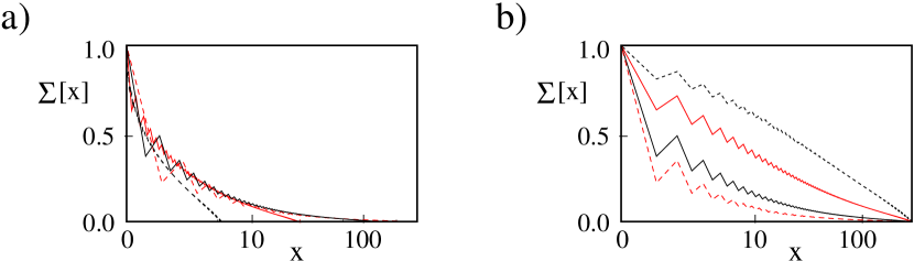
Figure 1:
a): Semilogarithmic rescaled curves for ${\bf\Sigma}[x]$ corresponding to $\ell=300$, $\Delta=0.3$ and, respectively, $J^{\prime}/J=0.1$ (dashed black curve), $J^{\prime}/J=0.2$ (full red curve), $J^{\prime}/J=0.4$ (full black curve), and $J^{\prime}/J=0.6$ (dashed red curve);
b): Same as in panel a), but without rescaling.

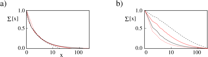
Figure 2:
a): Semilogarithmic rescaled curves for ${\bf\Sigma}[x]$ corresponding to $\ell=300$, $\Delta=-0.3$ and, respectively, $J^{\prime}/J=0.1$ (dashed black curve), $J^{\prime}/J=0.2$ (full red curve), $J^{\prime}/J=0.4$ (full black curve), and $J^{\prime}/J=0.6$ (dashed red curve);
b): Same as in panel a), but without rescaling.

${\rm Scaling\>factor}$	$\Delta=0.3$	$\Delta=-0.3$
$\frac{\xi_{K}[0.6,\Delta]}{\xi_{K}[0.4,\Delta]}$	0.4554	0.5662
$\frac{\xi_{K}[0.6,\Delta]}{\xi_{K}[0.2,\Delta]}$	0.0974	0.2006
$\frac{\xi_{K}[0.6,\Delta]}{\xi_{K}[0.1,\Delta]}$	0.0181	0.0676

Table 1: Scaling factors for $\Delta=0.3$ and $\Delta=-0.3$ and for $J^{\prime}/J=0.6,0.4,0.2,0.1$ evaluated using the scaling collapse technique.

An important observation about our method is that, differently from what has been done in Ref. [Holzner et al., 2009], we do not fit the ratios between the Kondo screening lengths from the numerical data. Instead, we compute them within perturbative RG approach and eventually find that the collapse of the curves is quite good after rescaling $x$ with the values we computed. In Fig. 1a), we see quite a good collapse of the curves onto each other for any value of $J^{\prime}/J$, but $J^{\prime}/J=0.1$. The lack of collapse in this last case can be traced back to a possible value of $\xi_{K}[0.1,0.3]$ exceeding the half-length of the chain ($\sim 300$). As we will show below, where we will be using a different technique allowing for directly estimating $\xi_{K}$, this is, in fact, the case, that shows the full consistency of our results with the expected Kondo scaling behavior. At variance, in Fig. 1b) we see a pretty good collapse of all the curves, implying that, in this case, all the Kondo screening lengths are $<300$, including $\xi_{K}[0.1,-0.3]$. In addition, due to the fact that the bulk spin correlations are now ferromagnetic ($\Delta<0$), the staggered component of the integrated spin correlations disappears, all the curves look quite smooth, as a function of $x$, and the corresponding collapse is even more evident than that of Fig. 1.

To ultimately fix the over-all factor in $\xi_{K}$, we now discuss the Kondo length collapse technique.

III.2 The Kondo length collapse technique

The Kondo length collapse technique (KLCT) is grounded on the “physical” meaning of the Kondo cloud as the cloud of spins fully screening ${\bf S}_{\bf G}$ into the Kondo singlet Sørensen and Affleck (1996). In the presence of a perfect screening, one would expect $\xi_{K}$ to emerge as the first zero of ${\bf\Sigma}[x]$ one meets when moving from the impurity location into the leads. In practice, as we discuss above, the actual zero of ${\bf\Sigma}[x]$ is set at $x=\ell$ by the over-all boundary conditions. Therefore, to extract $\xi_{K}$ one first of all sets a conventional “reduction factor” $r(<1)$ by defining a putative Kondo screening length $\xi_{K}^{(r)}$ as the value of $x$ at which ${\bf\Sigma}[x]$ is reduced by $r$ with respect to its value at $x=0$, that is, ${\bf\Sigma}[x=\xi_{k}^{(r)}]=r$. Choosing a specific value for $r$ is equivalent to fix $\ell_{0}$. Yet, variations around a reasonable choice of $r$ (such that basically all, or almost all, of the Kondo cloud resides over distances $\leq\xi_{K}^{(r)}$ from the impurity location) just affect the estimated value of $\xi_{K}^{(r)}$ by a factor of order 1 Holzner et al. (2009). Thus, in the following we choose to follow Ref. [Holzner et al., 2009], by choosing $r=0.1$ and accordingly using $\xi_{K}^{(0.1)}$ evaluated at given $\Delta$ and $J^{\prime}/J$ as an estimate of $\xi_{K}[J^{\prime}/J,\Delta]$. This eventually allows us to uniquely set $\ell_{0}$ and to provide the actual values of $\xi_{K}$ for various choices of the system parameters. In practice, at a given $\ell$, fixing $\Delta$ and $J^{\prime}/J$, one uses DMRG results to extract an $\ell$-dependent scale $\xi_{K}^{(0.1)}[J^{\prime}/J,\Delta,\ell]$ by means of the condition ${\bf\Sigma}[x=\xi_{K}^{(0.1)}[J^{\prime}/J,\Delta,\ell]]=0.1$. For large enough values of $\ell$, $\xi_{K}^{(0.1)}[J^{\prime}/J,\Delta,\ell]$ is expected to reach an asymptotic value $\xi_{K}^{(0.1)}[J^{\prime}/J,\Delta]$ which is independent of $\ell$ and, according to the above observations, provides the corresponding estimate of $\xi_{K}$. Based on these observations, in Fig. 3 we plot ${\bf\Sigma}[x]$ vs. $x$ on a semilogarithmic scale (on the $x$ axis), at $\Delta=0.3$ and, respectively, $J^{\prime}/J=0.6$ (Fig. 3a) ), $J^{\prime}/J=0.4$ (Fig. 3b) ), $J^{\prime}/J=0.2$ (Fig. 3c) ), $J^{\prime}/J=0.1$ (Fig. 3d) ). All the plots display curves corresponding to $\ell=50$ (dashed black curve), $\ell=100$ (solid red curve), $\ell=150$ (solid black curve),and $\ell=300$ (dashed red curve).

According to the discussion above, from Fig. 3a) and from Fig. 3b) we conclude that both $\xi_{K}[0.6,0.3]$ and $\xi_{K}[0.4,0.3]$ are $\ll 150$. In fact, a numerical estimate provides $\xi_{K}[0.6,0.3]\approx 10.23$ and $\xi_{K}[0.4,0.3]\approx 23.11$. At variance, the absence of collapse at ${\bf\Sigma}[x]=r$ for $J^{\prime}/J=0.1$ and $=0.2$ implies that in both cases $\xi_{K}$ must be comparable with (or larger than) $\ell=150$. Knowing the actual value of $\xi_{K}[0.6,0.3]$ allows us to estimate $\xi_{K}[0.2,0.3]$ and $\xi_{K}[0.1,0.3]$ by just using the scaling ratios derived in section III.1 within the SCT. The results are summarized in table 2. Apparently, they confirm the conclusion that both $\xi_{K}[0.2,0.3]$ and $\xi_{K}[0.1,0.3]$ are $>150$. The shorter values of the Kondo screening length at a given $J^{\prime}/J$ (compared to the ones at $\Delta=0.3$) allow us to directly estimate $\xi_{K}[J^{\prime}/J,-0.3]$ for $J^{\prime}/J=0.6,0.4,0.2$. This time, only $\xi_{K}[0.1,-0.3]$ had to be found using the corresponding scaling ratio derived in section III.1.

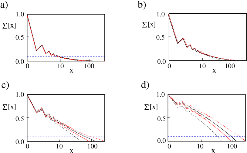
Figure 3:
a): Curves for ${\bf\Sigma}[x]$ at $\Delta=0.3$, $J^{\prime}/J=0.6$ and $\ell=50$ (dashed black curve), $\ell=100$ (solid red curve), $\ell=150$ (solid black curve), $\ell=300$ (dashed red curve). As a guide to the eye, the horizontal line at $y=0.1$ is shown as a dashed blue segment;
b): Same as in panel a), but for $J^{\prime}/J=0.4$;
c): Same as in panel a), but for $J^{\prime}/J=0.2$;
d): Same as in panel a), but for $J^{\prime}/J=0.1$.

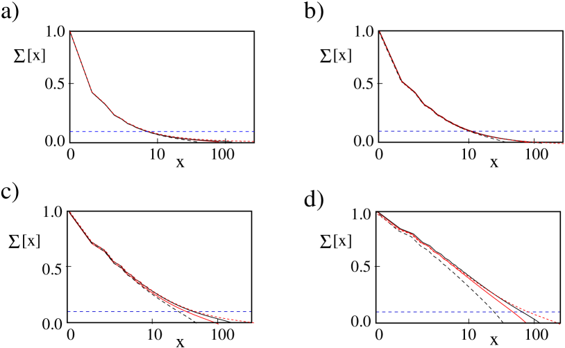
Figure 4:
a): Curves for ${\bf\Sigma}[x]$ at $\Delta=-0.3$, $J^{\prime}/J=0.6$ and $\ell=50$ (dashed black curve), $\ell=100$ (solid red curve), $\ell=150$ (solid black curve), $\ell=300$ (dashed red curve). As a guide to the eye, the horizontal line at $y=0.1$ is shown as a dashed blue segment;
b): Same as in panel a), but for $J^{\prime}/J=0.4$;
c): Same as in panel a), but for $J^{\prime}/J=0.2$;
d): Same as in panel a), but for $J^{\prime}/J=0.1$.

To stress the possibility of estimating some Kondo lengths by only combining the Kondo length collapse with the scaling collapse approach, in table 2 we report in black the values directly estimated using KLCT, in red the ones inferred combining KLCT with the results of section III.1 for the scaling factors.

$J^{\prime}/J$	$\xi_{K}[J^{\prime}/J,0.3]$	$\xi_{K}[J^{\prime}/J,-0.3]$
0.6	10.23	9.61
0.4	23.11	16.47
0.2	109.14	48.33
0.1	565.19	142.16

Table 2: Values for the Kondo length for $\Delta=0.3$ and $\Delta=-0.3$ and for $J^{\prime}/J=0.6,0.4,0.2,0.1$ evaluated using the KLCT (numbers displayed in black), or combining the KLCT with the SCT (numbers displayed in red).

As a general, concluding comment about KLCT, we note that, in order for the method to be effective, we need at least the two curves corresponding to the largest value of $\ell$ and to the next-to-largest one ($\ell^{{}^{\prime}}$) to collapse onto each other. Since this implies that both of them must not be affected by finite-size effect, we infer that the necessary condition for the collapse to happen is that $\xi_{K}\ll\ell^{{}^{\prime}}$, which motivates the absence of collapse in some of the plots in Fig. 3 and in Fig. 4. Of course, one could increase $\ell$ and directly estimate the value of $\xi_{K}$ from the collapse. Yet, for the sake of the presentation, we prefer to present some plots not showing collapse, in order to be able to discuss the main scenario and to show the remarkable consistency of the exact numerical data with the analytical results obtained within SLL framework, even for chains with a limited number of sites. Note that, after fitting the value of $\ell_{0}$ from DMRG results, the perturbative RG equations provide quite good estimates for $\xi_{K}[J^{\prime}/J,\Delta]$ and can be effectively used for such a purpose as, for instance, is was done in Ref. [Giuliano et al., 2017].

To conclude the discussion of the fully symmetric system, we now briefly comment on the behavior of ${\bf\Sigma}[x]$ outside of the Kondo cloud.

III.3 Kondo screening cloud in the XXZ spin chain

The way we apply SCT and KLCT to obtain $\xi_{K}$ from DMRG data relies upon the validity of Eq. (9) inside the Kondo cloud. Yet, based on very general grounds, a scaling form for ${\bf\Sigma}[x]$ such as the one in Eq. (9) is expected to apply outside of the Kondo cloud, as well, provided $x,\xi_{K}\ll\ell$ Sørensen and Affleck (1996); Barzykin and Affleck (1996, 1998) though, clearly, the perturbative RG estimate of the right-hand side of Eq. (9) and of Eq. (8), does no more apply. To pertinently replace Eq. (8) we need the analog, for our spin-chain model, of the conformal field theory based nonperturbative approach to Kondo screening cloud developed by Affleck and Ludwig Affleck and Ludwig (1991); Ludwig and Affleck (1994). To do so, we have to work out the analog, in our case, of Nozierès Fermi liquid theory Nozières (1974, 1978). In fact, in the spin chain framework, the analog of Nozierès Fermi liquid is the “healing” of the chain, that is, the saturation of the running couplings to values that are of the order of all the other bulk couplings Giuliano et al. (2017). In addition, the Kondo cloud emerges around ${\bf S}_{\bf G}$ of size $\sim 2\xi_{K}$. This can be roughly regarded as an extended region ${\cal R}$ embedded within the chain, which is coupled at its endpoints to the spins in the remaining part of the chain by means of the boundary Hamiltonian $H_{\rm SC}$, given by

$$H_{\rm SC}=J\{S_{\xi_{K},L}^{+}S_{\xi_{K}+1,L}^{-}+S_{\xi_{K},L}^{-}S_{\xi_{K}+1,L}^{+}+\Delta S_{\xi_{K},L}^{z}S_{\xi_{K}+1,L}^{z}\}+J\{S_{\xi_{K},R}^{+}S_{\xi_{K}+1,R}^{-}+S_{\xi_{K},R}^{-}S_{\xi_{K}+1,R}^{+}+\Delta S_{\xi_{K},R}^{z}S_{\xi_{K}+1,R}^{z}\}\,.$$ (11)

Regarding the Kondo cloud as a spin-singlet spin cluster of size $\sim 2\xi_{K}$ coupled to two spin chains at its endpoints allows to employ a pertinent generalization of the derivation in appendix A.2 to recover the behavior of ${\bf\Sigma}[x]$ for $x>\xi_{K}$. First, we note that, due to the boundary condition ${\bf\Sigma}[\ell]=0$, we may equivalently set

$${\bf\Sigma}[x]=-\sum_{i=x+1}^{\ell}\sum_{X=L,R}\left\{\frac{\langle S_{\bf G}^{z}S_{i,X}^{z}\rangle-\langle S_{\bf G}^{z}\rangle\langle S_{i,X}^{z}\rangle}{\langle(S_{\bf G}^{z})^{2}\rangle-(\langle S_{\bf G}^{z}\rangle)^{2}}\right\}\,.$$ (12)

Therefore, we see that, due to strong singlet correlations within the Kondo cloud, one may legitimately approximate the whole chain ground state as $|\Psi\rangle_{0}=|{\rm KC}\rangle\otimes|{\bf 0}\rangle_{L}\otimes|{\bf 0}\rangle_{R}$, with $|{\rm KC}\rangle$ being the “Kondo cloud spin singlet ground state” and $|{\bf 0}\rangle_{L}$ and $|{\bf 0}\rangle_{R}$ respectively being the ground states of the portion of the _L and of the _R spin chain ranging from $\xi_{K}+1$ to $\ell$. Therefore, due to the singlet nature of $|{\rm KC}\rangle$, one obtains $\langle\Psi_{0}|S_{\bf G}^{z}S_{j,L(R)}^{z}|\Psi_{0}\rangle=0$ whenever $j>\xi_{K}$. Accordingly, to estimate the leading nonzero contribution to the correlation function, one has to correct the system’s ground state from $|\Psi_{0}\rangle$ to a state $|\Psi_{1}\rangle$ taking into account the effects of $H_{\rm SC}$ in Eq. (11). To leading order, one obtains

$$|\Psi_{1}\rangle\approx|\Psi\rangle_{0}-\left\{J\Delta S_{\xi_{K}+1,L}^{z}\sum_{X}\>|X\rangle\frac{\langle X|S_{\xi_{K},L}|\Psi\rangle_{0}}{\delta E_{X}}+J\Delta S_{\xi_{K}+1,R}^{z}\sum_{X}\>|X\rangle\frac{\langle X|S_{\xi_{K},R}|\Psi\rangle_{0}}{\delta E_{X}}\right\}\otimes|{\bf 0}\rangle_{L}\otimes|{\bf 0}\rangle_{R}\,,$$ (13)

with the sum at the right-hand side of Eq. (13) taken over low-lying excited states of the Kondo cloud spin singlet, $\{|X\rangle\}$, with corresponding excitation energy $\delta E_{X}$ (measured with respect to the ground state). As a result, to leading order in $H^{\prime}$, one obtains for $j>\xi_{K}$

$$\frac{\langle\Psi_{1}|S_{\bf G}^{z}S_{j,L(R)}^{z}|\Psi_{1}\rangle-\langle\Psi_{1}|S_{\bf G}^{z}|\Psi_{1}\rangle\langle\Psi_{1}|S_{j,L(R)}^{z}|\Psi_{1}\rangle}{\langle\Psi_{1}|(S_{\bf G}^{z})^{2}|\Psi_{1}\rangle-(\langle\Psi_{1}|S_{\bf G}^{z}|\Psi_{1}\rangle)^{2}}\approx$$

$$-J\Delta\sum_{X}\left\{\frac{\langle\Psi_{0}|S_{\xi_{K},L(R)}^{z}|X\rangle\langle X|S_{\bf G}^{z}|\Psi_{0}\rangle}{\delta E_{X}}\right\}\>_{L(R)}\langle{\bf 0}|S_{\xi_{K}+1,L(R)}^{z}S_{j,L(R)}^{z}|{\bf 0}\rangle_{L(R)}\,.$$ (14)

To compute the correlation functions ${}_{L(R)}\langle{\bf 0}|S_{\xi_{K}+1,L(R)}^{z}S_{j,L(R)}^{z}|{\bf 0}\rangle_{L(R)}$, we use the result for the homogeneous open XXZ chain, Eq. (49), by substituting $\ell$ with $\hat{\ell}=\ell-\xi_{K}$ and $x$ with $\hat{j}=j-\xi_{k}$. As a result, we therefore conclude that these correlation functions are independent of $\xi_{K}$ up to terms $\propto(\xi_{K}/\ell)\ll 1$. Moreover, at a given $|X\rangle$, the matrix element $\langle X|S_{j}^{z}|\Psi_{0}\rangle$ is poorly dependent on $j$, as long as the spin ${\bf S}_{j}$ lies within the Kondo cloud. Since one expects $\delta E_{X}\sim\xi_{K}^{-1}$, we eventually combine Eqs. (12, 13, 14) to conclude that, for $x>\xi_{K}$, one obtains

$${\bf\Sigma}[x]\approx\xi_{K}\sum_{\bar{d}_{b}}\>\ell^{\bar{d}_{b}}\>\omega_{\bar{d}_{b}}\left(\frac{x}{\ell}\right)+\ldots\,,$$ (15)

with the sum taken over a pertinent set of scaling exponents and the ellipses standing for additional contributions $\propto\xi_{K}/\ell$, which we neglect, due to the assumed condition $\xi_{K}/\ell\ll 1$. For instance, from Eq. (49), we infer that, for $\xi_{K}\ll x\ll\ell$, one obtains

$$\sum_{\bar{d}_{b}}\>\ell^{\bar{d}_{b}}\>\omega_{\bar{d}_{b}}\left(\frac{x}{\ell}\right)\approx-\frac{g}{2\ell^{2}}\>\sum_{j=x+1}^{\ell}\left[\frac{1}{1-\cos\left(\frac{\pi j}{\ell}\right)}\right]-\frac{2ag}{\ell}\>\sum_{j=x+1}^{\ell}\left[(-1)^{j}\>\left|\frac{2\ell}{\pi}\sin\left(\frac{\pi j}{\ell}\right)\right|^{-g}\cot\left(\frac{\pi j}{2\ell}\right)\right]\,.$$ (16)

As a result, we expect that, when synoptically considering plots of ${\bf\Sigma}[x]$ derived at different values of $J^{\prime}/J$ (that is, of $\xi_{K}$), with $x$ lying outside of the Kondo cloud, the curves collapse onto each other, provided ${\bf\Sigma}[x]$ is rescaled to $\hat{\bf\Sigma}[x]=\xi_{K}^{-1}{\bf\Sigma}[x]$, which incidentally appears to be consistent with Affleck-Ludwig result for the real-space correlations at $x$ lying outside of the Kondo cloud Affleck and Ludwig (1991); Ludwig and Affleck (1994).

To check this result, in Fig. 5 we plot curves for $\hat{\bf\Sigma}[x]$ for $\Delta=0.3$ and $J^{\prime}/J=0.2,0.4,0.6$ (Fig. 5a)), and for $\Delta=-0.3$ and the same values of $J^{\prime}/J$ (Fig. 5b)). In drawing the plots, we rescaled the various curves with the ratios between the corresponding Kondo screening lengths, as derived in Sec.III.1. In the two plots, the dashed red curve and the solid black curve respectively correspond to $J^{\prime}/J=0.6$ and $J^{\prime}/J=0.4$. We see that, both for $\Delta=0.3$ and for $\Delta=-0.3$, the two curves collapse onto each other for $x>\xi_{K}[0.4,\Delta]$. Moreover, in both plots we note that the solid red curve (corresponding to $J^{\prime}/J=0.2$) collapses onto the other two ones for $x>\xi_{K}[0.2,\Delta]$. This remarkable result is consistent with the discussion provided above and constitutes another direct evidence for the emergence of the Kondo cloud over a length scale $\sim\xi_{K}$.

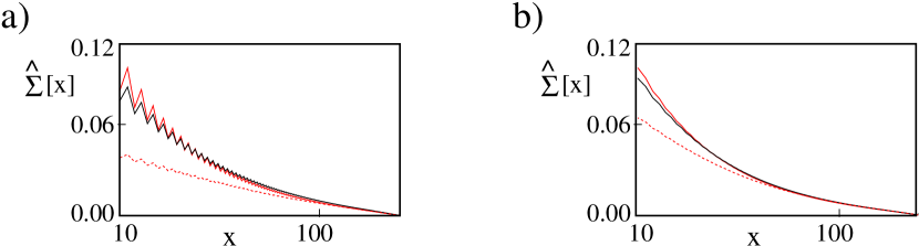
Figure 5:
a): Rescaled curves (see main text) for $\hat{\bf\Sigma}[x]$ at $\Delta=0.3$, $J^{\prime}/J=0.6$ and $\ell=300$ (dashed red curve), $J^{\prime}/J=0.4$ (solid black curve), and $J^{\prime}/J=0.2$ (solid red curve). There is an apparent collapse of the first two curves onto each other for $x>\xi_{K}[0.4,0.3]$ and of all three curves onto each other for $x>\xi_{K}[0.2,0.3]$; b): Same as in panel a), but for $\Delta=-0.3$.

We now move to discuss models in which either the _L-_R-symmetry in the Kondo couplings, or the spin-parity symmetry (or both) are broken and see how the lack of those symmetry affects the main picture for the Kondo cloud we derived so far.

IV Non symmetric Kondo interaction Hamiltonian

In this section we discuss how Kondo effect is affected by either a breaking of the symmetry between the couplings of ${\bf S}_{\bf G}$ to the two leads, or by the onset of a nonzero $B$ (or both), starting with the asymmetry in the couplings to the leads.

IV.1 Magnetic impurity with asymmetric Kondo couplings

To discuss the effects of asymmetries in the Kondo couplings, here we assume that, in ${\cal H}$ in Eq. (1), we have $J_{L}^{{}^{\prime}}<J_{R}^{{}^{\prime}}$ and $J_{z,L(R)}^{{}^{\prime}}=\Delta J_{L(R)}^{{}^{\prime}}$, which eventually implies $J_{z,L}^{{}^{\prime}}<J_{z,R}^{{}^{\prime}}$, as well. According to the discussion of section III.2 we again expect a Kondo cloud to emerge, with $\xi_{K}=\xi_{K,R}$, that is, $\xi_{K}$ is set by the stronger coupling of ${\bf S}_{\bf G}$, while the weaker coupling leads to the residual Hamiltonian $H_{W}$ in Eq. (4). As stated in section III.2, $H_{W}$ does not lead to an additional dynamical length scale. In fact, it merely affects the value of $\xi_{K}$ by continuously renormalizing it from what one would have for just a magnetic impurity Kondo-coupled at the endpoint of a single XXZ chain Eggert and Affleck (1992), to the value one obtains in the case of symmetric couplings. Note that the dependence of $\xi_{K}$ on the (stronger) Kondo coupling strength can be readily inferred from Eqs. (52), which, just as in the symmetric case, fixes the screening length, up to an over-all factor. The latter carries information on how the screening is distributed throughout the two channels and, in general, it can hardly be recovered within SLL-based perturbative RG approach. Thus, in the following we directly determine it from numerical DMRG data. Specifically, to spell this point out, we define integrated correlation functions at both sides of ${\bf S}_{\bf G}$, ${\bf\Sigma}_{L,R}[x]$, both depending on a parameter $\chi$, so that

$${\bf\Sigma}_{L}[x] = \chi+\sum_{j=1}^{x}\left\{\frac{\langle S_{\bf G}^{z}S_{j,L}^{z}\rangle-\langle S_{\bf G}^{z}\rangle\langle S_{j,L}^{z}\rangle}{\langle(S_{\bf G}^{z})^{2}\rangle-(\langle S_{\bf G}^{z}\rangle)^{2}}\right\}\,,$$

$${\bf\Sigma}_{R}[x] = 1-\chi+\sum_{j=1}^{x}\left\{\frac{\langle S_{\bf G}^{z}S_{j,R}^{z}\rangle-\langle S_{\bf G}^{z}\rangle\langle S_{j,R}^{z}\rangle}{\langle(S_{\bf G}^{z})^{2}\rangle-(\langle S_{\bf G}^{z}\rangle)^{2}}\right\}\,.$$ (17)

By definition, from Eq. (17) one has ${\bf\Sigma}[x]={\bf\Sigma}_{L}[x]+{\bf\Sigma}_{R}[x]$, which implies the boundary condition ${\bf\Sigma}[\ell]={\bf\Sigma}_{L}[\ell]+{\bf\Sigma}_{R}[\ell]=0$. In addition, to fix $\chi$ we explicitly require that both integrated correlation functions are vanishing at $x=\ell$, that is, ${\bf\Sigma}_{L}[\ell]={\bf\Sigma}_{R}[\ell]=0$. Doing so, we roughly state that the Kondo cloud is, in general, non symmetrically distributed across the leads and is such that the part at the right(left)-hand side lead screens the impurity by a fraction equal to $1-\chi$ ($\chi$). Apparently, one has $0\leq\chi\leq 1$ and, varying $\chi$, one can continuously move from the two-channel Kondo regime we studied in section III, corresponding to $\chi=1/2$, in which the Kondo cloud is symmetrically distributed over the two leads, to the perfect one-channel Kondo regime, either corresponding to $\chi=0$, or to $\chi=1$, in which the Kondo cloud is fully distributed over one lead only. $\chi$ appears to be a smooth function interpolating between the values 0 (at $J^{\prime}_{L}/J_{R}^{{}^{\prime}}=0$) and $1$ (at $J^{\prime}_{L}/J_{R}^{{}^{\prime}}\to\infty$), and equal to $1/2$ at $J^{\prime}_{L}/J_{R}^{{}^{\prime}}=1$. We also have $\chi<(>)1/2$ according to whether $J_{L}^{{}^{\prime}}<(>)J_{R}^{{}^{\prime}}$, which implies that the lead that actually sets $\xi_{K}$ has to screen an impurity effectively larger by $1/2-\chi$ ($\chi-1/2$) than what it would be at the symmetric point. Eventually, this shows us the rationale of introducing Eqs. (17), that is, that any asymmetry between the Kondo couplings must imply an increase in $\xi_{K}$ with respect to the value it takes at the symmetric point. To check our prediction, in the following we estimate $\xi_{K}$ and $\xi_{K,R}$ for $\Delta=0.3$, $J^{{}^{\prime}}_{R}=0.6$, $J_{z,L(R)}^{{}^{\prime}}=\Delta J_{L(R)}^{{}^{\prime}}$, and $J^{{}^{\prime}}_{L}/J=0.6,0.4,0.2$ (note that our choice for $J^{{}^{\prime}}_{R}/J$ is expected, based on the results of the previous sections, to make $\xi_{K}$ of the order of 10 lattice spacings, which allows us to make reliable simulations using chain with at most 300 sites at each side of ${\bf S}_{\bf G}$). To estimate $\xi_{K}$, we used KLCT at $J^{{}^{\prime}}_{L}/J=0.4,0.2$. In Fig. 6, we show the collapse of the curves for ${\bf\Sigma}[x]$ derived at $\ell=50,100,150,300$. The estimated values of $\xi_{K}$ are reported in table 3.

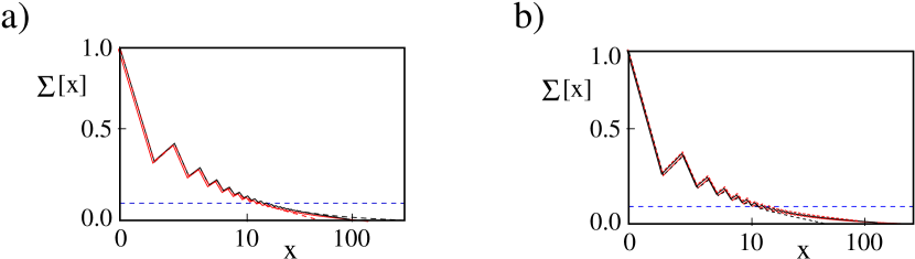
Figure 6:
a): Curves for ${\bf\Sigma}[x]$ at $\Delta=0.3$, $J_{R}^{{}^{\prime}}/J=0.6$, $J_{L}^{{}^{\prime}}/J=0.4$, and $\ell=50$ (dashed black curve), $\ell=100$ (solid red curve), $\ell=150$ (solid black curve), $\ell=300$ (dashed red curve). As a guide to the eye, the horizontal line at $y=0.1$ is shown as a dashed blue segment;
b): Same as in panel a), but for $J_{L}^{{}^{\prime}}/J=0.2$.

Next, we estimate the parameter $\chi$ in the three cases we consider. To do so, we just consider the value of the function $\tilde{\bf\Sigma}[x]=1+\sum_{j=1}^{x}\left\{\frac{\langle S_{\bf G}^{z}S_{j,R}^{z}\rangle-\langle S_{\bf G}^{z}\rangle\langle S_{j,R}^{z}\rangle}{\langle(S_{\bf G}^{z})^{2}\rangle-(\langle S_{\bf G}^{z}\rangle)^{2}}\right\}$ at $x$ equal to the largest available value from simulations, $x=\ell=300$. From the plots of $\tilde{\bf\Sigma}[x]$ reported in Fig. 7, we extract the values of $\chi$ reported in table 3. At a given value of $J_{L}^{{}^{\prime}}/J$, once $\chi$ is determined as discussed above, we extract $\xi_{K,R}$ by applying the KLTC to the function ${\bf\Sigma}_{R}[x]$ defined in Eq. (17) and plotted in Fig.8.

The results, reported in the last column of table 3, have an excellent consistency with the ones obtained for $\xi_{K}$ at the same values of $J_{L}^{{}^{\prime}}/J$. This ultimately confirms our prediction that the $\xi_{K}$ can be determined by assuming that the right-hand lead (the one feeling the stronger coupling to the impurity) screens an effective impurity larger by $1/2-\chi$ than that would be at the symmetric point. In addition, we verify that, as expected, the residual weak-link interaction in Eq. (4) does not induce any additional length scale associated with screening Rommer and Eggert (2000). To do so, we resorted to SCT and plotted the curves for ${\bf\Sigma}[x]$ computed at $\Delta=0.3$, $J^{\prime}_{R}/J=0.6$ and at $J^{{}^{\prime}}_{L}/J=0.6,0.4,0.2$ and for $\ell=300$ by rescaling the $x$ coordinate with the ratio between the corresponding $\xi_{K}$ and the $\xi_{K}$ computed at $J^{{}^{\prime}}_{L}/J=0.6$ (result of table 3). We plot the result in Fig. 9a) where, for comparison, we also plot the same curves drawn without rescaling $x$ (Fig. 9b)). Apparently, the excellent collapse in Fig. 9a) evidences that no length scales but $\xi_{K}=\xi_{K,R}$ are dynamically generated by Kondo interaction.

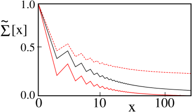
Figure 7: Curves for $\tilde{\bf\Sigma}[x]$ vs. $x$ at $\Delta=0.3$, $J_{R}^{{}^{\prime}}/J=0.6$, $\ell=300$, $J_{L}^{{}^{\prime}}/J=0.4$ (solid red curve), and $J_{L}^{{}^{\prime}}/J=0.2$ (solid black curve). The estimated value of $\chi$ (see text) is $\chi=0.238$ in the former case, $\chi=0.055$ in the latter case.

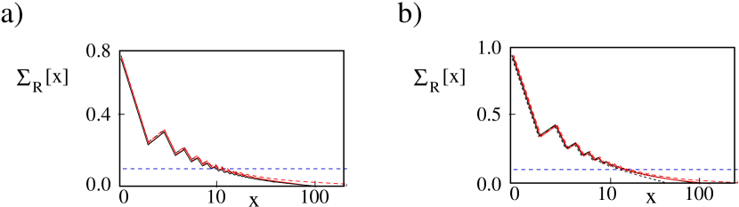
Figure 8:
a): Curves for ${\bf\Sigma}_{R}[x]$ at $\Delta=0.3$, $J_{R}^{{}^{\prime}}/J=0.6$, $J_{L}^{{}^{\prime}}/J=0.4$, and $\ell=50$ (dashed black curve), $\ell=100$ (solid red curve), $\ell=150$ (solid black curve), $\ell=300$ (dashed red curve). As a guide to the eye, the horizontal line at $y=0.1$ is shown as a dashed blue segment;
b): Same as in panel a), but for $J_{L}^{{}^{\prime}}/J=0.2$.

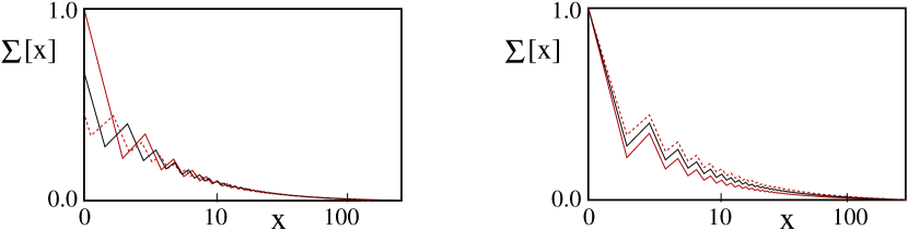
Figure 9:
a): Curves for ${\bf\Sigma}[x]$ at $\Delta=0.3$, $\ell=300$, $J_{R}^{{}^{\prime}}/J=0.6$ and $J_{L}^{{}^{\prime}}/J=0.6$ (red dashed curve), $J_{L}^{{}^{\prime}}/J=0.4$ (black solid curve), and $J_{L}^{{}^{\prime}}/J=0.2$ (black solid curve): here the $x$ coordinate is rescaled with the ratio between the corresponding screening length, to induce curve collapse;
b): Same as in panel a), but without rescaling $x$.

$J^{{}^{\prime}}_{L}/J$ (at $J_{R}^{{}^{\prime}}/J=0.6$)	Parameter $\chi$	$\xi_{K}$ (from ${\bf\Sigma}[x]$)	$\xi_{K,R}$ (from ${\bf\Sigma}_{R}[x]$)
$0.6$	$0.5$	$10.23$	$10.23$
$0.4$	$0.238$	$14.07$	$13.87$
$0.2$	$0.055$	$18.13$	$17.98$

Table 3: Estimated values of the parameter $\chi$ (from Fig. 7), of $\xi_{K}$ (from Fig. 6) and of $\xi_{K,R}$ (from Fig. 8) for $J^{\prime}_{R}/J=0.6$ and $J^{{}^{\prime}}_{L}/J=0.6,0.4,0.2$.

To summarize, we may conclude that, for a magnetic impurity in an XXZ-chain, an _L-_R asymmetry in the Kondo couplings does not spoil Kondo effect, as evidenced by scaling properties of the ${\bf\Sigma}[x]$. However, it takes some important consequences in that it affects the distribution of the net screening between the leads, ultimately resulting in a renormalization of $\xi_{K}$ which, as a function of the weaker coupling, continuously evolves from the value it takes in the two-channel case (symmetric coupling), to the value it takes in the one-channel case (weaker coupling set to $0$) Eggert and Affleck (1992). Conversely, on keeping $J_{L}^{{}^{\prime}}$ fixed and increasing $J_{R}^{{}^{\prime}}$, we expect a continuous shrinking of $\xi_{K}$. Eventually, when $J_{R}^{{}^{\prime}}=J$, the right-hand lead plus ${\bf S}_{\bf G}$ turns into an uniform $\ell+1$-site chain, coupled to the $\ell$-site left-hand lead via the weak-link Hamiltonian with parameters $J_{L}^{{}^{\prime}},J_{z,L}^{{}^{\prime}}$. This suggests a first mean to experimentally trigger the crossover from Kondo effect to weak-link regime by continuously increasing $J_{R}^{{}^{\prime}}$ till it becomes equal to $J$. At the same time, the expected continuous shrinking of $\xi_{K}$ makes it eventually become of the order of the lattice site, which is appropriate when the onset of the weak link regime suppresses the scaling with $\xi_{K}$.

IV.2 Nonzero applied magnetic field

We now discuss the effects of a nonzero $B$ at the impurity site, i.e., the last term in Eq. (1) on the Kondo screening and on the consequent value of $\xi_{K}$. In general, in the context of an XXZ spin chain, the effect of a finite uniform magnetic field in the $z$-direction can be accounted for by pertinently modifying the SLL approach Hikihara and Furusaki (2004), which proves that a uniform field only qualitatively affects Kondo effect at the impurity. Also, when regarding the XXZ chain as an effective description of the Bose-Hubbard model, a uniform magnetic field arises from a uniform deviation of half-filling in the chemical potential of the Bose-Hubbard model which, again, does not qualitatively affect the system’s behavior, at least as long as one works at finite particle number in the Bose-Hubbard model (canonical ensemble), corresponding to fixed $z$-component of the total spin in the XXZ chain Giuliano et al. (2013, 2017).

In the context of electronic Kondo effect, a nonzero $B$ has shown to result in a splitting in the Kondo resonance (with respect to the electron spin) that sets in at values of $B$ comparable with $T_{K}$. This comes together with a substantial suppression of the magnetoresistance/magnetoconductance across the Kondo impurity Costi (2000); Otte et al. (2008). As for what concerns the effects of a nonzero $B$ at an impurity in a spin chain, to the best of our knowledge there is no, so far, a systematic study of how $B$ affects $\xi_{K}$ and, more in general, the development of the Kondo cloud. We now investigate this point by means of a combined use of the perturbative RG approach, based on the finite-$B$ RG equations in Eqs. (52), and on DMRG approach to estimate $\xi_{K}$ at given values of the system parameters.

Within perturbative RG approach, we integrate Eqs. (52) (which are expected to rigorously apply in the small-$B$ limit, that is, for $B/J\ll 1$), and use the integrated curves to define a “generalized” Kondo length, $\xi_{K}[J^{\prime}/J,\Delta,B/J]$, to be the scale at which the running couplings enter the nonperturbative regime, at given $J^{\prime},\Delta$ and $B$ (an important point to stress here is that, strictly speaking, $\xi_{K}[J^{\prime}/J,\Delta,B/J]$ can be regarded as an actual Kondo length only as long as Kondo effect is not suppressed by $B$, that is, for $B<T_{K}$. At larger values of $B$, Kondo effect gets suppressed by Zeeman energy Costi (2000), no Kondo length is dynamically generated though, still, $\xi_{K}[J^{\prime}/J,\Delta,B/J]$ keeps its meaning as over-all length scale of the system). On numerically integrating Eqs. (52) we draw plots of $\xi_{K}[J^{\prime}/J,\Delta,B/J]$ vs. $B$ at fixed $J^{\prime}/J$ and $\Delta$. In Fig. 10 we plot $\xi_{K}[J^{\prime}/J,\Delta,B/J]$ vs. $B/J$ evaluated at $\Delta=0.3$ and $J^{\prime}/J=0.6,0.4,0.3,0.2$, after rescaling the values of $\xi_{K}$ taking into account the numerical value of the overall scale in the Kondo length evaluated with the KLCT. While the curves should actually be trusted only at small values of $B/J$, it is interesting to attempt to draw some qualitative conclusions by looking at a window of values of $B/J$ ranging from $0$ to $2$, which is what we do in Fig. 10. The main trend of all the plotted curves is a decrease in $\xi_{K}$ at small values of $B/J$ followed by a remarkable collapse of all the various $\xi_{K}$’s onto a single value, of the order of a few lattice step, as $B/J\sim 1$. To account for such a behavior, we observe that a nonzero $B$ introduces an additional “magnetic” length scale in the problem, $\xi_{B}=\alpha J/B$, with $\alpha$ being a numerical factor of the order $1$, which we estimate later on from DMRG data. Accordingly, in employing the scaling approach, one has to properly modify Eq. (9), consistently with what is done in Ref. [Holzner et al., 2009] for the Anderson impurity in an otherwise noninteracting electron chain. This eventually leads to a two-parameter scaling behavior, that is, by denoting with ${\bf\Sigma}_{B}[x]$ the integrated spin correlation function at a nonzero $B$, we generalize Eq. (9) as

$${\bf\Sigma}_{B}[x]=\sum_{\bar{d}_{b}}\ell^{\bar{d}_{b}}\xi_{\bar{d}_{b}}\left[\frac{\xi_{K}}{\ell};\frac{\xi_{K}}{\xi_{B}};\frac{x}{\xi_{K}}\right]\,,$$ (18)

with, again, the sum taken over the scaling dimensions of the boundary operators entering the SLL representation for the XXZ spin chain with the local spin-1/2 impurity (note that in Eq. (18) we used $\bar{d}_{b}$ to denote a generic scaling dimension of a relevant boundary operator: using a different symbol from Eq. (9) is motivated by the observation that, in principle, a nonzero $B$ breaks symmetries such as, for instance, spin-parity, thus potentially allowing the emergence of relevant boundary operators which were forbidden by symmetry at $B=0$). To keep consistent with the zero-$B$ limit, as “initial condition” of Eq. (18) we require that

$$\sum_{\bar{d}_{b}}\ell^{\bar{d}_{b}}\xi_{\bar{d}_{b}}\left[\frac{\xi_{K}}{\ell};0;\frac{x}{\xi_{K}}\right]=\sum_{d_{b}}\ell^{d_{b}}\xi_{d_{b}}\left[\frac{\xi_{K}}{\ell};\frac{x}{\xi_{K}}\right]={\bf\Sigma}[x]\,.$$ (19)

From Eq. (19) we see that at small, but finite, values of $B/J$, ${\bf\Sigma}[x]$ is modified by a term $\propto B\xi_{K}$ with respect to its value at $B=0$, and so does $\xi_{K}$, as well. Moreover, a finite $B$ polarizes ${\bf S}_{\bf G}$, so to break the ${\bf S}_{\bf G}\to-{\bf S}_{\bf G}$-symmetry in the system Hamiltonian. The net average (“static”) polarization of ${\bf S}_{\bf G}$ corresponds to a reduction in the fluctuation of the local impurity spin. Since the finite extension of $\xi_{K}$ is a consequence of the dynamical mechanism of Kondo screening (related to the fluctuations in ${\bf S}_{\bf G}$), the smaller the fluctuations are, the less spins are needed to dynamically screen the impurity spin. Therefore, one naturally expects that a nonzero $B$ implies a reduction in $\xi_{K}$, as it appears from the plots in Fig. 10. This can be ultimately inferred from Eq. (19) taken in the limit $\xi_{K},\xi_{B},x\ll\ell$, required to suppress finite-size corrections to scaling, and $\xi_{B}\gg\xi_{K}$, corresponding to small values of $B$. In this limit, $\xi_{K}$ works as a reference length scale, and Eq. (18) simplifies into

$${\bf\Sigma}_{B}[x]\approx\hat{\bf\Sigma}_{1,B}[x]=\sum_{\bar{d}_{b}}\ell^{\bar{d}_{b}}\xi_{\bar{d}_{b}}\left[0;\frac{\xi_{B}}{\xi_{K}};\frac{x}{\xi_{K}}\right]\,.$$ (20)

Eq. (20) determines $\xi_{K}[J^{\prime}/J,\Delta,B/J]$ from the KLCT condition

$$\sum_{\bar{d}_{b}}\ell^{\bar{d}_{b}}\xi_{\bar{d}_{b}}\left[0;\frac{\xi_{B}}{\xi_{K}[J^{\prime}/J,\Delta]};\frac{\xi_{K}[J^{\prime}/J,\Delta,B/J]}{\xi_{K}[J^{\prime}/J,\Delta]}\right]=r\,,$$ (21)

where we choose $r=0.1$. Increasing $B$ from $B$ to $B^{\prime}=\rho B$ ($\rho>1$), we therefore obtain

$$\sum_{\bar{d}_{b}}\ell^{\bar{d}_{b}}\xi_{\bar{d}_{b}}\left[0;\frac{\xi_{B^{\prime}}}{\rho\xi_{K}[J^{\prime}/J,\Delta]};\frac{\rho\xi_{K}[J^{\prime}/J,\Delta,B^{\prime}/J]}{\rho\xi_{K}[J^{\prime}/J,\Delta]}\right]=\sum_{\bar{d}_{b}}\ell^{\bar{d}_{b}}\xi_{\bar{d}_{b}}\left[0;\frac{\xi_{B}}{\xi_{K}[J^{\prime}/J,\Delta]};\frac{\xi_{K}[J^{\prime}/J,\Delta,B/J]}{\xi_{K}[J^{\prime}/J,\Delta]}\right]\,,$$ (22)

which implies a reduction of $\xi_{K}[J^{\prime}/J,\Delta,B^{\prime}/J]$ by a factor $\rho^{-1}=B/B^{\prime}$. To check this conclusion, we compare the values of $\xi_{K}[J^{\prime}/J,\Delta,B/J]$ obtained from the integrated Eqs. (52) at $J^{\prime}/J=0.6$ and $\Delta=0.3$ as a function of $B/J$ with the estimates we derive by applying the KLCT to the DMRG results at the same values of $J^{\prime}/J$ and $\Delta$ and at the selected values of $B/J$. Note that, in order to enhance the window of expected validity of Eqs. (52), we have chosen the largest possible value of $J^{\prime}/J$ among the ones we consider in this work, so to minimize the corresponding value of $\xi_{K}$). In Fig. 11, we plot $\xi_{K}[0.6,0.3,B/J]$ vs. $B/J$ derived from Eqs. (52) for $0\leq B/J\leq 0.18$, and we display as black dots the values of $\xi_{K}[0.6,0.3,B/J]$ estimated within the Kondo length collapse technique applied to the DMRG results for $B/J=0.0,0.04,0.1,0.16$. We see that the dots lie quite close to the curve for $B/J\leq 0.1$, so, we infer a validity of the analytical RG Eqs. (52) for values of $B$ less or equal to ten percent of the high-energy cutoff ($\sim J$). Beyond those values of $B/J$, we may extrapolate that the DMRG results are systematically larger than the predictions of the perturbative RG approach, which is consistent with the fact that the latter technique systematically underestimates higher-order fluctuations, that are ultimately responsible for the size of the Kondo cloud Vladár and Zawadowski (1983a, b, c).

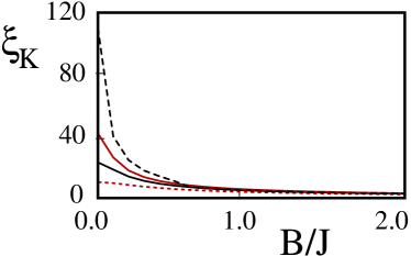
Figure 10: $\xi_{K}[J^{\prime}/J,\Delta,B/J]$ vs. $B/J$ derived from the integral curves corresponding to Eqs. (52) for $\Delta=0.3$ and $J^{\prime}/J=0.6$ (dashed red curve), $J^{\prime}/J=0.4$ (solid black curve), $J^{\prime}/J=0.3$ (solid red curve), and $J^{\prime}/J=0.2$ (dashed black curve).

Figure 11:
Solid red curve: $\xi_{K}[J^{\prime}/J,\Delta,B/J]$ vs. $B/J$ derived for $J^{\prime}/J=0.6$ and $\Delta=0.3$ from the integral curves corresponding to Eqs. (52).
Black dots: $\xi_{K}[J^{\prime}/J,\Delta,B/J]$ vs. $B/J$ derived for $J^{\prime}/J=0.6$ and $\Delta=0.3$ by applying Kondo length collapse approach to the DMRG results obtained for $B/J=0.0,0.04,0.1,0.16$.

The second remarkable feature shown in Fig. 10 is that increasing $B$ all the $\xi_{K}$’s collapse onto a single value, of the order of a few lattice steps. To understand this, we note that, as $B/J\sim 1$ and, accordingly, $\xi_{B}\ll\xi_{K}$, Eq. (18) simplifies into

$${\bf\Sigma}_{B}[x]\approx\hat{\bf\Sigma}_{2,B}[x]=\lim_{y\to\infty}\sum_{\bar{d}_{b}}\ell^{\bar{d}_{b}}\xi_{\bar{d}_{b}}\left[0;y;\frac{x}{\xi_{B}}\right]\,.$$ (23)

Eq. (23) again displays an universal scaling function, but now scaling with $\xi_{B}$ being the reference length scale, since any reference to the value of $J^{\prime}/J$ has disappeared. This eventually accounts for the collapse of all the Kondo lengths onto a $J^{\prime}$-independent value, at large enough values of $B$. To confirm this result with our numerical analysis, we applied KLCT to DMRG data for ${\bf\Sigma}[x]$ derived at $\ell=300$ for $J^{\prime}/J=0.2,0.3,0.4,0.6$ at $B/J=0.0,0.6,1.4,2.0$. We plot our result in Fig. 12, from which we see that, as soon as $B/J$ takes off, a remarkable collapse of the scaling lengths at various values of $J^{\prime}/J$ sets in (note that this also allows us to estimate $\alpha\approx 3.5$). In Fig. 12 we ultimately see an evident large-$B$ collapse, as predicted by Eqs. (52), though up to an over-all numerical factor.

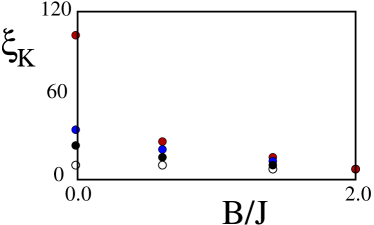
Figure 12: $\xi_{K}[J^{\prime}/J,\Delta,B/J]$ vs. $B/J$ derived for $\Delta=0.3$ by applying KLCT to the DMRG results obtained for $J^{\prime}/J=0.2$ (full red dots), $J^{\prime}/J=0.4$ (full blue dots), $J^{\prime}/J=0.3$ (full black dots), $J^{\prime}/J=0.6$ (empty dots), at $B/J=0.0,0.6,1.4,2.0$.

To conclude this section, a comment is in order about the possibility of using $B$ as a control parameter to drive the system along a crossover from a Kondo-like behavior to a weak-link like behavior. We note that, in the $B/J\gg 1$-limit, one of the two impurity levels is pushed very high in energy, with respect to the other one. This strongly suppresses processes in which ${\bf S}_{\bf G}$ switches between the two eigenstates of $S_{\bf G}^{z}$, leaving them only as virtual processes. To take this into account, one may resort to an effective, low energy description of the impurity dynamics. Summing over virtual processes leads to a second-order (in the $J^{\prime}$’s) weak-link Hamiltonian, of the form

$$H_{B}\sim-\frac{J_{L}^{{}^{\prime}}J_{R}^{{}^{\prime}}}{2|B|}\{S_{1,L}^{+}S_{1,R}^{-}+S_{1,L}^{-}S_{1,R}^{+}\}+\ldots\,,$$ (24)

with the ellipses standing for subleading corrections to $H_{B}$. $H_{B}$ in Eq. (24) corresponds to a weak-link Hamiltonian which is expected to behave, under scaling, completely differently from a Kondo-like Hamiltonian.

Thus, we see that increasing $B$ works as an alternative (to acting on channel anisotropy) knob to tune the crossover from Kondo effect to weak-link regime. While it is qualitatively analogous to increasing the couplings of ${\bf S}_{\bf G}$ to one lead keeping the other fixed, it is definitely different with respect to possible experimental realizations of either method. Indeed, tuning $B$ means acting on a single lattice sites. At variance, acting onto one of the two bond impurities leaving the other unaltered implies pertinently adjusting a single-bond coupling strength. Both operations can be in principle implemented in e.g. cold-atom realization of the XXZ spin chain and one can choose either one, according to which one is easier to operate. More specifically, using the notations of section II, for $B=0$ (no added on-site potentials) having $\sigma\lesssim d$ one can fix the added right potential intensity $V_{R}$ (which fixes $J_{R}^{{}^{\prime}}$), and vary the left one, $V_{L}$. For $V_{L}>V_{R}$ one has $J_{L}^{{}^{\prime}}<J_{R}^{{}^{\prime}}$ and for $V_{L}\gg V_{R}$, one has $J_{L}^{{}^{\prime}}\ll J_{R}^{{}^{\prime}}$ and the one-channel Kondo physics is retrieved, which is the case studied in section IV.1. When at variance $V_{L}<V_{R}$, then $J_{L}^{{}^{\prime}}>J_{R}^{{}^{\prime}}$, and for $V_{L}=0$ then only one link – in the middle of the chain – is altered and $J_{L}^{{}^{\prime}}$ is equal to the bulk value, and the physics of the weak-link is retrieved. In practice, we expect that the Kondo length decreases from its value at $J_{L}^{{}^{\prime}}=0$ (for $V_{L}\gg V_{R}$) to smaller values, arriving to be order of the lattice spacing for $V_{L}\ll V_{R}$. It would be interesting as a future study to quantitatively analyze this crossover at $B=0$ from the Kondo to the weak-link regime, which we expect to be similar to the crossover studied increasing $B$ in the present section.

V Conclusions

By combining the renormalization group approach with the numerical density-matrix renormalization group technique, we have studied in detail the Kondo screening length at a magnetic impurity in the middle of a spin-1/2 XXZ spin chain. The combination of the two methods allowed us to exactly derive the dependence of $\xi_{K}$ on the various system parameters, as well as to provide a systematic physical interpretation of its behavior when, for instance, the magnetic impurity is separately coupled to two different leads, and/or a nonzero magnetic field applied to the impurity induces a crossover from a Kondo impurity to a weak-link. To this aim, we have generalized to spin-Kondo effect in the XXZ chain the method of extracting $\xi_{K}$ from the scaling properties of the integrated real-space spin correlation functions, used in Refs. [Barzykin and Affleck, 1998; Holzner et al., 2009] for “conventional” Kondo effect in metals.

Our technique enabled us to provide realistic estimates for $\xi_{K}$ from $10$ to $100$ lattice sites, to systematically discuss how it varies as a function of the asymmetry in the couplings to the two channels and, eventually, to map out the shrinking of the Kondo length that characterizes the crossover from Kondo impurity- to weak-link-physics in the presence of a large value of the magnetic field $B$ applied to the impurity. As real-space equal-time spin correlations are measurable, e.g., in ultracold realizations of the homogeneous XXZ spin chain Giuliano et al. (2017), we believe that our results suggest a new way to measure the (so far) rather elusive Kondo screening length. We observe that in metals the Kondo length is expected to be of the order of thousands of the lattice spacings, but the overlap of different Kondo cloud makes it difficult to detect the Kondo length. In quantum spin chains we get typical values of $\sim 10-100$ lattice spacings, which is realistic for experimental implementation of the XXZ chain with ultracold atoms, and at the same time tunable (unlike what happens in metals) varying the ratio $J^{\prime}/J$. Moreover, we note that our derivation is based on properties of quantities, such as real-space spin-spin correlation functions, which can be experimentally accessed by measuring the density-density correlations and their spatial integrals, as discussed, for instance, in Refs.[Fölling et al., 2005; Parsons et al., 2016]. Therefore, we see that directly accessing in a realistic experiment the real-space correlation functions at low enough temperatures and, therefore, probing the Kondo screening length is already a possibility within the reach of nowadays technology.

In view of the fact that both the XXZ spin chain and its spin-liquid phase and a 1D system of spinless interacting electrons are described as a spinless Luttinger liquid with suitably chosen parameters, our approach can be straightforwardly generalized to Kondo effect in the presence of interacting electronic leads Furusaki and Nagaosa (1994); Fröjdh and Johannesson (1995, 1996).

Finally, we observe that in the paper we considered (one or) two tunable bond impurities. However, in experimental implementations of the XXZ model for ultracold atoms in optical lattices one may think to alter the couplings (i.e., the tunnelings) by using localized external potentials via laser beams with width $\sigma$ applied on the quantum gas. The fact that one cannot perfectly center these additional potentials exactly between two lattice sites finally results in an asymmetry of the couplings (see Ref. [Giuliano et al., 2017]), such as the one we discuss here. However, generically the added potentials will have a width $\sigma$ larger than one or two lattice sites spacing. Therefore, one has to consider an extended region of width $\sigma$ in which the couplings are altered. Since the Hamiltonian ${\cal H}$ in Eq. (1) can also be regarded as an effective description of an extended spin cluster coupled to two homogeneous XXZ chains (as we outline in appendix A), it would be interesting to generalize our combined approach to study the crossover from Kondo effect to weak-link regime in the case of a finite central region of “realistic” shapes, such as Gaussian. Of course, this requires going through a number of subtleties, both on the formal/analytical side as well as on the numerical side, on how to define and extract the Kondo length for these extended multi-bond impurities. Yet, this line of work is important both to understand the persistence of the Kondo effect for extended defects and to address the applicability of our model to realistic systems, and we plan to leave this as the subject of future investigations.

Acknowledgements –

We thank I. Affleck, R. Pereira and P. Sodano for valuable discussions.

Appendix A Mapping of extended many-spin regions onto effective weak-link and single-impurity Hamiltonians

In this appendix we show, by means of a few paradigmatic examples, that ${\cal H}$ in Eq. (1) can be regarded as an effective description of a generic $M$-spin extended region ${\cal R}$ in the middle of the chain, weakly coupled to the rest of the chain through its endpoints. To do so, we start with the reference Hamiltonian $H$ given by

$$H=\sum_{X=L,R}H_{X}+H_{\cal R}+H^{\prime}\,,$$ (25)

with $H_{L}$ and $H_{R}$ as in Eq. (1), and

$$H_{\cal R} = \bar{J}\sum_{j=1}^{M-1}\>\{S_{j,{\cal R}}^{+}S_{j+1,{\cal R}}^{-}+S_{j,{\cal R}}^{-}S_{j+1,{\cal R}}^{-}+\Delta S_{j,{\cal R}}^{z}S_{j+1,{\cal R}}^{z}\}+\bar{B}\sum_{j=1}^{M}\>S_{j,{\cal R}}^{z}$$

$$H^{\prime} = J^{\prime}_{L}\>\{S_{1,L}^{+}S_{1,{\cal R}}^{+}+S_{1,L}^{-}S_{1,{\cal R}}^{+}\}+J^{{}^{\prime}}_{z,L}S_{1,L}^{z}S_{1,{\cal R}}^{z}+J^{\prime}_{R}\>\{S_{1,R}^{+}S_{M,{\cal R}}^{+}+S_{1,R}^{-}S_{M,{\cal R}}^{+}\}+J^{{}^{\prime}}_{z,R}S_{1,R}^{z}S_{M,{\cal R}}^{z}\,.$$ (26)

Note that, in Eq. (26), for the sake of simplicity we have set the spin exchange strengths, as well as the applied magnetic field $\bar{B}$, to be uniform in the $H_{\cal R}$-term. Yet, we expect no particular complications to arise in the more general case of nonuniform parameters. As $\bar{B}=0$, symmetry of $H_{\cal R}$ under spin-parity, ${\bf S}_{j,{\cal R}}\longrightarrow-{\bf S}_{j,{\cal R}}$, implies that its ground state is either twofold degenerate, or nondegenerate, according to whether $M$ is odd, or even. This suggests to make, in the following, two separate discussions for the odd-$M$ and for the even-$M$ case, respectively.

A.1 Mapping for $M=3$

Besides the trivial case $M=1$, $M=3$ corresponds to the prototypical situation in which $H_{\cal R}$ is expected to map onto an effective spin-1/2 Kondo impurity Hamiltonian. To illustrate how this works, let us start by assuming $\bar{B}=0$. For $M=3$, we therefore obtain

$$H_{\cal R}=\bar{J}\{S_{1,{\cal R}}^{+}S_{2,{\cal R}}^{-}+S_{2,{\cal R}}^{+}S_{3,{\cal R}}^{-}+{\rm h.c.}\}+\bar{J}\Delta\{S_{1,{\cal R}}^{z}+S_{3,{\cal R}}^{z}\}S_{2,{\cal R}}^{z}\,.$$ (27)

The “natural” basis for the Hilbert space of $H_{\cal R}$ is the one made out of the simultaneous eigenstates of $S_{1,{\cal R}}^{z},S_{2,{\cal R}}^{z},S_{3,{\cal R}}^{z}$, which we label as $|\sigma_{1},\sigma_{2},\sigma_{3}\rangle$. Making $H_{\cal R}$ act onto each one of the $8$ basis states above, we obtain

$$H_{\cal R}|\!\uparrow,\uparrow,\uparrow\rangle=\frac{\bar{J}\Delta}{2}|\!\uparrow,\uparrow,\uparrow\rangle$$

$$H_{\cal R}|\!\downarrow,\downarrow,\downarrow\rangle=\frac{\bar{J}\Delta}{2}|\!\downarrow,\downarrow,\downarrow\rangle$$

$$H_{\cal R}|\!\uparrow,\uparrow,\downarrow\rangle=\bar{J}|\!\uparrow,\downarrow,\uparrow\rangle$$

$$H_{\cal R}|\!\uparrow,\downarrow,\uparrow\rangle=\bar{J}\{|\!\uparrow,\uparrow,\downarrow\rangle+|\!\downarrow,\uparrow,\uparrow\rangle\}-\frac{\bar{J}\Delta}{2}|\!\uparrow,\downarrow,\uparrow\rangle$$

$$H_{\cal R}|\!\downarrow,\uparrow,\uparrow\rangle=\bar{J}|\!\uparrow,\downarrow,\uparrow\rangle$$

$$H_{\cal R}|\!\downarrow,\downarrow,\uparrow\rangle=\bar{J}|\!\downarrow,\uparrow,\downarrow\rangle$$

$$H_{\cal R}|\!\downarrow,\uparrow,\downarrow\rangle=\bar{J}\{|\!\downarrow,\downarrow,\uparrow\rangle+|\!\uparrow,\downarrow,\downarrow\rangle\}-\frac{\bar{J}\Delta}{2}|\!\downarrow,\uparrow,\downarrow\rangle$$

$$H_{\cal R}|\uparrow,\downarrow,\downarrow\rangle=\bar{J}|\!\downarrow,\uparrow,\downarrow\rangle\,.$$ (28)

As a result, the lowest-energy eigenvalue of $H_{\cal R}$ is $\epsilon=-\frac{\bar{J}\Delta}{4}-\sqrt{2\bar{J}^{2}+\left(\bar{J}\Delta/4\right)^{2}}$. As expected, for $\bar{B}=0$ $\epsilon$ is twofold degenerate, with corresponding eigenstates given by

$$|\!\Uparrow\rangle = \frac{1}{2\sqrt{\cosh(\xi)}}\{e^{-\frac{\xi}{2}}[|\!\uparrow,\uparrow,\downarrow\rangle+|\!\downarrow,\uparrow,\uparrow\rangle]-\sqrt{2}e^{\frac{\xi}{2}}|\!\uparrow,\downarrow,\uparrow\rangle\}$$

$$|\!\Downarrow\rangle = \frac{1}{2\sqrt{\cosh(\xi)}}\{e^{-\frac{\xi}{2}}[|\!\downarrow,\downarrow,\uparrow\rangle+|\!\uparrow,\downarrow,\downarrow\rangle]-\sqrt{2}e^{\frac{\xi}{2}}|\!\downarrow,\uparrow,\downarrow\rangle\}\,,$$ (29)

with

$$\cosh(\xi)=\frac{\sqrt{2\bar{J}^{2}+\left(\frac{\bar{J}\Delta}{4}\right)^{2}}}{\sqrt{2}\bar{J}}\,,\qquad\sinh(\xi)=\frac{\left(\frac{\bar{J}\Delta}{4}\right)}{\sqrt{2}\bar{J}}\;.$$ (30)

To complete the mapping onto an effective spin-1/2 Kondo Hamiltonian, we need to resort to an effective low-energy formulation of the dynamics of ${\cal R}$ only involving the states in Eqs. (29). To do so, we employ the projection operator over the corresponding subspace of the Hilbert space, ${\cal P}_{\cal R}=\sum_{\rho=\Uparrow,\Downarrow}\>|\rho\rangle\langle\rho|$. Within the low-energy subspace of the Hilbert space, we also define the “collective” spin-1/2 operators for the central region, $S_{\bf G}^{a}$, as

$$S_{\bf G}^{+}\equiv-|\!\Uparrow\rangle\langle\Downarrow\!|\,,\qquad S_{\bf G}^{-}\equiv-|\!\Downarrow\rangle\langle\Uparrow\!|\,,\qquad S_{\bf G}^{z}\equiv\frac{1}{2}\sum_{\rho}\>\rho|\rho\rangle\langle\rho|\;.$$ (31)

Now, by direct calculation, one finds

$$\langle\Downarrow\!|S_{1,{\cal R}}^{-}|\!\Uparrow\rangle=\langle\Downarrow\!|S_{3,{\cal R}}^{-}|\!\Uparrow\rangle=-\frac{1}{\sqrt{2}\cosh(\xi)},$$

$$\langle\Uparrow\!|S_{1,{\cal R}}^{+}|\!\Downarrow\rangle=\langle\Uparrow\!|S_{3,{\cal R}}^{+}|\!\Downarrow\rangle=-\frac{1}{\sqrt{2}\cosh(\xi)},$$

$$\langle\rho|S_{1,{\cal R}}^{z}|\rho\rangle=\langle\rho|S_{3,{\cal R}}^{z}|\rho\rangle=\frac{e^{\xi}}{2\cosh(\xi)}\,,$$ (32)

all the other matrix elements being equal to $0$. As a result, we obtain

$${\cal P}_{\cal R}H^{\prime}{\cal P}_{\cal R}=\tilde{J}^{\prime}\>\{[S_{1,L}^{+}+S_{1,R}^{+}]S_{\bf G}^{-}+[S_{1,L}^{-}+S_{1,R}^{-}]S_{\bf G}^{+}\}+\tilde{J}_{z}^{{}^{\prime}}[S_{1,L}^{z}+S_{1,R}^{z}]S_{\bf G}^{z}\,,$$ (33)

with

$$\tilde{J}^{\prime}=\frac{J^{\prime}}{\sqrt{2}\cosh(\xi)}\,,\qquad\tilde{J}_{z}^{{}^{\prime}}=\frac{e^{\xi}\Delta J^{\prime}}{2\cosh(\xi)}\,.$$ (34)

Eq. (33) takes the desired form of an effective spin-1/2 impurity Kondo Hamiltonian. Note that, at variance with the case $M=1$, in using the Hamiltonian in Eq. (33) to perform the perturbative RG analysis, one has to cut off the dynamics to energy scale of the order of the energy gap between the states $|\rho\rangle$ and the next excited eigenstates of $H_{\cal R}$. This implies a “cutoff renormalization”, from $D_{0}\sim J$ to $D_{0}\sim\bar{J}$, potentially leading to an unavoidable renormalization to lower values of the Kondo temperature and, correspondingly, to higher values of $\xi_{K}$. Clearly, a finite $\bar{B}$ breaks the twofold ground-state degeneracy of $H_{\cal R}$, resulting into an additional term $BS_{\bf G}^{z}$ to add at the right-hand side of Eq. (33), with $B\propto\bar{B}$.

A.2 Mapping for $M=2$

The simplest even-$M$ central region is realized as a single weak-link, corresponding to $M=0$, in which case one obtains

$$H_{\cal R}=J^{\prime}\{S_{1,L}^{+}S_{1,R}^{-}+S_{1,L}^{-}S_{1,R}^{+}\}+J_{z}^{{}^{\prime}}S_{1,L}^{z}S_{1,R}^{z}\,.$$ (35)

Besides $M=0$, the first nontrivial case corresponds to $M=2$, that we discuss in the following. Again, for the sake of simplicity, we start our analysis by assuming $\bar{B}=0$. In this case, the ground state of ${\cal R}$ is nondegenerate. To construct it, we start by recovering the action of $H_{\cal R}$ on the set of the simultaneous eigenstates of $S_{1,{\cal R}}^{z}$ and $S_{2,{\cal R}}^{z}$, $|\sigma_{1},\sigma_{2}\rangle$. Specifically, we obtain

$$H_{\cal R}|\uparrow,\uparrow\rangle=\frac{\bar{J}\Delta}{4}\>|\uparrow,\uparrow\rangle,$$

$$H_{\cal R}|\downarrow,\downarrow\rangle=\frac{\bar{J}\Delta}{4}\>|\downarrow,\downarrow\rangle,$$

$$H_{\cal R}\frac{1}{\sqrt{2}}\{|\uparrow,\downarrow\rangle\pm|\downarrow,\uparrow\rangle\}=\left\{\pm\bar{J}-\frac{\bar{J}\Delta}{4}\right\}\>\frac{1}{\sqrt{2}}\{|\uparrow,\downarrow\rangle\pm|\downarrow,\uparrow\rangle\}\,.$$ (36)

From Eqs. (36), we find that the ground state of $H_{\cal R}$, $|{\bf 0}\rangle$, is the nondegenerate singlet $|{\bf 0}\rangle=\frac{1}{\sqrt{2}}\{|\uparrow,\downarrow\rangle-|\downarrow,\uparrow\rangle\}$. Let ${\cal P}_{\bf 0}$ be the projector onto $|{\bf 0}\rangle$. We obtain

$${\cal P}_{\bf 0}H^{\prime}{\cal P}_{\bf 0}=0\,,$$ (37)

which implies that the first nontrivial contribution to the effective weak-link Hamiltonian arises to second-order in $J^{\prime}$. This is recovered within a systematic Schrieffer-Wolff (SW) procedure, eventually yielding the effective weak link Hamiltonian $H_{\rm WL}^{\rm Eff}$ Schrieffer and Wolff (1966) given by

$$H_{\rm WL}^{\rm Eff}=\frac{(J^{\prime})^{2}}{2\bar{J}\left(1+\frac{\Delta}{2}\right)}\>\{S_{1,L}^{+}S_{1,R}^{-}+S_{1,L}^{-}S_{1,R}^{+}\}+\frac{(J^{\prime}\Delta)^{2}}{4\bar{J}}S_{1,L}^{z}S_{1,R}^{z}\,.$$ (38)

Eq. (38) ultimately shows that an $M=2$ central region (and, more generally, an even-$M$ central region with $\bar{B}=0$), can be regarded as a simple weak-link, at least as long as the involved energies are lower than the energy gap between $|{\bf 0}\rangle$ and the first excited eigenstate(s) of $H_{\cal R}$. As $|{\bf 0}\rangle$ is a spin singlet, a non vanishing $\bar{B}$ does not alter this picture, at least as long as $\bar{B}\ll J$. Remarkably, as a finite $\bar{B}$ breaks the ground-state twofold degeneracy for $M$ odd, it can make the junction with $M=3$ effectively behave as a weak-link, as well. To spell this out, let us set $M=3$ and assume $B>J$. Let us set ${\cal P}_{-}$ to be the projector onto the eigenstate of $S_{\bf G}^{z}$ belonging to the eigenvalue $-1/2$. To leading order in the boundary couplings, one may again employ the SW procedure, to resort to a ${\cal P}_{-}$ projected effective Hamiltonian for the whole chain. The result is

$${\cal P}_{-}{\cal H}{\cal P}_{-}=J\,\bigg{\{}\sum_{X=L,R}\;\sum_{j=1}^{\ell-1}[S_{j,X}^{+}S_{j+1,X}^{-}+S_{j,X}^{-}S_{j+1,X}^{+}+\Delta S_{j,X}^{z}S_{j+1,X}^{z}]\bigg{\}}-J_{\perp}\{S_{1,L}^{+}S_{1,R}^{-}+S_{1,L}^{-}S_{1,R}^{+}\}+\ldots\;,$$ (39)

with $J_{\perp}\approx J_{L}^{{}^{\prime}}J_{R}^{{}^{\prime}}/(2B)$ and the ellipses corresponding to subleading correction to the most relevant terms in the effective boundary Hamiltonian. The Hamiltonian in Eq. (39) again describes a single weak-link, just as $H_{\rm WL}$ in Eq. (4).

Appendix B Spinless Luttinger liquid formulation of the uniform chain

Here, we review the bosonization approach to the (open boundary) XXZ-spin chain, which was our main theoretical tool to derive the analytical results we present in our paper. In doing so, we strictly follow the approach developed in Refs. [Eggert and Affleck, 1992; Furusaki and Hikihara, 1998], eventually leading to the SLL-formulation of the problem Haldane (1981). Our reference Hamiltonian for an open-boundary homogeneous XXZ-spin chain over an $\ell$-site lattice is given by

$$H=J\sum_{j=1}^{\ell-1}\big{\{}S_{j}^{x}S_{j+1}^{x}+S_{j}^{y}S_{j+1}^{y}+\Delta S_{j}^{z}S_{j+1}^{z}\big{\}}\;.$$ (40)

Resorting to the continuum, low-energy, long wavelength SLL description of the chain requires introducing a spinless, real bosonic field $\Phi(x)$ and its dual field $\Theta(x)$. The canonically conjugated momentum of $\Phi(x)$ is realized, in terms of $\Theta(x)$, as $\Pi(x)=\frac{1}{2\pi}\partial_{x}\Theta(x)$, which implies the equal-time commutation relation $[\partial_{x}\Theta(x),\Phi(x^{\prime})]=2\pi i\delta(x-x^{\prime})$ Eggert and Affleck (1992). Because throughout our paper we are interested in equal-time, equilibrium spin correlations only, it is more useful to resort to the imaginary-time formulation for the theory of the $\Phi$ field. Letting $\Phi(x,\tau)$ be the field $\Phi(x)$ at imaginary time $\tau$, the corresponding imaginary time action is given by

$$S_{E}[\Phi]=\frac{g}{4\pi}\>\int\>d\tau\>\int_{0}^{L}\>dx\>\left[\frac{1}{u}\left(\frac{\partial\Phi}{\partial\tau}\right)^{2}+u\left(\frac{\partial\Phi}{\partial x}\right)^{2}\right]\,.$$ (41)

The parameters $g$ and $u$ in Eq. (41) keep memory, in the effective continuum description of the spin chain, of the microscopic parameters in Eq. (40). Those are referred to as the Luttinger parameter and the plasmon velocity, respectively, and are given by

$$g=\frac{\pi}{2[\pi-{\rm arccos}(\Delta)]}\,,\qquad u=v_{f}\left[\frac{\pi}{2}\frac{\sqrt{1-\Delta^{2}}}{{\rm arccos(\Delta)}}\right]\,,$$ (42)

with $v_{f}=2dJ$, $d$ being the lattice step (which we explicitly report here for the sake of clarity, though we set $d=1$ anywhere else in our paper). The “dual” formulation of Eq. (41), involving the imaginary-time field $\Theta(x,\tau)$, is recovered by simply substituting $\Phi$ with $\Theta$ and $g$ with $1/g$ Giuliano and Sodano (2005, 2007, 2009b). For the sake of completeness, it is worth pointing out that typically, within bosonization procedure, one recovers an additional Sine-Gordon, Umklapp interaction term that should be added to $S_{E}[\Phi]$ in Eq. (41). This is better expressed as a functional of $\Theta$, and is given by Giuliano and Sodano (2005)

$$S^{\rm SG}[\Theta]=-G_{U}\int_{0}^{\beta}\>d\tau\>\int_{0}^{L}\>dx\>\cos[2\sqrt{2}\Theta(x,\tau)]\,.$$ (43)

The scaling dimension of $S^{\rm SG}[\Theta]$ is $h_{\rm SG}=4g$. Therefore, it is always irrelevant for $1/2<g$, while it becomes marginally irrelevant at the “Heisenberg point”, $g=1/2$, which we do not consider here and, in general, deserves special attention and care in going along the bosonization procedure Eggert and Affleck (1992); Laflorencie et al. (2008). To account for the open boundary conditions of the chain, one imposes Neumann-like boundary conditions on the field $\Phi(x,\tau)$ at both boundaries, that is

$$\frac{\partial\Phi(0,\tau)}{\partial x}=\frac{\partial\Phi(\ell,\tau)}{\partial x}=0\,,$$ (44)

which implies the following mode expansions for $\Phi(x,\tau)$ and $\Theta(x,\tau)$ Oshikawa et al. (2006); Giuliano and Sodano (2005, 2007, 2009b); Cirillo et al. (2011); Giuliano et al. (2016a)

$$\Phi(x,\tau) = \sqrt{\frac{2}{g}}\bigg{\{}q-\frac{i\pi u\tau}{\ell}P+i\sum_{n\neq 0}\frac{\alpha(n)}{n}\cos\left[\frac{\pi nx}{\ell}\right]e^{-\frac{\pi n}{\ell}u\tau}\bigg{\}},$$

$$\Theta(x,\tau) = \sqrt{2g}\bigg{\{}\theta+\frac{\pi x}{\ell}P+\sum_{n\neq 0}\frac{\alpha(n)}{n}\sin\left[\frac{\pi nx}{\ell}\right]e^{-\frac{\pi n}{\ell}u\tau}\bigg{\}}\,,$$ (45)

with the normal modes satisfying the algebra

$$[q,P]=i\,,\qquad[\alpha(n),\alpha(n^{\prime})]=n\delta_{n+n^{\prime},0}\,.$$ (46)

Finally, in terms of the continuum bosonic fields, the original spin operators are realized as Eggert and Affleck (1992); Hikihara and Furusaki (1998)

$$S_{j}^{+} \longrightarrow \left\{c(-1)^{j}e^{\frac{i}{\sqrt{2}}\Phi(x_{j},\tau)}+be^{\frac{i}{\sqrt{2}}\Phi(x_{j},\tau)+i\sqrt{2}\Theta(x_{j},\tau)}\right\},$$

$$S_{j}^{z} \longrightarrow \left[\frac{1}{\sqrt{2}\pi}\frac{\partial\Theta(x_{j},\tau)}{\partial x}+a(-1)^{j}\sin[\sqrt{2}\Theta(x_{j})]\right],$$ (47)

with $S_{j}^{\pm}=\frac{1}{2}[S_{j}^{x}\pm iS_{j}^{y}]$, and the parameters $a,b,c$ in Eq. (47) depending only on the anisotropy parameter $\Delta$. $a,b,c$ have been numerically computed for quite a wide range of values of the system parameters. Since they are actually not essential to the analytic RG analysis (which is the only reason why we have to consider the Luttinger liquid formulation of the spin chain), we refer the interested reader to the literature Hikihara and Furusaki (1998, 2004); Shashi et al. (2012); Lukyanov and Zamolodchikov (1997); Lukyanov (1999). Using the bosonization formalism, it is possible to generalize to a finite imaginary time difference $\tau$ the spin-spin correlation functions for the chain with open boundary conditions at its endpoints, this generalizing the results for the equal-time spin-spin correlation functions, derived in Ref. [Hikihara and Furusaki, 1998] and extended in Ref. [Hikihara and Furusaki, 2004] to the case of a nonzero uniform magnetic field in the chain. The derivation of the finite-$\tau$ correlation functions $G_{+,-}(x,x^{\prime};\tau|\ell)=\langle{\bf T}_{\tau}S^{+}_{x}(\tau)S_{x^{\prime}}^{-}(0)\rangle$ and $G_{z,z}(x,x^{\prime};\tau|\ell)=\langle{\bf T}_{\tau}S^{z}_{x}(\tau)S_{x^{\prime}}^{z}(0)\rangle$, is discussed in detail in Ref. [Giuliano et al., 2017]. Here, we just quote the main result, which we have diffusely used in the body of our paper. One obtains

$$G^{+-}(x,x^{\prime};\tau|\ell)=$$

$$c^{2}(-1)^{x-x^{\prime}}\left|\alpha(x)\right|^{\frac{1}{4g}}\left|\alpha(x^{\prime})\right|^{\frac{1}{4g}}\left|\frac{2\ell}{\pi}\sinh\left[\zeta_{\tau}\right]\right|^{-\frac{1}{2g}}\left|\frac{2\ell}{\pi}\sinh\left[\zeta_{\tau}(x+x^{\prime})\right]\right|^{-\frac{1}{2g}}$$

$$+b^{2}\left|\alpha(x)\right|^{\frac{1}{4g}-g}\left|\alpha(x^{\prime})\right|^{\frac{1}{4g}-g}\left|\frac{2\ell}{\pi}\sinh\left[\zeta_{\tau}(x-x^{\prime})\right]\right|^{-\frac{1}{2g}-2g}\left|\frac{2\ell}{\pi}\sinh\left[\zeta_{\tau}(x+x^{\prime})\right]\right|^{-\frac{1}{2g}+2g}$$

$$+bc\;{\rm sgn}(x-x^{\prime})\left|\alpha(x)\right|^{\frac{1}{4g}}\left|\alpha(x^{\prime})\right|^{\frac{1}{4g}}\left|\frac{2\ell}{\pi}\sinh\left[\zeta_{\tau}(x-x^{\prime})\right]\right|^{-\frac{1}{2g}}\left|\frac{2\ell}{\pi}\sinh\left[\zeta_{\tau}(x+x^{\prime})\right]\right|^{-\frac{1}{2g}}\left[\frac{(-1)^{x}}{\left|\alpha(x^{\prime})\right|^{g}}-\frac{(-1)^{x^{\prime}}}{\left|\alpha(x)\right|^{g}}\right],$$ (48)

as well as

$$G^{zz}(x,x^{\prime};\tau|\ell)=-\frac{g}{4\ell^{2}}\biggl{\{}\frac{1-\cosh\big{[}\pi u\tau/\ell\big{]}\;\cos\big{[}\pi(x-x^{\prime})/\ell\big{]}}{1+\cos^{2}\big{[}\pi(x-x^{\prime})/\ell\big{]}-2\cos\big{[}\pi(x-x^{\prime})/\ell\big{]}\cosh\big{[}\pi u\tau/\ell\big{]}+\sinh^{2}\big{[}\pi u\tau/\ell\big{]}}$$

$$\hskip 96.73918pt+\frac{1-\cosh\big{[}\pi u\tau/\ell\big{]}\cos\big{[}\pi(x+x^{\prime})/\ell\big{]}}{1+\cos^{2}\big{[}\pi(x+x^{\prime})/\ell\big{]}-2\cos\big{[}\pi(x+x^{\prime})/\ell\big{]}\cosh\big{[}\pi u\tau/\ell\big{]}+\sinh^{2}\big{[}\pi u\tau/\ell\big{]}}\biggr{\}}$$

$$+\frac{a^{2}}{2}(-1)^{x-x^{\prime}}\left|\alpha(x)\right|^{-g}\left|\alpha(x^{\prime})\right|^{-g}\biggl{\{}\left|\frac{\sinh\left[\zeta_{\tau}(x-x^{\prime})\right]}{\sinh\left[\zeta_{\tau}(x+x^{\prime})\right]}\right|^{-2g}-\left|\frac{\sinh\left[\zeta_{\tau}(x-x^{\prime})\right]}{\sinh\left[\zeta_{\tau}(x+x^{\prime})\right]}\right|^{2g}\biggr{\}}$$

$$-\frac{aig}{2\ell}(-1)^{x^{\prime}}\left|\alpha(x^{\prime})\right|^{-g}\biggl{\{}\coth\left[\zeta_{\tau}(x+x^{\prime})\right]-\coth\left[\zeta_{\tau}(-x-x^{\prime})\right]-\coth\left[\zeta_{\tau}(x-x^{\prime})\right]+\coth\left[\zeta_{\tau}(x^{\prime}-x)\right]\biggr{\}}$$

$$-\frac{aig}{2\ell}(-1)^{x}\left|\alpha(x)\right|^{-g}\biggl{\{}\coth\left[\zeta_{\tau}(x+x^{\prime})\right]-\coth\left[\zeta_{\tau}(-x-x^{\prime})\right]+\coth\left[\zeta_{\tau}(x-x^{\prime})\right]-\coth\left[\zeta_{\tau}(x^{\prime}-x)\right]\biggr{\}}\;,$$ (49)

where we defined $\alpha(x)=\frac{2\ell}{\pi}\sin(\pi x/\ell)$, and also $\zeta_{\tau}(x)=\frac{\pi}{2\ell}[u\tau+ix]$ The correlation functions in Eqs. (48, 49) are the main ingredient we used throughout our paper to analytically discuss the properties of our system.

Appendix C Renormalization group flow of the running coupling strengths

We here review the derivation of the RG equations for the running couplings associated to the effective Kondo Hamiltonian $H_{K}$. To do so, we employ the framework used in Ref. [Giuliano et al., 2017], eventually generalized to the case of a nonzero $B$ applied to ${\bf S}_{\bf G}$. To recover the RG equations for the boundary running coupling associated to $H_{K}$, we resort to the imaginary-time SLL formalism of appendix B. The weak-coupling assumption for the boundary couplings, $J^{\prime}_{L(R)}/J<1$, $J^{\prime}_{z,L(R)}/J<1$, allows us to separately bosonize the two leads, which eventually allows us for trading $H_{K}$ for the Kondo action $S_{K}$ given by

$$S_{K} = \int\>d\tau\>\Biggl{\{}[J_{L}^{{}^{\prime}}e^{\frac{i}{\sqrt{2}}\Phi_{L}(0,\tau)}+J_{R}^{{}^{\prime}}e^{\frac{i}{\sqrt{2}}\Phi_{R}(0,\tau)}]S_{\bf G}^{-}(\tau)+[J_{L}^{{}^{\prime}}e^{-\frac{i}{\sqrt{2}}\Phi_{L}(0,\tau)}+J_{R}^{{}^{\prime}}e^{-\frac{i}{\sqrt{2}}\Phi_{R}(0,\tau)}]S_{\bf G}^{+}(\tau)$$ (50)

$$\hskip 34.14322pt+\left[\frac{J_{z,L}^{{}^{\prime}}}{\sqrt{2}\pi}\frac{\partial\Theta_{L}(0,\tau)}{\partial x}+\frac{J_{z,R}^{{}^{\prime}}}{\sqrt{2}\pi}\frac{\partial\Theta_{R}(0,\tau)}{\partial x}\right]S_{\bf G}^{z}(\tau)+BS_{\bf G}^{z}(\tau)\Biggr{\}}\;.$$

As we are interested in the behavior of the system as its size grows, we use $\ell$ as the running scale of the RG flow. Introducing a scale $\ell_{0}$ (of the order of the lattice step) as a reference length, we define the running boundary couplings $G_{L(R)}(\ell),G_{z,L(R)}(\ell)$ as Giuliano et al. (2017)

$$G_{L(R)}(\ell) = \frac{1}{2}\left(\frac{\ell}{\ell_{0}}\right)^{1-\frac{1}{2g}}\>\frac{J^{\prime}_{L(R)}}{J},$$

$$G_{z,L(R)}(\ell) = \frac{1}{2}\>\frac{J^{\prime}_{z,L(R)}}{J}\,.$$ (51)

To derive the RG equations for the running couplings, we employ a boundary version of the technique based on the operator product expansion (OPE) discussed by Cardy within the context of deformed conformal field theories Cardy (1996). In principle, higher order OPEs can induce contributions mixing the _L and _R boundary couplings, such as terms $\propto\cos\left[\frac{1}{\sqrt{2}}(\phi_{L}(0)-\phi_{R}(0))\right]$. Such terms correspond to channel-mixing contributions to the boundary Hamiltonian. In the context of two-channel electronic Kondo effect, they would imply that only a single, “hybridized”, electronic channel couples to the magnetic impurity, thus switching back to single-channel Kondo effect. Here, since those terms are bilinear operators of the spin densities at the two sides of the impurity, they correspond to irrelevant or, more generally, subleading correction to the boundary Hamiltonian Giuliano et al. (2017). Accordingly, neglecting them and assuming $B/J\ll 1$, we obtain

$$\frac{dG_{L(R)}(\ell)}{d\ln\left(\frac{\ell}{\ell_{0}}\right)} = \left(1-\frac{1}{2g}\right)G_{L(R)}(\ell)+\cosh\left(\frac{B\ell}{2J}\right)\>G_{L(R)}(\ell)G_{z,L(R)}(\ell),$$

$$\frac{dG_{z,L(R)}(\ell)}{d\ln\left(\frac{\ell}{\ell_{0}}\right)} = \cosh\left(\frac{B\ell}{J}\right)\>[G_{L(R)}(\ell)]^{2}\,.$$ (52)

As $B\to 0$, Eqs. (52) reduce back to the ones implemented in Ref. [Giuliano et al., 2017] to derive the Kondo screening length in various regimes. In that case, it is possible to provide a closed-form solution for the integral curves, from which one can extract the analytical expression of $\xi_{K}$. For the sake of completeness, we now review the analytical derivation of $\xi_{K}$ for $B=0$. In this case, one may simplify Eqs. (52) by introducing the boundary coupling strengths $X_{L(R)}(\ell)=G_{L(R)}(\ell)$ and $X_{z,L(R)}(\ell)=1-\frac{1}{2g}+G_{z,L(R)}(\ell)$. In terms of the novel running coupling strengths, Eqs. (52) take the form

$$\frac{dX_{X}(\ell)}{d\ln(\frac{\ell}{\ell_{0}})}=X_{X}(\ell)X_{z,X}(\ell)$$

$$\frac{dX_{z,X}(\ell)}{d\ln(\frac{\ell}{\ell_{0}})}=X_{X}^{2}(\ell)\,,$$ (53)

with $X=L,R$. To integrate Eqs. (53), we note that there is an RG-invariant $\kappa_{X}$, given

$$\kappa_{X}=(X_{z,X}(\ell))^{2}-(X_{X}(\ell))^{2}\,.$$ (54)

From the integral curves of Eqs. (53), one estimates $\xi_{K}$ as the length scale at which the boundary couplings enter the nonperturbative regime. As Eqs. (53) are separated in the _L-R-indices, in the following we drop the corresponding labels in the running couplings. $\xi_{K}$ is estimated as the scale at which the running couplings diverge and, clearly, its functional form explicitly depends on the sign of $\kappa$ Giuliano et al. (2017). Specifically, one obtains:

• $\kappa=0$. In this case $X(\ell)=X_{z}(\ell)$, with the explicit solution given by

  $$X_{z}(\ell)=\frac{X_{z}(\ell_{0})}{1-X_{z}(\ell_{0})\,\ln(\ell/\ell_{0})}\,.$$ (55)

  From Eq. (55), one obtains

  $$\xi_{K}\sim\ell_{0}\exp\left[\frac{1}{X_{z}(\ell_{0})}\right]\,,$$ (56)

  which is the familiar result one recovers for the “standard” Kondo effect in metals Sørensen and Affleck (1996).

• $\kappa<0$. In this case, the explicit solution of Eqs. (53) is given by

  $$X_{z}(\ell)=\sqrt{-\kappa}\tan\left\{{\rm atan}\left[\frac{X_{z}(\ell_{0})}{\sqrt{-\kappa}}\right]+\sqrt{-\kappa}\,\ln\left(\frac{\ell}{\ell_{0}}\right)\right\}\,,\qquad X(\ell)=\sqrt{-\kappa+X_{z}^{2}(\ell)}\;,$$ (57)

  which yields

  $$\xi_{K}\sim\ell_{0}\exp\left[\frac{\pi-2\>{\rm atan}(X_{z}(\ell_{0})/\sqrt{|\kappa|})}{2\sqrt{|\kappa|}}\right]\;.$$ (58)

• $\kappa>0$. In this case

  $$X_{z}(\ell)=-\sqrt{\kappa}\left\{\frac{[X_{z}(\ell_{0})-\sqrt{\kappa}]\;\left(\ell/\ell_{0}\right)^{2\sqrt{\kappa}}+[X_{z}(\ell_{0})+\sqrt{\kappa}]}{[X_{z}(\ell_{0})-\sqrt{\kappa}]\;\left(\ell/\ell_{0}\right)^{2\sqrt{\kappa}}-[X_{z}(\ell_{0})+\sqrt{\kappa}]}\right\}\,,\qquad X(\ell)=\sqrt{-\kappa+X_{z}^{2}(\ell)}\;.$$ (59)

  As a result, we obtain

  $$\xi_{K}\sim\ell_{0}\left\{\frac{X_{z}(\ell_{0})+\sqrt{\kappa}}{X_{z}(\ell_{0})-\sqrt{\kappa}}\right\}^{\frac{1}{2\sqrt{\kappa}}}\,.$$ (60)

Remarkably, it is also possible to recast Eqs. (55, 57, 59) into a scaling form, in which $\ell_{0}$ is traded for an explicit dependence on $\xi_{K}$ of the running couplings which, accordingly, become a function of the dimensionless running parameter $\ell/\xi_{K}$. In particular, for $\ell<\xi_{K}$, one obtains

$$X_{z}(\ell)=\left\{\begin{array}[]{ll}\displaystyle\frac{1}{\ln\left(\frac{\ell}{\xi_{K}}\right)}&(\kappa=0),\\ \displaystyle\sqrt{-\kappa}\tan\left\{\frac{\pi}{2}+\sqrt{-\kappa}\ln\left(\frac{\ell}{\xi_{K}}\right)\right\}&(\kappa<0),\\ \displaystyle\sqrt{\kappa}\left\{\frac{\left(\xi_{K}/\ell\right)^{\sqrt{2\kappa}}+1}{\left(\xi_{K}/\ell\right)^{\sqrt{2\kappa}}-1}\right\}&(\kappa>0)\;.\end{array}\right.$$ (61)

In general, no closed-form solutions can be recovered for $B\neq 0$, which therefore implies numerically solving Eqs. (52), as we did to discuss the finite-$B$ case.

References

- Kondo (1964) J. Kondo, Progress of Theoretical Physics 32, 37 (1964).
- Hewson (1993) A. C. Hewson, The Kondo Effect to Heavy Fermions (Cambridge University Press, 1993).
- Kouwenhoven and Glazman (2001) L. P. Kouwenhoven and L. Glazman, Physics World 14, 33 (2001).
- Nozières (1974) P. Nozières, Journal of Low Temperature Physics 17, 31—42 (1974).
- Nozières (1978) P. Nozières, J. Phys. France 39, 1117 (1978).
- Affleck and Ludwig (1993) I. Affleck and A. W. W. Ludwig, Phys. Rev. B 48, 7297 (1993).
- Affleck and Ludwig (1991) I. Affleck and A. W. Ludwig, Nuclear Physics B 360, 641 (1991).
- Bulla et al. (2008) R. Bulla, T. A. Costi, and T. Pruschke, Rev. Mod. Phys. 80, 395 (2008).
- Béri and Cooper (2012) B. Béri and N. R. Cooper, Phys. Rev. Lett. 109, 156803 (2012).
- Altland et al. (2014) A. Altland, B. Béri, R. Egger, and A. M. Tsvelik, Phys. Rev. Lett. 113, 076401 (2014).
- Buccheri et al. (2015) F. Buccheri, H. Babujian, V. E. Korepin, P. Sodano, and A. Trombettoni, Nuclear Physics B 896, 52 (2015), ISSN 0550-3213.
- Eriksson et al. (2014) E. Eriksson, A. Nava, C. Mora, and R. Egger, Phys. Rev. B 90, 245417 (2014).
- Alivisatos (1996) A. Alivisatos, Science 271, 933 (1996).
- Kouwenhoven and Marcus (1998) L. P. Kouwenhoven and C. Marcus, Physics World 11, 35 (1998).
- Goldhaber-Gordon et al. (1998) D. Goldhaber-Gordon, H. Shtrikman, D. Mahalu, D. Abusch-Magder, U. Meirav, and M. A. Kastner, Nature 391, 156 (1998).
- Cronenwett et al. (1998) S. M. Cronenwett, T. H. Oosterkamp, and L. P. Kouwenhoven, Science 281, 540 (1998).
- Avishai et al. (2001) Y. Avishai, A. Golub, and A. D. Zaikin, Phys. Rev. B 63, 134515 (2001).
- Choi et al. (2004) M.-S. Choi, M. Lee, K. Kang, and W. Belzig, Phys. Rev. B 70, 020502 (2004).
- Campagnano et al. (2004) G. Campagnano, D. Giuliano, A. Naddeo, and A. Tagliacozzo, Physica C: Superconductivity 406, 1 (2004).
- Wilson (1975) K. G. Wilson, Rev. Mod. Phys. 47, 773 (1975).
- Affleck and Giuliano (2014) I. Affleck and D. Giuliano, Journal of Statistical Physics 157, 666 (2014).
- Affleck (2010) I. Affleck, in Perspectives of Mesoscopic Physics (World Scientific, Singapore, 2010), pp. 1–44.
- Eggert and Affleck (1992) S. Eggert and I. Affleck, Phys. Rev. B 46, 10866 (1992).
- Furusaki and Hikihara (1998) A. Furusaki and T. Hikihara, Phys. Rev. B 58, 5529 (1998).
- Laflorencie et al. (2008) N. Laflorencie, E. S. Sørensen, and I. Affleck, Journal of Statistical Mechanics: Theory and Experiment 2008, P02007 (2008).
- Takhtadzhan and Faddeev (1979) L. A. Takhtadzhan and L. D. Faddeev, Russian Mathematical Surveys 34, 11 (1979).
- Haldane (1988) F. D. M. Haldane, Phys. Rev. Lett. 60, 635 (1988).
- Bernevig et al. (2001) B. A. Bernevig, D. Giuliano, and R. B. Laughlin, Phys. Rev. Lett. 86, 3392 (2001).
- Giuliano et al. (2013) D. Giuliano, D. Rossini, P. Sodano, and A. Trombettoni, Phys. Rev. B 87, 035104 (2013).
- Giuliano et al. (2017) D. Giuliano, P. Sodano, and A. Trombettoni, Phys. Rev. A 96, 033603 (2017).
- Giuliano and Sodano (2007) D. Giuliano and P. Sodano, Nuclear Physics B 770, 332 (2007).
- Giuliano and Sodano (2009a) D. Giuliano and P. Sodano, EPL (Europhysics Letters) 88, 17012 (2009a).
- Giuliano and Sodano (2009b) D. Giuliano and P. Sodano, Nuclear Physics B 811, 395 (2009b).
- Crampé and Trombettoni (2013) N. Crampé and A. Trombettoni, Nuclear Physics B 871, 526 (2013).
- Giuliano et al. (2016a) D. Giuliano, P. Sodano, A. Tagliacozzo, and A. Trombettoni, Nuclear Physics B 909, 135 (2016a).
- Bayat et al. (2010) A. Bayat, P. Sodano, and S. Bose, Phys. Rev. B 81, 064429 (2010).
- Bayat et al. (2012) A. Bayat, S. Bose, P. Sodano, and H. Johannesson, Phys. Rev. Lett. 109, 066403 (2012).
- Toskovic et al. (2016) R. Toskovic, R. van den Berg, A. Spinelli, I. S. Eliens, B. van der Toorn, B. Bryant, J.-S. Caux, and A. F. Otte, Nature Physics 12, 656 (2016).
- Affleck (1994) I. Affleck, in Correlation Effects in Low-Dimensional Electron Systems, edited by A. Okiji and N. Kawakami (Springer-Verlag, Berlin Heidelberg, 1994).
- Pikulin et al. (2016) D. I. Pikulin, Y. Komijani, and I. Affleck, Phys. Rev. B 93, 205430 (2016).
- Barzykin and Affleck (1998) V. Barzykin and I. Affleck, Phys. Rev. B 57, 432 (1998).
- Holzner et al. (2009) A. Holzner, I. P. McCulloch, U. Schollwöck, J. von Delft, and F. Heidrich-Meisner, Phys. Rev. B 80, 205114 (2009).
- Lewenstein et al. (2012) M. Lewenstein, A. Sanpera, and V. Ahufinger, Ultracold Atoms in Optical Lattices Simulating quantum many-body systems: Scaling and Renormalization in Statistical Physics (Oxford University Press, 2012).
- Matsubara and Matsuda (1956) T. Matsubara and H. Matsuda, Prog. Theor. Phys. 16, 569 (1956).
- van Otterlo et al. (1995) A. van Otterlo, K.-H. Wagenblast, R. Baltin, C. Bruder, R. Fazio, and G. Schön, Phys. Rev. B 52, 16176 (1995).
- Luther and Peschel (1975) A. Luther and I. Peschel, Phys. Rev. B 12, 3908 (1975).
- Barzykin and Affleck (1996) V. Barzykin and I. Affleck, Phys. Rev. Lett. 76, 4959 (1996).
- Haldane (1980) F. D. M. Haldane, Phys. Rev. Lett. 45, 1358 (1980).
- Hikihara and Furusaki (1998) T. Hikihara and A. Furusaki, Phys. Rev. B 58, R583 (1998).
- Giuliano and Sodano (2005) D. Giuliano and P. Sodano, Nuclear Physics B 711, 480 (2005).
- Rommer and Eggert (2000) S. Rommer and S. Eggert, Phys. Rev. B 62, 4370 (2000).
- Kane and Fisher (1992a) C. L. Kane and M. P. A. Fisher, Phys. Rev. Lett. 68, 1220 (1992a).
- Kane and Fisher (1992b) C. L. Kane and M. P. A. Fisher, Phys. Rev. B 46, 15233 (1992b).
- Rommer and Eggert (1999) S. Rommer and S. Eggert, in Density-Matrix Renormalization, edited by I. Peschel, M. Kaulke, X. Wang, and K. Hallberg (Springer Berlin Heidelberg, Berlin, Heidelberg, 1999), pp. 311–320.
- Glazman and Larkin (1997) L. I. Glazman and A. I. Larkin, Phys. Rev. Lett. 79, 3736 (1997).
- Giuliano et al. (2016b) D. Giuliano, G. Campagnano, and A. Tagliacozzo, The European Physical Journal B 89, 251 (2016b).
- Costi (2000) T. A. Costi, Phys. Rev. Lett. 85, 1504 (2000).
- Albiez et al. (2005) M. Albiez, R. Gati, J. Fölling, S. Hunsmann, M. Cristiani, and M. K. Oberthaler, Phys. Rev. Lett. 95, 010402 (2005).
- Sørensen and Affleck (1996) E. S. Sørensen and I. Affleck, Phys. Rev. B 53, 9153 (1996).
- Matveev et al. (1993) K. A. Matveev, D. Yue, and L. I. Glazman, Phys. Rev. Lett. 71, 3351 (1993).
- Yue et al. (1994) D. Yue, L. I. Glazman, and K. A. Matveev, Phys. Rev. B 49, 1966 (1994).
- Giuliano and Nava (2015) D. Giuliano and A. Nava, Phys. Rev. B 92, 125138 (2015).
- Ludwig and Affleck (1994) A. W. Ludwig and I. Affleck, Nuclear Physics B 428, 545 (1994).
- Hikihara and Furusaki (2004) T. Hikihara and A. Furusaki, Phys. Rev. B 69, 064427 (2004).
- Otte et al. (2008) A. F. Otte, M. Ternes, K. von Bergmann, S. Loth, H. Brune, C. P. Lutz, C. F. Hirjibehedin, and A. J. Heinrich, Nature Physics 4, 847 (2008).
- Vladár and Zawadowski (1983a) K. Vladár and A. Zawadowski, Phys. Rev. B 28, 1564 (1983a).
- Vladár and Zawadowski (1983b) K. Vladár and A. Zawadowski, Phys. Rev. B 28, 1582 (1983b).
- Vladár and Zawadowski (1983c) K. Vladár and A. Zawadowski, Phys. Rev. B 28, 1596 (1983c).
- Fölling et al. (2005) S. Fölling, F. Gerbier, A. Widera, O. Mandel, T. Gericke, and I. Bloch, Nature 434, 481 (2005).
- Parsons et al. (2016) M. F. Parsons, A. Mazurenko, C. S. Chiu, G. Ji, D. Greif, and M. Greiner, Science 353, 1253 (2016).
- Furusaki and Nagaosa (1994) A. Furusaki and N. Nagaosa, Phys. Rev. Lett. 72, 892 (1994).
- Fröjdh and Johannesson (1995) P. Fröjdh and H. Johannesson, Phys. Rev. Lett. 75, 300 (1995).
- Fröjdh and Johannesson (1996) P. Fröjdh and H. Johannesson, Phys. Rev. B 53, 3211 (1996).
- Schrieffer and Wolff (1966) J. R. Schrieffer and P. A. Wolff, Phys. Rev. 149, 491 (1966).
- Haldane (1981) F. D. M. Haldane, Journal of Physics C: Solid State Physics 14, 2585 (1981).
- Oshikawa et al. (2006) M. Oshikawa, C. Chamon, and I. Affleck, Journal of Statistical Mechanics: Theory and Experiment 2006, P02008 (2006).
- Cirillo et al. (2011) A. Cirillo, M. Mancini, D. Giuliano, and P. Sodano, Nuclear Physics B 852, 235 (2011).
- Shashi et al. (2012) A. Shashi, M. Panfil, J.-S. Caux, and A. Imambekov, Phys. Rev. B 85, 155136 (2012).
- Lukyanov and Zamolodchikov (1997) S. Lukyanov and A. Zamolodchikov, Nuclear Physics B 493, 571 (1997).
- Lukyanov (1999) S. Lukyanov, Phys. Rev. B 59, 11163 (1999).
- Cardy (1996) J. Cardy, Scaling and Renormalization in Statistical Physics, Cambridge Lecture Notes in Physics (Cambridge University Press, 1996).