The role of mesons in muon $g-2$

Abstract

The muon anomaly $a_{\mu}=(g_{\mu}-2)/2$ showing a persisting 3 to 4 $\sigma$ deviation between the SM prediction and the experiment is one of the most promising signals for physics beyond the SM. As is well known, the hadronic uncertainties are limiting the accuracy of the Standard Model prediction. Therefore a big effort is going on to improve the evaluations of hadronic effects in order to keep up with the 4-fold improved precision expected from the new Fermilab measurement in the near future. A novel complementary type experiment planned at J-PARC in Japan, operating with ultra cold muons, is expected to be able to achieve the same accuracy but with completely different systematics. So exciting times in searching for New Physics are under way. I discuss the role of meson physics in calculations of the hadronic part of the muon g-2. The improvement is expected to substantiate the present deviation $\Delta a_{\mu}^{\rm New\ Physics}=\Delta a_{\mu}^{\rm Experiment}-\Delta a_{\mu}^{\rm Standard\ Model}$ to a 6 to 10 standard deviation effect, provided hadronic uncertainties can be reduce by a factor two. This concerns the hadronic vacuum polarization as well as the hadronic light-by-light scattering contributions, both to a large extent determined by the low lying meson spectrum. Better meson production data and progress in modeling meson form factors could greatly help to improve the precision and reliability of the SM prediction of $a_{\mu}$ and thereby provide more information on what is missing in the SM.

DESY 18-152,  HU-EP-18/27
September 2018

 
^∗ Invited talk MESON2018 - 15th International Workshop on Meson Physics, 7-12 June 2018, Kraków, Poland.

1 Introduction

The anomalous magnetic moment (AMM) of the muon $a_{\mu}=(g_{\mu}-2)/2$ is one oft the most precisely measured quantities in particle physics. A very precise measurement Bennett:2006fi confronts a very precise prediction, revealing a 3 to 4 $\sigma$ discrepancy of the Standard Model (SM) value. It is pure loop physics, testing virtual quantum fluctuations in depth. New experiments Grange:2015fou ; Mibe:2011zz expected to reach 140 ppb accuracy likely will enhance the significance of the deviation substantially.

At the present/future level of precision $a_{\mu}$ depends on all physics incorporated in the SM: electromagnetic, weak, and strong interaction effects and beyond that on all possible new physics we are hunting for. For an illustration see e.g. Figs. 13 and 14 in Jegerlehner:2018zrj , which compare physics sensitivities for the muon and the electron, and unveil the much higher sensitivity of $a_{\mu}$ on effects beyond QED.

The precision of the SM prediction is limited by substantial hadronic photon vacuum polarization (HVP), Fig. 1, while hadronic electroweak (HEW) effects, Fig. 2, are small and well mastered. The most difficult and challenging are the hadronic light-by-light (HLbL) contributions, Fig. 3.

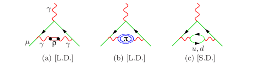
Figure 1: Leading is the hadronic photon vacuum polarization of $O(\alpha^{2})$ . Diagrams a) and b) show possible effective model contributions, VMD and sQED, respectively, and diagram c) the pQCD tail. The safe method of its evaluation is a dispersion relation in conjunction with experimental $e^{+}e^{-}\to\gamma^{*}\to\mathrm{hadrons}$ data or lattice QCD (in progress).

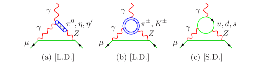
Figure 2: Mixed weak hadronic effects. Again we have low energy effective theory diagrams (L.D.) and the quark-loop diagram (S.D.). Only the VVA vertex beneath the $\pi^{0}Z$ coupling contributes since VVV$\equiv$0. As manifest on the level of the quarks, anomaly cancellation is at work, which implies that potentially large effects $O(\alpha\,G_{\mu}\,m_{\mu}^{2}\ln M^{2}_{Z}/m^{2}_{\mu})$ cancel. Therefore small and well under control.

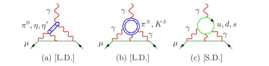
Figure 3: Hadronic light–by–light scattering of $O(\alpha^{3})$ . Diagrams (a) and (b) represent the long distance (L.D.) contributions, diagram (c) involving a quark loop which yields the short distance (S.D.) tail. Internal photon lines are dressed by $\rho-\gamma$ mixing. This is the most challenging part and also suffers from conceptual problems.

Figures 1,2 and 3 illustrate the need for hadronic effective modeling of the dominant long distance (L.D.) piece, while the short distance (S.D.) tail is calculable by perturbative QCD (pQCD) [quark-loops], in principle. The AMM of the muon is a hot topic these days in view of two new muon $g-2$ experiments to come. A muon spinning in a homogeneous magnetic field $\vec{B}$ in absence of an electric field $\vec{E}$ shows a Larmor spin precession frequency $\vec{\omega}$ directly proportional to $\vec{B}$ : $\vec{\omega}_{a}=\frac{e}{m}\,[a_{\mu}\vec{B}]\;.$ The new Fermilab experiment is improving the “magic energy” technique, based on tuning the beam energy to nullify the electric focusing field $\vec{E}$ coefficient $(a_{\mu}-1/(\gamma^{2}-1))=0$ ($\gamma$ the Lorentz factor), and the planned J-PARC experiment attempting to work in a strict $\vec{E}=0$ environment. The first method requires ultra relativistic muons (CERN, BNL, Fermilab)), the second novel concept will work with ultra cold muons (J-PARC) and has very different systematics.

Then the AMM measurement amounts to measuring the Larmor precession frequency of the circulating muons and the magnetic field by the nuclear magnetic resonance method (Larmor precession of protons in a H²O sample) and the present precision is expected to improve by a factor 4. The present mismatch $\Delta a_{\mu}=a_{\mu}^{\mathrm{the}}-a_{\mu}^{\mathrm{exp}}=(-30.6\pm 7.6)\times 10^{-10}$ would increase to a $6\,\sigma$ deficiency of the SM prediction if theory is taken as today and the central value would not move. Improving theory by reducing the hadronic uncertainty by a factor 2 could result in a significance of $11\,\sigma$.

A general introduction I have presented recently in Jegerlehner:2018zrj (see also my recently actualized book Jegerlehner:2017gek ) and the present short note should be considered as a supplement with a focus an the role of meson physics in this game. The hadronic vacuum polarization (HVP) part I have reviewed not long ago in Jegerlehner:2015stw ; Jegerlehner:2017lbd and I will be short on that and focus more on the HLbL part.

2 To be improved: leading hadronic=mesonic effects

The problem is a reliable and precise evaluation of the non-perturbative strong interaction effects. Besides the dispersion relation (DR) approach applicable where the relevant experimental cross sections are available one needs low energy effective hadronic modeling like vector meson dominance (VMD), scalar QED (sQED), extended Nambu-Jona-Lasinio (ENJL) or hidden local symmetry (HLS) or similar Resonance Lagrangian Approach models, which attempt to extend chiral perturbation theory (CHPT) by including vector mesons (VMD) in accord with the chiral structure of QCD. Lattice QCD ab initio calculations come closer in precision and already have provided important constraints and information (see e.g. Meyer:2018til ).

The difficulty of getting precise estimate of the non-perturbative effects I illustrate for the HVP contribution (see Fig. 1) in the following Table 1, with entries from DR, VMD, sQED and perturbative QCD (pQCD) adopting alternatively constituent and current quark masses. Only the VMD yields a reasonable agreement with the data-driven DR method while other estimates widely differ and badly fail. This kinds of problems become even more severe in estimating the HLbL contribution which is a 3 scale problem, while the HVP is a comparatively simple 1 scale problem.

Table 1: Low energy effective estimates of the leading vacuum polarization effects $a^{\rm had}_{\mu}(\mathrm{vap})$. For comparison: $5.8420\times 10^{-8}$ for $\mu$–loop, $5.9041\times 10^{-6}$ for $e$–loop

. data+DR $\rho^{0}$–exchange $\pi^{\pm}$–loop QCD [$u,d$] quark-loops [280,810] MeV BW+PDG sQED constituent quarks current quarks $\mathbf{4.2666\times 10^{-8}}$ $4.2099\times 10^{-8}$ $1.4154\times 10^{-8}$ $2.2511\times 10^{-8}$ $4.4925\times 10^{-6}$

2.1 Leading order HVP

Adopting the data-driven DR approach the leading hadronic contribution HPV from the photon vacuum polarization is dominated by the $e^{+}e^{-}\to\pi^{+}\pi^{-}$ channel to about 75%. The major part is determined by the low lying $\rho,\,\omega$ and $\phi$-resonances and in the 1 to 2 GeV region by exclusive channel data as listed in Table 2. Besides a tiny contribution from nucleon pair production all kinds of mesonic states contribute. These have been measured quite exhaustively by BaBar. Because of the high precision required also small contributions are to be kept under control.

Table 2: Exclusive channels in the range [0.305,1.8] GeV based on locally weighted averaged data, which compares to a similar Table 5.3 of Jegerlehner:2017gek where $\omega$ and $\phi$ are taken as BW resonances using PDG parameters and $\pi\pi$ data from different experiments are combined by taking weighted averages of integrals in overlapping regions. The HLS effective theory allows us to predict the cross sections: $\pi^{+}\pi^{-},\leavevmode\nobreak\ \pi^{0}\gamma,\leavevmode\nobreak\ \eta\gamma,\leavevmode\nobreak\ \eta^{\prime}\gamma,\leavevmode\nobreak\ \pi^{0}\pi^{+}\pi^{-},\leavevmode\nobreak\ K^{+}K^{-},\leavevmode\nobreak\ K^{0}\bar{K}^{0}$ . The HLS missing part $4\pi,5\pi,6\pi,\eta\pi\pi,\omega\pi$ etc., in any case is evaluated using data directly. The CHPT low energy tail and the final state radiation (FSR) channel $\pi^{+}\pi^{-}\gamma$ are added separately. Values in units $10^{-10}$.

final state	contrib.	stat	syst	final state	contrib.	stat	syst
$\pi^{0}\gamma$	5.34	0.78	0.85	$K_{S}K^{\pm}\pi^{\mp}$	0.78	0.11	0.12
$\pi^{+}\pi^{-}$	501.55	73.01	79.58	$K_{S}K_{L}\eta$	0.12	0.02	0.02
$\pi^{+}\pi^{-}\pi^{0}$	49.15	7.15	7.80	$K^{+}K^{-}\eta$	0.00	0.00	0.00
$\eta\gamma$	0.56	0.08	0.09	$K^{+}K^{-}\pi^{+}\pi^{-}$	0.32	0.05	0.05
$\pi^{+}\pi^{-}2\pi^{0}$	17.87	2.60	2.84	$K^{+}K^{-}\pi^{0}\pi^{0}$	0.04	0.01	0.01
$2\pi^{+}2\pi^{-}$	13.54	1.97	2.15	$K_{S}K_{L}\pi^{0}\pi^{0}$	0.11	0.02	0.02
$\pi^{+}\pi^{-}3\pi^{0}$	0.74	0.11	0.12	$K_{S}K_{L}\pi^{+}\pi^{-}$	0.08	0.01	0.01
$2\pi^{+}2\pi^{-}\pi^{0}$	0.98	0.14	0.15	$K_{S}K_{S}\pi^{+}\pi^{-}$	0.01	0.00	0.00
$2\pi^{+}2\pi^{-}\eta$	0.03	0.00	0.00	$K^{+}K^{-}\pi^{+}\pi^{-}\pi^{0}$	0.02	0.00	0.00
$2\pi^{+}2\pi^{-}2\pi^{0}$	0.64	0.09	0.10	$K_{S}K^{\pm}\pi^{\mp}\pi^{0}$	0.12	0.02	0.02
$3\pi^{+}3\pi^{-}$	0.11	0.02	0.02	$\phi\eta$	0.01	0.00	0.00
$\pi^{+}\pi^{-}4\pi^{0}$	0.03	0.00	0.00	$\eta\pi^{+}\pi^{-}\pi^{0}$	0.01	0.00	0.00
$\omega\pi^{0}$	0.83	0.12	0.13	$\omega\eta$	0.02	0.00	0.00
$K^{+}K^{-}$	22.26	3.24	3.53	—————————-
$K^{0}_{S}K^{0}_{L}$	14.13	2.06	2.24	sum no CHPT, no FSR	630.26	91.74	100.00
$\omega\pi^{+}\pi^{-}$	0.01	0.00	0.00	sum	637.12	92.74	100.00
$\eta\pi^{+}\pi^{-}$	0.01	0.00	0.00	sum HLS	599.85	0.50	91.74
$K^{+}K^{-}\pi^{0}$	0.16	0.02	0.03	sum non HLS	37.27	2.51	5.43
$K_{S}K_{L}\pi^{0}$	0.69	0.10	0.11

Narrow resonances I usually include as Breit-Wigner (BW) states using PDG parameters. For the low energy region below $1.05\leavevmode\nobreak\ \mbox{GeV}$ (covering $\rho,\,\omega$ and $\phi$) I obtain $a_{\mu}^{\rm had}[E<1.05\leavevmode\nobreak\ \mbox{GeV}]=505.75_{\rho}(0.83)(2.57)[2.70]+35.23_{\omega}(0.29)(0.69)[0.75]+34.31_{\phi}(0.27)(0.38)[0.47]=575.29(0.92)(2.92)[2.84]$, while using data directly I find $a_{\mu}^{\rm had}[E<1.05\leavevmode\nobreak\ \mbox{GeV}]=577.46_{\rm data}(0.71)(4.02)[4.08]$ in units $10^{-10}$ with statistical, systematic and total errors. This illustrates the fair agreement between different treatments of the data. The total leading order HVP contribution in the first case yields $a_{\mu}^{\rm had}=688.65(1.03)(3.82)[3.96]\times 10^{-10}$ while using local averaging of the $\pi\pi$ data the second yields a slightly higher but less precise $a_{\mu}^{\rm had}=690.82(0.85)(4.85)[4.92]\times 10^{-10}$. The low energy two body channel together with the $3\pi$ one can be subjected to a global HLS fit Benayoun:2012wc which yields 83.4% of the total and as a best fit estimate one finds: $a_{\mu}^{\rm had}=(681.9\pm 3.2)\times 10^{-10}=(569.04[1.08]_{\rm HLS-fit}+112.82[3.01]_{\rm HLS-missing})\times 10^{-10}$. For a comparison with other results see Fig. 6 in Jegerlehner:2018zrj (see also Ananthanarayan:2013zua ; Davier:2017zfy ; Keshavarzi:2018mgv ).

2.2 HLbL

The HLbL contribution is dominated by single particle exchanges. Thereby $e^{+}e^{-}\to e^{+}e^{-}\gamma\gamma^{*}\to e^{+}e^{-}\,\mathrm{\bf hadrons}$ data provide important experimental constraints on hadronic transition form factors (TFF). As indicated one of the photons is quasi real in order to get the required sufficient statistics, while the second is off-shell. Fig. 4-left shows the available data which constrain the $\pi^{0}\gamma\gamma^{*}$ form factor of Fig. 3a and Fig. 4-right the pion-loop amplitude of Fig. 3b. Actually, besides the pseudoscalars also axial-, scalar- and tensor-mesons contribute. An overview of various HLbL one-particle exchange contributions is given in Table 3 (see also JN ; Nyffeler:2017ohp ; Bijnens:2017trn ; Knecht:2018sci ). While the $\pi^{0}$ exchange contribution clearly dominates, it is obvious that the other contributions sum to about one-third of the leading one and have to be determined with comparable precision. This is a highly non-trivial task and has been estimated by a very few groups (HKS HKS95 , BPP BijnensLBL ; Bijnens:2017trn , MV MV03 ) only. The simplest channel is the dominant $\pi^{0}$ one and has been evaluated by many groups in many different models/approaches as listed in Table 5.13 of Jegerlehner:2017gek where also the references are given. The relative stability of the results is not very surprising because the relevant $\pi^{0}\gamma\gamma$ transition form factor is constrained by the known $\pi^{0}\to\gamma\gamma$ decay rate, fixing ${\cal F}_{\pi^{0}\gamma\gamma}(m_{\pi}^{2},0,0)$, and by QCD asymptotic behavior of ${\cal F}_{\pi^{0}\gamma\gamma^{*}}(m_{\pi}^{2},0,-Q^{2})$ when $Q^{2}$ gets large, essentially the Brodsky-Lepage (BL) constraint $\propto 1/Q^{2}$ as supported by experimental data (see Fig. 4-left). A new important constraint

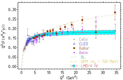
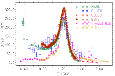
Figure 4: Left: pion production in $\gamma\gamma$ by CELLO, CLEO, BaBar and Belle measurements of the $\pi^{0}$ form factor ${\cal F}_{\pi^{0}\gamma^{*}\gamma}(m_{\pi}^{2},-Q^{2},0)$ at high space–like $Q^{2}$. Towards higher energies BaBar is somewhat conflicting with Belle. The latter conforms with theory expectations, which we use as an OPE constraint. More data are available for $\eta$ and $\eta^{\prime}$ production. Right: di-pion production in $\gamma\gamma$ fusion. At low energy we have direct $\pi^{+}\pi^{-}$ production and by strong rescattering $\pi^{+}\pi^{-}\to\pi^{0}\pi^{0}$, however with very much suppressed rate. With increasing energy, above about 1 GeV, the strong $q\bar{q}$ resonance $f_{2}(1270$ appears produced equally at expected isospin ratio $\sigma(\pi^{0}\pi^{0})/\sigma(\pi^{+}\pi^{-})=\frac{1}{2}$. This demonstrates convincingly that we may safely work with point-like pions below 1 GeV.

has been obtained from lattice QCD by calculating ${\cal F}_{\pi^{0}\gamma^{*}\gamma^{*}}(m_{\pi}^{2},-Q^{2},-Q^{2})$ Gerardin:2016cqj . A first dispersive calculation of the pion-loop contribution $a_{\mu}^{\pi-{\rm box}}+a_{\mu,J=0}^{\pi\pi,\pi-{\rm pole}\,{\rm LHC}}=-24(1)\times 10^{-11}$ has been presented in Colangelo:2015ama . A new solid data-driven evaluation of the pion-pole contribution (in the pion pole approximation) based on the dispersive model yields a fairly precise $a_{\mu}^{{\rm HLbL}\,\pi^{0}}=6.26^{+0.30}_{-0.25}\times 10^{-10}$ Hoferichter:2018kwz . Also a new estimate of the scalar contribution $a_{\mu}^{\rm HLbL-scalars}\simeq(-0.8\pm 7.1)\times 10^{-11}$ has been worked out in Knecht:2018sci . The scalar contribution should be negative in any case. For more details I refer to Jegerlehner:2018zrj or to my book Jegerlehner:2017gek .

Table 3: Estimates of one-particle exchange contributions to HLbL. Leading is the $\pi^{0}$ exchange which amounts to about 65% of the total HLbL. Numbers in units $10^{-11}$.

contribution		individual			total
pseudoscalars	$a_{\mu}^{\mbox{\tiny{LbL}}}(\pi^{0},\eta,\eta^{\prime})$	64.68	14.87	15.90	$95.45\pm 12.40\phantom{2}\phantom{2}$
axials	$a_{\mu}^{\mbox{\tiny{LbL}}}(a_{1},f_{1},f_{1}^{\prime})$	1.89	5.19	0.47	$7.55\pm\phantom{2}2.71\phantom{2}\phantom{2}$
scalars	$a_{\mu}^{\mbox{\tiny{LbL}}}(a_{0},f_{0},f_{0}^{\prime})$	-0.17	-2.96	-2.85	$-5.98\pm\phantom{2}1.20\phantom{2}\phantom{2}$
tensors	$a_{\mu}^{\mbox{\tiny{LbL}}}(f_{2}^{\prime},f_{2},a_{2}^{\prime})$	0.79	0.07	0.24	$1.1\phantom{2}\pm\phantom{2}0.1\phantom{2}\phantom{2}\phantom{2}$
sum single meson exchange					$98.12\pm 12.75\phantom{2}\phantom{2}$
+ $\pi^{\pm},K^{\pm}$ loops + quark loops					$103.40\pm 28.80\phantom{2}\phantom{2}$

My estimate is $a_{\mu}^{\rm HLbL}=[{95.45(12.40)}{+7.55(2.71)}{-5.98(1.20)}{+20(5)}{-20(4)}{+2.3(0.2)}{+1.1(0.1)}{+3(2)}]\times 10^{-11}=103.4(28.8)\times 10^{-11}$. For a comparison with other evaluations see Table 5.19 and Fig. 5.66 of my book Jegerlehner:2017gek . Agreement between different estimates is not yet satisfactory, and a reduction of the errors is still a major issue. Progress we expect from lattice QCD and/or from the dispersive approach (Colangelo et al. Colangelo:2015ama , Pauk and Vanderhaeghen Pauk:2014rta ), which is determining the various HLbL amplitudes based on data and DR’s.

3 Summary and conclusion

The relevance of different mesonic effects in relation to the new experimental result to come are tabulated in Table 4.

Table 4: Significance of typical channels at present and as expected after the new experimental result. In units $10^{-10}$ or in Standard Deviations (SD), present relative to present combined uncertainty $7.6\times 10^{-10}$, coming relative to expected experimental uncertainty $1.6\times 10^{-10}$. The table (bold entries) shows where uncertainties have to be reduced.

type		contribution	SD present	SD coming
HVP	LO $O(\alpha^{2})$	689.5[3.3]	90.7[0.4]	431[2.1]
	$\pi^{+}\pi^{-}$	505.7[2.7]	66.6[0.4]	316.1[1.7]
	$K^{+}K^{-}$	22.0[0.7]	2.9[0.1]	13.8[0.4]
	$\pi^{+}\pi^{-}2\pi^{0}$	20.4[0.9]	2.6[0.1]	12.8[0.6]
	1.05-2GeV	62.2[2.5]	8.2[0.3]	38.9[1.6]
	HO $O(\alpha^{n})$ ($n>2$)	-8.7[0.1]	1.1[0.0]	5.4[0.0]
HEW	3 families	-1.5[0.0]	small by anomaly cancellation
HLbL	all $O(\alpha^{3})$	10.3[2.9]	1.4[0.4]	6.4[1.2]
	$\pi^{0}$	6.3[0.8]	0.9[0.1]	4.1[0.5]

The present status of the SM prediction of $a_{\mu}$ is summarized in Table 5.

Table 5: Standard model theory and experiment comparison [in units $10^{-10}$].

Contribution	Value$\times 10^{10}$		Error$\times 10^{10}$		Reference
QED incl. 4-loops + 5-loops	11 658 471.	886	0.	003	Aoyama12am ; Laporta:2017okg
Hadronic LO vacuum polarization	689.	46	3.	25	Jegerlehner:2017zsb
Hadronic light–by–light	10.	34	2.	88	Jegerlehner:2017gek
Hadronic HO vacuum polarization	-8.	70	0.	06	Jegerlehner:2017zsb
Weak to 2-loops	15.	36	0.	11	Gnendiger:2013pva
Theory	11 659 178.3		4.3		–
Experiment	11 659 209.	1	6.	3	Bennett:2006fi
The. - Exp. 4.0 standard deviations	-30.	6	7.	6	–

What the 4 $\sigma$ deviation is about? Is it new physics? a statistical fluctuation? underestimating uncertainties (experimental, theoretical)? do experiments measure what theoreticians calculate? Is the Bargmann-Michel-Telegdi equation of a Dirac particle in external electromagnetic fields sufficiently accurate? Could real photon radiation affect the measurement?

A “New Physics” interpretation of the persisting 3 to 4 $\sigma$ deviation requires relatively strongly coupled states in the range below about 250 GeV. The problem is that LEP, Tevatron and LHC direct bounds on masses of possible new states $X$ typically say $M_{X}>800\mbox{GeV}$ . In any case $a_{\mu}$ constrains BSM scenarios distinctively and at the same time challenges a better understanding of the SM prediction.

Progress on the theory side requires more/better data and/or progress in non-perturbative QCD. The muon $g-2$ prediction is limited by hadronic uncertainties, which are dominated by meson form factors uncertainties. Substantial progress would be possible if one could reach better agreement on what QCD predicts for the various meson form factors. Most important is the pion sector be it the $\gamma\pi^{+}\pi^{-}$ or the $\gamma\gamma\pi^{0},\gamma\gamma\pi^{+}\pi^{-},\gamma\gamma\pi^{0}\pi^{0}$ and related TFFs. A big challenge for the meson physics community. The most promising dispersive methods require primarily improved data, which is not easy to get.

Fortunately, lattice QCD is making big progress and begins to help to settle hadronic issues. For both of the critical contributions HVP and HLbL lattice QCD will be the answer one day (see Meyer:2018til and references therein), I expect. But a lot remains to be done while a new $a^{\rm exp}_{\mu}$ is on the way!

Acknowledgments
Many thanks to the organizers for the kind invitation to the MESON 2018 Conference and for giving me the opportunity to present this talk and thank you so much for your kind support.

References

- (1) G. W. Bennett et al. [Muon G-2 Collab.], Phys. Rev. D 73 (2006) 072003.
- (2) J. Grange et al. [Muon g-2 Collab.], arXiv:1501.06858 [physics.ins-det]
- (3) T. Mibe [J-PARC g-2 Collab.], Nucl. Phys. Proc. Suppl. 218 (2011) 242
- (4) F. Jegerlehner, Acta Phys. Polon. B 49, 1157 (2018)
- (5) F. Jegerlehner, Springer Tracts Mod. Phys. 274, pp.1 (2017)
- (6) F. Jegerlehner, EPJ Web Conf. 118, 01016 (2016)
- (7) F. Jegerlehner, EPJ Web Conf. 166, 00022 (2018)
- (8) H. B. Meyer, H. Wittig, arXiv:1807.09370 [hep-lat].
- (9) M. Benayoun et al., Eur. Phys. J. C 73, 2453 (2013), Eur. Phys. J. C 75, 613 (2015)
- (10) B. Ananthanarayan et al., Phys. Rev. D 89 (2014) 036007; Phys. Rev. D 93 (2016) 116007
- (11) M. Davier, A. Höcker, B. Malaescu, Z. Zhang, Eur. Phys. J. C 77, 827 (2017)
- (12) A. Keshavarzi, D. Nomura, T. Teubner, Phys. Rev. D 97, 114025 (2018)
- (13) F. Jegerlehner, A. Nyffeler, Phys. Rept. 477, 1 (2009)
- (14) A. Nyffeler, arXiv:1710.09742 [hep-ph].
- (15) J. Bijnens, EPJ Web Conf. 179, 01001 (2018)
- (16) M. Knecht, S. Narison, A. Rabemananjara, D. Rabetiarivony, arXiv:1808.03848 [hep-ph].
- (17) M. Hayakawa, T. Kinoshita, A. I. Sanda, Phys. Rev. Lett. 75, 790 (1995); Phys. Rev. D 54, 3137 (1996); M. Hayakawa, T. Kinoshita, Phys. Rev. D 57, 465 (1998) [Erratum-ibid. D 66, 019902 (2002)];
- (18) J. Bijnens, E. Pallante, J. Prades, Phys. Rev. Lett. 75, 1447 (1995) [Erratum-ibid. 75, 3781 (1995)]; Nucl. Phys. B 474, 379 (1996); [Erratum-ibid. 626, 410 (2002)]
- (19) K. Melnikov, A. Vainshtein, Phys. Rev. D 70, 113006 (2004)
- (20) A. Gérardin, H. B. Meyer, A. Nyffeler, Phys. Rev. D 94, 074507 (2016)
- (21) G. Colangelo, M. Hoferichter, M. Procura, P. Stoffer, JHEP 1509, 074 (2015); Phys. Rev. Lett. 118, 232001 (2017); JHEP 1704, 161 (2017)
- (22) M. Hoferichter, B. L. Hoid, B. Kubis, S. Leupold, S. P. Schneider, arXiv:1808.04823 [hep-ph].
- (23) V. Pauk, M. Vanderhaeghen, Eur. Phys. J. C 74, 3008 (2014)
- (24) T. Aoyama, M. Hayakawa, T. Kinoshita, M. Nio, Phys. Rev. Lett. 109 (2012) 111808
- (25) S. Laporta, Phys. Lett. B 772, 232 (2017)
- (26) F. Jegerlehner, arXiv:1711.06089 [hep-ph].
- (27) C. Gnendiger, D. Stöckinger, H. Stöckinger-Kim, Phys. Rev. D 88 (2013) 053005.