Distances for WiFi Based Topological
Indoor Mapping

Abstract

For localization and mapping of indoor environments through WiFi signals, locations are often represented as likelihoods of the received signal strength indicator. In this work we compare various measures of distance between such likelihoods in combination with different methods for estimation and representation. In particular, we show that among the considered distance measures the Earth Mover’s Distance seems the most beneficial for the localization task. Combined with kernel density estimation we were able to retain the topological structure of rooms in a real-world office scenario.

I Introduction

Indoor localization and mapping through WiFi signals has received a lot of interest in research through the recent years. This interest has largely been accelerated through the prevalent use of smartphones, as these allow for localization without the need of any specialized additional hardware. Since nowadays WiFi access points (APs) are present in most situations within buildings, no additional infrastructure needs to be installed. One typical method for localization and mapping in this realm is to compare the distributions of received signal strength indicators (RSSIs). An advantage of this method is that the APs do not need to be modified. Therefore localization and mapping can be performed virtually everywhere.

A difficult problem that frequently arises in such scenarios is to measure the (dis)similarity between two RSSI distributions. This (dis)similarity then is interpreted as a (dis)similarity of locations in the following way: similar measurements belong to nearby locations. This notion of dissimilarity enables us to apply unsupervised machine learning procedures, e.g., clustering, in order to identify locations. Some techniques were already introduced to measure (dis)similarities between RSSI distributions (e.g., [13]). However, they were often used in supervised machine learning scenarios. The focus there is not necessarily on quality of the applied distance measure, but on learning through labeled examples.

In this paper we investigate various distance measures between sets of WiFi observations, where we also consider various representational methods for the measurements. Since WiFi signals suffer from strong variance even when the location is not changed, we especially consider representations through discrete and continuous probability distributions which allow for modeling the uncertainty in RSSI observations.

In this work we focus on the following scenario. First, pedestrians move indoors with a smartphone following their normal behaviour, e.g., at the work place. Secondly, our aim is to infer sets of locations, i.e., we want to recognize from recorded WiFi signals whether some location is revisited or whether a different location is visited. Thirdly, we do not require that additional infrastructure or software is installed at the locations.

Our contributions are as follows: (1) To the best of our knowledge, this work is the first thorough study of various measures of distance between RSSI distributions. (2) We describe a simple method to group together RSSI measurements which are made at a single location when a smartphones is not moved. (3) We substantiate our study with a real world office scenario experiment over five days. Our participants in this experiment simply follow their normal day behaviour, while carrying a smartphone. This is in contrast to research where participants are instructed to walk along predefined paths or to hold their smartphone in a specific way.

II Problem Statement

We will start by introducing the task and constraints in an informal way. After that we give a formal problem definition and finally, decompose the problem into feasible subproblems.

II-A Task and requirement definition

Our ultimate aim is to compute topological maps from signal strength measurements of WiFi access points (APs). The measurements are made passively through people carrying smartphones while they follow their normal behaviour. A topological map should reflect which physical locations there are and how these locations are related to each other. In this paper, we focus on the recognition and discrimination of distinct physical locations through measured WiFi signal strengths. Physical locations can, for example, be a kitchen where people brew coffee or a canteen where people have lunch. In a more fine-grained scenario, physical locations could refer to the $\varepsilon$-neighborhood of points in a floor plan. In our experiments we will, however, only consider the case where locations are defined on the room level.

We pose the following constraints on a solution for this task:

1. Independent: Our method should work without any need of additional infrastructure at the physical locations to be mapped.

2. Automatic: Our method should not require a specific user behaviour (as for example keeping the smartphone in your hand pointing into the walking direction).

3. Effortless: No user interaction or manual place annotation should be needed.

4. Lightweight: We aim at a lightweight approach, i.e., few data should be needed and, following the notion of Occam’s razor, the model complexity should be low.

In this work we consider a scenario where a set of distinct physical locations should be recognized from a set of WiFi measurements. In addition to that we want to assign these measurements to physical locations in order to perform device localization. This should be achieved without the help of any ground truth, i.e., through an unsupervised method.

To discriminate sets of measurements, one needs, first, a representation of the measurements (often called a fingerprint of a location), and secondly, a measure of dissimilarity or distance between the representations. In supervised localization, RSSI measurements are often represented as vectors where each component denotes the RSSI of a specific access point measured at a point in time [3]. We, however, only consider representations through probability distributions of RSSI values. These distributions will be conditioned on locations. Hence, we call those conditional distributions RSSI likelihoods. The reason for considering RSSI likelihoods is that single RSSI measurements have strong random fluctuations, even when the location is stable. A probability distribution can represent these fluctuations. Additionally, probability distributions naturally allow for further inferences, e.g., localization of previously unseen measurements through maximum likelihood or determining a confidence of being at some location (which is the reason for choosing the name RSSI likelihoods).

We consider several methods to estimate and represent RSSI likelihoods and various measures of distance between them. While some authors consider a distance measure as a synonym for a metric, we consider in this work a more general notion.

Definition 1 (Distance measure on X).

A distance measure on a set $X$ is a function $d:X\times X\rightarrow\mathbb{R}_{\geq 0}$ such that for all $a,b\in X$ we have $a=b\implies d(a,b)=0$.

Nonetheless, we will require that a distance measure gives an interpretation of dissimilarity, where a higher distance is interpretable as higher dissimilarity. Our aim is to find the best combination of likelihood estimation and distance measure, such that calculated distances between RSSI likelihoods reflect real distances between the physical locations appropriately. To evaluate particular combinations we consider first, properties of the distance measure, secondly, discriminative strength, thirdly, correlations with $L_{2}$ distances in a floor plan. The latter two will be evaluated through a real-world experiment.

II-B Formal Problem Definition

Our input data consists of timestamped WiFi observations made by devices, e.g., smartphones, which we identify with a person carrying it. A WiFi observation is the received signal strength indicator (RSSI) measured by a device from an AP. We use RSSI measurements, because of the relation between signal strengths and physical distances to APs. Each AP is uniquely identified through a basic service set identifier (BSSID).

Definition 2 (WiFi data set).

We call the quaternary relation $W\subseteq\mathbb{N}\times D\times B\times R$ WiFi data set, where $\mathbb{N}$ represents timestamps, $D$ is a set of devices, $B$ a set of BSSIDs and $R=[-100,-10]\cap\mathbb{Z}$ a range of RSSI values. A WiFi observation $o\coloneqq(t,d,b,r)\in W$ contains the RSSI value $r$ of WiFi access point $b$ sensed at timestamp $t$ by device $d$. For all $(t,d,b,s_{1}),(t,d,b,s_{2})\in W$ it shall hold that $s_{1}=s_{2}$.

We require $\check{L}\subseteq W\times W$ to be an equivalence relation (i.e., reflexive, symmetric and transitive relation) which reflects the true association between observations and physical locations. So, we suppose the existence of some ground truth for distinct or equal physical locations in the WiFi observations. Hence, this requires that for all $(t,d,b_{1},r_{1})\in W\text{, }(t,d,b_{2},r_{2})\in W$ there holds $((t,d,b_{1},r_{1}),(t,d,b_{2},r_{2}))\in\check{L}$, i.e., a device cannot be at different locations at the same time. Any equivalence relation, like $\check{L}$, gives rise to a partition on the base set, like $W$, and vice versa. We can obtain for $\check{L}$ a partition of $W$ by $\check{\mathcal{P}}=W/L=\{[o]_{\check{L}}\mid o\in W\}$ with the sets $[o]_{\check{L}}=\{o^{\prime}\in W\mid(o,o^{\prime})\in\check{L}\}$ called equivalence classes. Our aim now is to compute a partition $\mathcal{P}$ of $W$ which approximates $\check{\mathcal{P}}$.

Problem 1 (Location Identification).

For a given WiFi data set $W$ with $\check{\mathcal{P}}$, find a partition $\mathcal{P}$ of $W$ such that an error function $E(\mathcal{P},\check{\mathcal{P}})$ is low.

Let $\bar{L}$ be the equivalence relation related to the partition $\mathcal{P}$, i.e., $\bar{L}=\{(o,o^{\prime})\in W\times W\mid\exists P\in\mathcal{P}:\{o,o^{\prime}\}\in P\}$. The elements of $\mathcal{P}$, representable by $[o]_{\bar{L}}$, are called the observed locations, as opposed to the physical locations. Using this we denote by $L_{d,t}\coloneqq[t,d,b,r]_{\bar{L}}\in{W}/{\bar{L}}$ the location of device $d$ at time $t$. The formulation of 1 using partitions reflects our presumed notion of solving location identification problems through clustering. This constitutes our ultimate goal. However, in this work we focus on a simpler variant of this task. By lifting the restriction of computing a partition in favor of computing a family of sets, we may employ other approaches to the location identification problem. This relaxation comes with the price of loosing the strong connection between partitions and equivalence relations. Hence, we fall back to an approximation of the true location relation by some relation $L$ on $W$.

Problem 2 (Location Discrimination).

For a WiFi data set $W$ with $\check{L}$, compute $L\subseteq W\times W$ such that $\hat{E}(L,\check{L})$ is low.

We will approach 2 through a distance measure $d$. For this we suppose we can find for any approximation $L$ some threshold $\tau\in\mathbb{R}_{>0}$ such that for $O,O^{\prime}\subseteq W$ with $O\cap O^{\prime}=\emptyset$ it holds that $d(O,O^{\prime})<\tau\iff\forall(o,o^{\prime})\in O\times O^{\prime}:(o,o^{\prime})\in L$. The goal now is to find $L$ through suitable sets $O\subseteq W$.

II-C Problem Decomposition

Finding out which WiFi observations belong to the same location in a data set is a difficult problem due to sensor differences across devices, measurement noise and signal disturbances through objects, walls and multi-path effects. We will therefore decompose Problem 2 into two easier problems. First, we restrict our investigation to the problem where $|D|=1$. Hence, we restrict the WiFi data set to a particular device d and denote its WiFi data set by $W_{d}\subseteq W$. Secondly, we will exploit detecting the stationarity of a device (i.e., a device not in movement). Hence, observations made during an interval of stationarity can be assigned to one single location. The recognition of such intervals poses an additional problem. Deciding stationarity or movement (possibly changing locations) will be done through acceleration sensor data, since acceleration leads to movement and commonly smartphones possess an acceleration sensor. Acceleration typically is measured along three axes, which can be denoted as a vector. We calculate the norm of the vector, because it is invariant to the rotation of a device, therefore not requiring a specific user behaviour of holding the smartphone.

Definition 3 (Acceleration data set).

An acceleration data set is a relation $A\subset\mathbb{N}\times D\times\mathbb{R}$. We call $(t,d,a)\in A$ an acceleration observation. The value $a$ denotes the Euclidean norm of some acceleration vector $\mathbf{a}=(a_{x},a_{y},a_{z})^{T}\in\mathbb{R}^{3}$ measured by device $d$ at timestamp $t$.

Problem 3 (Motion Mode Segmentation).

For a device $d$ in a WiFi data set, find a segmentation of time $\sigma_{d}=(t_{0},t_{1},...,t_{n})$ such that $d$ is stationary in the interval $[t_{i},t_{i+1})$ if $i$ is even and in movement if $i$ is odd. One such interval is called a segment and two consecutive segments of a device alternate between states of stationarity and movement.

From a motion mode segmentation, we infer that all of the device’s WiFi observations made in a stationary segment belong to the same location. We will use the segmentation to further restrict $W_{d}$ to the data where $d$ is stationary, i.e., to the intervals $[t_{i},t_{i+1})$ from $\sigma_{d}$ where $i$ is even. Our disjoint sets of observations, to which we apply our distance measure, will then be constructed by $W_{d,i}\coloneqq\{(t,d,b,r)\in W_{d}\mid t_{i}\leq t<t_{i+1}\}$ for all even $i\in\mathbb{N}<n$. We will call these sets stationary WiFi segments or simply WiFi segments.

III Method

Figure 1: Visualization of our approach. Blocks indicate processes. Arrows are annotated by in-/outputs.

Our method, as depicted in Figure 1, works as follows: First, we perform motion mode segmentation based on the acceleration data. We then estimate the RSSI likelihood for each stationary WiFi segment. In particular we investigate on various methods to estimate the likelihood based on discrete and continuous probability distributions. To quantify dissimilarities between the likelihoods, we calculate their pairwise distances through a distance measure on probability distributions. We omitted the step location discrimination here, which we will present in Section IV.

III-A Motion Mode Segmentation

Motion mode segmentation is done in a bottom-up-approach consisting of two parts. First, we represent the acceleration data of a device as a time series $\{a_{t}\}_{t\in\mathbb{N}}$ and classify short time intervals as either movement or stationarity. We do this by applying a sliding window to the series, calculating a window function and thresholding it for classification. As a window function, we used the energy [9]. However, utilizing the sample variance gave similar results. We determined a decision threshold through a decision tree. This method achieved about 96% accuracy in a 10-fold crossvalidation on a small activity recognition data set. Secondly, we aggregate consecutive windows from the same class. This gives us the final motion mode segmentation, i.e., an $n$-tuple of the timestamps where modes of movement start and end.

III-B Segment Representation

We assume that the true likelihoods are unique and thus we can recognize and distinguish locations through the dissimilarities between likelihood estimates made from WiFi observations. Formally, we assume there is a conditional probability distribution $p(r_{1},r_{2},...,r_{m}\,|\,L_{d,t})$ for each location $L_{d,t}$ where $r_{k}$ is a random variable for the RSSI measured from access point $b_{k}$. This conditional distribution is the presumed true likelihood of observing a combination of RSSI values given the location. We will also make the assumption that given a location, the signal strenghts of different access points are conditionally independent. Thus, their conditional joint distribution can be factorized.

$$p(r_{1},r_{2},...,r_{m}\,|\,L_{d,t})=\prod_{k=0}^{m}{p(r_{k}\,|\,L_{d,t}})$$ (1)

This assumption has been frequently made for representing RSSI likelihoods in previous research (e.g., in [17]). However, there are some arguments against it. For example, different rotations of the person carrying a device cause signals from varying directions being damped by the body. Clearly, if a different rotation is not considered as a different location, then there is some dependence between signals. Furthermore, we assume implicitly that the distribution is independent of time, while in reality this clearly is not the case. As an example, a change in the environment can change the signal distribution. However, we assume that our approximation in combination with a distance measure is still close enough to rerecognize locations in reasonably short time spans and robust enough for small changes in the environment or rotations of the body.

We consider the WiFi observations made during a stationary segment as samples from the underlying distribution. Thus, for each stationary WiFi segment $W_{d,i}\subseteq W_{d}$ with samples from the interval $[t_{i},t_{i+1})$, we calculate an estimate $\hat{p_{i}}$ of the underlying true likelihood $p_{i}$.

In Equation 1 we assumed that the conditional joint distribution of the RSSI values is a product of the RSSI likelihoods of each single AP. In the following, we will therefore introduce several methods for estimating the factors in (1), i.e., the RSSI likelihoods for single access points.

Representation through a Probability Mass Function

We frst consider estimating the RSSI likelihood of an access point as a discrete probability mass function (PMF). Hence, we model each factor in (1) as a normalized histogram with bin size one, i.e., to each possible RSSI-value we assign the probability mass of its relative frequency. With our WiFi data set this can easily be done through counting the RSSI values, which are given as integers.

Formally, let $W_{d,i}^{k}\coloneqq\{(t,d,b_{k},r)\in W_{d,i}\}$ be a device’s measurements of the signal strengths received from access point $b_{k}$ during the segment $[t_{i},t_{i+1})$. We estimate the probability of receiving a signal strength of $r^{\prime}$ from access point $b_{k}$ given the location $L_{d,t}$ of the segment $[t_{i},t_{i+1})$ as follows:

$$\hat{p_{i}}(r_{k}=r^{\prime}\,|\,L_{d,t})\coloneqq\frac{|\{(t,d,b_{k},r^{\prime})\in W_{d,i}^{k}\}|}{|W_{d,i}^{k}|}$$ (2)

If $|W_{d,i}^{k}|=0$, i.e., no observations are made for $b_{k}$ during the segment, we assign the full probabillity mass of 1 to an RSSI of $-100$. This is slightly lower than the lowest value we observed in any experimental measurements. Thus we model the situation of an invisible access point as observing a very low signal strength. This ensures that we have valid probability distributions for all APs, even when no values were observed. Also this representation is useful for calculating distances. If an AP is visible in one WiFi segment and invisible in another this will increase the distance between their RSSI likelihoods.

Representation through a Normal Distribution

This estimation is based on the assumption that the true RSSI likelihoods are normally distributed. We thus estimate $\hat{p_{i}}$ by

$$\hat{p}_{i}(r_{k}=r^{\prime}\mid L_{d,t})\sim\mathcal{N}(\hat{\mu}_{i},\hat{\sigma}_{i}^{2})$$ (3)

where $\hat{\mu}_{i}$ and $\hat{\sigma}_{d}^{2}$ are the sample mean and sample variance of the RSSI values of one AP in a WiFi segment. Formally, let $R_{d,i}^{k}=\{r^{\prime}\mid(t,d,b_{k},r^{\prime})\in W_{d,i}^{k}\}$ be the RSSI values of AP $b_{k}$ in a WiFi segment. Then we calculate $\hat{\mu}_{i}$ and $\hat{\sigma}_{i}^{2}$ for $b_{k}$ by:

$$\hat{\mu}_{i}=\frac{1}{|R_{d,i}^{k}|}\sum_{r\in R_{d,i}^{k}}{r},\quad\hat{\sigma}_{i}^{2}=\frac{1}{|R_{d,i}^{k}|-1}\sum_{r\in R_{d,i}^{k}}{(r-\hat{\mu}_{i})^{2}}$$ (4)

Representation through Kernel Density Estimation

Kernel density estimation (KDE) is a technique for estimating a continuous probability density function (PDF) from a given set of samples from the underlying distribution. We will explain KDE for the univariate case here. Let $\{x_{1},x_{2},\cdots,x_{n}\}$ be a set of samples from a univariate, continuous random variable $X$. Then the kernel density estimate $\hat{p}$ of the PDF of $X$ is

$$\hat{p}(x)=\frac{1}{nh}\sum_{i=1}^{n}{k\left(\frac{x-x_{i}}{h}\right)},$$ (5)

where $k$ is called a kernel or kernel function and subject to $k(x)\geq 0$ and $\int_{-\infty}^{\infty}{k(x)dx}=1$. The parameter $h\in\mathbb{R}_{>0}$ is the bandwidth of the kernel. A higher bandwith leads to a smoother probability density estimate. In our experiments, we use the Gaussian kernel, which leads to the probability density estimate being a mixture of $n$ Gaussians with standard deviation $h$ and means located at the sample locations $x_{i}$:

$$k(x)\coloneqq\frac{1}{\sqrt{2\pi}}\exp{\left(-\frac{1}{2}x^{2}\right)}$$ (6)

Laplace Smoothing

Some of the considered distance measures, which we will introduce in the next section, cannot handle zero probabilities. As an example, the symmetrized Kullback–Leibler (KL) divergence is undefined when $p(x)$ or $q(x)$ is zero for an outcome of a random variable $x$. The Bhattacharyya distance is undefined when $BC(p,q)=0$, i.e., when the distributions $p$ and $q$ do not overlap. This is because the logarithm of zero is undefined and goes to negative infinity as $x$ goes to $0$. This problem does not occur when RSSI likelihoods are estimated through a normal distribution or through KDE with a Gaussian kernel, since all densities are then strictly positive. However, when a discrete PMF is employed, we apply Laplace smoothing to compensate for this problem, i.e., we add a small constant to each probability and normalize the probabilities such that their sum is one. This procedure is justifiable through Cromwell’s rule [15], which states that one should never assume a zero probabilitiy of an outcome of a random variable, if one cannot be absolutely sure that it will never occur. Certainly, we cannot be absolutely sure that an RSSI value can not occur at a location, just because we did not observe it in our measurements. In fact it is very likely that we will observe some different RSSI values, especially when we estimated the likelihoods from few samples. Zero probabilities also could easily break further inferences, e.g. location estimation through maximum likelihood, since the product of the likelihoods of an observed RSSI vector would become zero, when the likelihood of an RSSI value is zero at a location just for one single AP.

Modelling Probabilities of AP Invisibilities

For a (smartphone) device scanning all WiFi channels in the 2.4 GHz and 5GHz band takes about three seconds in practice. Hence, only one RSSI value per AP can be measured during such a scan. We may therefore obtain sometimes too few samples in cases where (stationary) segments are short. Also, in practice, many of the RSSI values will be overlooked by the (smartphone) device during a scan, i.e., the AP will be invisible to the scanning device. The probability of observing or missing an RSSI value is a distinct feature of a location by itself and therefore provides further useful information for characterizing locations. Approximately, the probability of AP invisibility is decreasing with increasing signal strength of the AP. We model this probability by extending our WiFi data set through pseudo-observations of $-100$ RSSI values for all APs that were not observed at a recorded timestamp. Formally, for every distinct pair of timestamp and device $(t^{\prime},d^{\prime})$ s.t. $\exists(t^{\prime},d^{\prime},b,r)\in W$ and for every AP $b^{\prime}\in B$, if there exists no $(t^{\prime},d^{\prime},b^{\prime},r)\in W$ we add an observation $(t^{\prime},d^{\prime},b^{\prime},-100)$ to $W$. Then we proceed as before to estimate likelihoods, where the probabilitiy of a $-100$ RSSI now models the probability of AP invisibility at a location, even when some RSSI values were observed from it.

Comparison

There are several advantages and disadvantages of the presented likelihood representations, which we would like to point here. An advantage of using both the normal distribution and the kernel density estimation is that similar probabilities are also assigned to values close to the observed RSSI values. Often it can be the case that a specific RSSI value does not occur in a sample by chance. If only relative frequencies are considered, this leads to a zero probability estimate. However, it is often more appropriate to assume that outcomes close to the observed values can occur with similar probability. As an example, take the case where the RSSI values -70 and -68 have been observed several times during a segment but never the value -69.

A disadvantage of representing segments through a continuous PDF is that assumptions have to be made about the distributions. If a certain distribution is fit to the data, one has to make an assumption about what the underlying distribution of the data is. For RSSI likelihoods, the normality assumption has often been made in literature [14]. In experiments related to the presented in section IV we experienced cases where a smartphone lying around at the same position often had regular down peaks for a strong AP. This means the RSSI was nearly constant for longer intervals and would once in a while decrease by approximately 10dBm for short intervals. The resulting distribution of the measurements therefore has two modi and is not normally distributed.

If kernel density estimation is employed, arbitrary distributions can be approximated [6]. However, one has to select a bandwidth parameter, which determines how much probability is assigned to the outcomes close to the observations. Choosing a suitable bandwidth parameter is then a task by itself. Another disadvantage of a continuous PDF is that calculations can become computationally more expensive, since summation becomes integration. To compute the density at some point we need to evaluate the kernel function for every distinct sample, whenever kernel density estimation is used. Therefore KDE has additional computational costs.

III-C Distance Calculation Between Segments

There exists a wide variety of distance measures between probability distributions. We denote the PDF or PMF of a distribution through small letters $p$ and $q$ and the cumulative distribution functions (CDF) through big letters $P$ and $Q$. We then consider the distance measures listed in Table I.

Table I: Distance measures between probability distributions and their properties. Note that the Bhattacharyya coefficient is not a distance but a similarity measure, but is crucial for the definitions of the Hellinger distance and the Bhattacharyya distance. We included KL divergence for a similar reason. By Id. of indiscernibles we denote the property $d(x,y)=0\iff x=y$.

Name	Equation	Id. of Indiscernibles	Symmetry	Triangle Inequality
KL Divergence [13]	$KL(p\parallel q)=\int{p(x)\log\frac{p(x)}{q(x)}\mathrm{d}x}$	Y	N	N
Symmetrized KL Divergence [13]	$D(p,q)=KL(p\parallel q)+KL(q\parallel p)$	Y	Y	N
Jenssen Shannon Divergence [12]	$JSD(p,q)={\frac{1}{2}(KL(p\parallel m)+KL(q\parallel m))}\text{, }m\coloneqq\frac{p+q}{2}$	Y	Y	N
Bhattacharyya Coefficient [5]	$BC(p,q)=\int{\sqrt{p(x)q(x)}\mathrm{d}x}$	-	-	-
Bhattacharyya Distance [4]	$D_{B}(p,q)=-\ln\left(BC(p,q)\right)$	Y	Y	N
Hellinger Distance [4]	$H(p,q)={\sqrt{1-BC(p,q)}}$	Y	Y	Y
Kolmogorov-Smirnov Distance [4]	$D(p,q)=\sup_{x}|P(x)-Q(x)|$	Y	Y	Y
Earth Mover’s Distance [11]	$EMD(P,Q)=\int{|P(x)-Q(x)|\mathrm{d}x}$	Y	Y	Y
Absolute Difference of Means	$D(p,q)=\left|\mathbb{E}_{p}[x]-\mathbb{E}_{q}[x]\right|,\ \mathbb{E}_{p}[x]=\int{p(x)x\,\mathrm{d}x}$	N	Y	Y

Since our full joint distributions are high-dimensional (i.e., multivariate), computations for many of these distance measures become intractable due to the increasing computational complexity of the quadrature. Others, e.g., the Kolmogorov-Smirnov distance (which is actually a test statistic), cannot easily be extended to the multivariate case. Therefore we calculate distances between the univariate RSSI likelihoods of single APs and take the sum over all APs (i.e., also those that are invisible). Since all distances are positive, this is the same as calculating the $L_{1}$-norm. In case of the KL divergence it can be shown that if the univariate distributions are independent, this sum is the KL divergence of the joint distributions [13]. To our knowledge the same does not hold for the other distance measures with exception of the symmetrized KL divergence. However, we think that it is reasonable to increase the total distance proportionally with every AP distance. For comparison we also calculate the $L_{2}$-norm, which in turn puts more weight on larger distances. Our distance measure between two multivariate signal strength distributions $p$ and $q$ is therefore defined as

$$d_{\ell}(p,q)=\Big{(}\sum_{k=1}^{m}{d(p(r_{k}),q(r_{k}))^{\ell}}\Big{)}^{1/\ell},\quad\ell\in\{1,2\},$$ (7)

where $p(r_{k})$ and $q(r_{k})$ are the univariate signal strength distributions of AP $b_{k}$ and $d$ is a distance measure from Table I.

At this point we would like to note that, if the used distance measure between single APs is a bounded metric, then also our distance measure $d_{\ell}$ is a metric. Also note that APs invisible in both segments, i.e., both compared distributions, can be omitted to compute Equation 7. This follows from Definition 1.

Considering the distance measures in Table I, we would like to point out that calculating the absolute difference between the expected values is not a metric on probability distributions, since different distributions can have the same mean. Nonetheless, it is a metric on the expected values. Taking the absolute difference of means makes our distance measure equivalent to computing the Manhattan or Euclidean distance between the average RSSI vectors of two segments.

Other work [13] suggests using the symmetrized KL divergence for supervised localization through kernel regression. However, this measure has two disadvantages for the comparison of RSSI likelihoods: First of all, it is not a metric, because the triangle inequality is not required. Distances between physical locations, viewed as points in $\mathbb{R}^{3}$, follow the triangle inequality. Therefore using a metric to compare location representations is more consistent with our view of the physical world. Secondly, consider the case where two distributions do not overlap and there is a gap between them. Then symmetrized KL divergence reaches its maximum value no matter how large the gap is. However, it makes no difference how large the gap between the distributions is. The Earth Mover’s Distance (EMD, [11]) on the other hand becomes larger, the larger the gap between the distributions is. In the case of RSSI likelihoods, it makes sense to infer that locations are farther away from each other when the gap between RSSI likelihoods becomes larger.

IV Experiments

To test our method, we conducted an experiment at our group located in Kassel, Germany. We collected data for five days during work time. Each participant was instructed to carry a smartphone with her as well as an RFID badge clipped to the chest [8]. We recorded WiFi and acceleration data on each smartphone using the Sensor Data Collection Framework [2] (SDCF) for the Android operating system. The RFIDs were used to collect ground truth data. For this we installed stationary RFIDs at several physical locations we considered important. These locations are the desks of participants, which were located in different rooms, our coffee kitchen and a table soccer. The idea here is that whenever two persons meet we can register a contact using the RFID badges. This encounter would be recorded and sent to our servers. The same is true for an encounter of a person with the afore mentioned desks, kitchen or tables soccer. More technically, a contact occurs, when two RFIDs are within a distance of approximately 1.5 meters. Since human bodies block the signal, a contact only occurs when a person’s chest points roughly towards another RFID. Participants were additionally instructed to fill in manual logs about their locations and activities, which can be used for plausibility tests. In total, eight people took part in the experiment. To ensure device heterogenity, we used several different smartphone models, as depicted in Table II. One of the participants carried two smartphones.

Table II: Experiment participants and used smartphones.

PersonID	Device Model	5GHz	Data used
1	Samsung GT-I9195	Y	N
2	LG Nexus 4	Y	Y
3	LG Nexus 5	Y	Y
3	HTC One X+	Y	Y
4	OnePlus 5	Y	N
5	HTC One X+	Y	Y
6	Jiayu S3+	Y	N
7	Samsung GT-I9001	N	N

Some smartphone models could not reliably record data over longer periods of time. Some minutes after starting the data collection process through the SDCF the collection process was unintentionally stopped. We suspect this problem occurs due to vendor specific battery saving measures integrated into the operating system. For other participants, we could not collect much data because they were mostly not present at our group during the experiment or the batteries of their devices did not last long enough. In total, we used the data from four devices for our experiments. Altogether, we collected about 1.38 Million WiFi observations adding up to roughly 247 hours. The data from the four smartphones used in the evaluation adds up to about 40 hours on average per device.

IV-A WiFi Data Preprocessing

In some cases, RSSIs from mobile APs, e.g., hotspots raised by mobile phones themselves, are observed. Since these APs are likely to change their location, we ignore observations from them, i.e., remove them from the WiFi data set. These APs are often recognizable through their Service Set Identifier (SSID), i.e., the name of the WiFi network. Examples of such APs are Tim’s iPhone, AndroidHotspot or Porsche. Due to a parking lot next to our building, many of such car hotspots appeared in our recordings. We remove mobile APs through a manually crafted blacklist of SSID-prefixes and postfixes. However, we observed that the relative amount of such recordings was comparably low. Hence, we think their negative influence on localization is not very strong and often mitigated through other APs, even if some mobile hotspots are overlooked. As a final preprocessing step, we only include stationary WiFi segments with a minimum duration of ten seconds in our analysis. This is because we think that shorter durations contain too few samples to estimate RSSI likelihoods.

IV-B Ground Truth Preprocessing

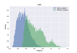
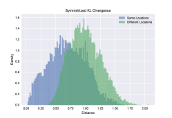
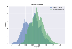
Figure 2: Normalized histograms of calculated distances for LG Nexus 4. In each plot, the left histogram depicts distances between segments from the same location, the right histograms distances between different locations. Likelihoods were estimated through PMF and invisible APs included.

Ground truth data from RFIDs is sparse. As addressed before, a person’s spatial orientation can lead to a (human) body blocking the RFID signal. Additionally, objects interfering with the 2.4GHz or 5GHz band do block or damp signals. We therefore enhance our ground truth in two ways: First, we make use of the symmetry of contacts. If an RFID badge $a$ receives a contact signal sent from an RFID badge $b$, we enhance our data by adding a pseudo contact signal received by $b$ from $a$. Secondly, we aggregate contacts, which were initially recorded at distinct timestamps, to time intervals. We assume that for two fixed badges, if the timestamp difference between two contacts is lower than a given threshold, then there has been a contact for the whole interval duration. As a threshold we use the difference of one minute. We chose this value based on the comparison of RFID data to the manual logs of the participants. However, there is a trade-off between correctness and availability of ground truth. While a too big interval threshold can introduce errors to the ground truth, a too small one leads to sparser data.

IV-C Discriminative Evaluation

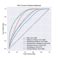
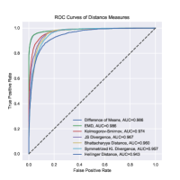
Figure 3: ROC Curves: HTC One X+ (left), Nexus 5 (right). For all distance measures, likelihoods were estimated as PMF and AP invisibilities included.

One aim of using a distance measure on RSSI likelihoods is to find out whether two sets of observations were made at the same physical location. This task can be treated as a binary classification problem. Based on this we developed the following evaluation scheme. We represent each set of observations made at one day in one room as a signal strength distribution as introduced in Section III-B. Using this we then calculate the distances between all possible pairs of signal distributions from the same room and from different rooms. Figure 2 shows histograms of the calculated distance values. The left histogram there in each plot contains the distances calculated between the same room. The histograms to the right there in each plot depict distances calculated between different rooms. The lower the overlap between the histograms, the more capable our distance measure is of discriminating rooms.

Let us now consider a binary classifier which discriminates the same from different locations by thresholding (see Section II-B) on the distance measure Equation 7.

$$f:P\times P\rightarrow\{0,1\}\text{, }f(\hat{p}_{i},\hat{p}_{j})=\Theta(d(\hat{p}_{i},\hat{p}_{j})-\tau)$$ (8)

In this equation $\Theta$ is the Heaviside step function which returns zero if its argument is smaller than zero, and one otherwise. The value $\tau$ is a threshold. Hence, our classifier returns one if the distance between the two input likelihoods is not smaller than $\tau$. Semantically one is interpreted as the likelihoods stemming from different locations. On different levels of $\tau$, we calculate the true positive rate by $tpr\coloneqq tp/(tp+fn)$ and false positive rate by $fpr\coloneqq fp/(fp+tn)$ of this classification function on our WiFi data set. In this $tp$ and $fp$ denote the number of true positives and false positives, and $tn$ and $fn$ the number of true negatives and false negatives. We then calculate the area under the ROC curve (AUC) to evaluate our distance measure. AUC can be interpreted as the probability of ranking a random positive sample higher than a random negative sample [10]. In our case this is the probability of assigning a higher distance to a random pair of segments from different locations than to a pair of segments from the same location. An example of the resulting ROC curves and AUC values is given in Figure 3.

IV-D Evaluation of Correlations

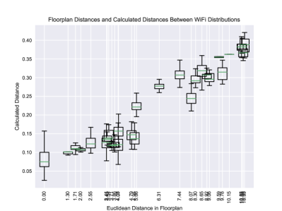
Figure 4: Correlations between floor plan distances and calculated distances between RSSI likelihoods for one device. Left: Several distances are calculated for the same pairs of true locations, hence distributions of the calculated distances are given through box plots. Right: We present the mean calculated distance for the y-coordinate. Euclidean distance between distribution means were applied. Correlations: Pearson 0.94, Kendall: 0.79, Spearman; 0.92.

To evaluate how well the considered distance measures capture distances between physical locations, we proceed as follows: For the ground truth locations, we determine the position of tags in a floor plan and measure their pairwise distances. We calculate the Pearson correlation coefficient, Spearman’s rank correlation coefficient and Kendall’s tau between calculated and floor plan distances. The Pearson correlation coefficient measures the degree of linear relationship between two variables. Our ratio is that a perfect distance measure would provide perfect linear correlation with floor plan distances. Spearman’s rank correlation coefficient measures the monotonic relationship between variables. In our case this means how well the ranking of the calculated distances matches the ranking of the floor plan distances. Kendall’s tau is a different way to calculate the rank correlation and thus expresses a similar measure as the Spearman rank correlation. Our example in Figure 4 shows a result from our experiment where these correlations are captured for a particular distance measure. In this case a strong correlation can be observed.

IV-E Visual Evaluation

We use multidimensional scaling (MDS) to layout WiFi segments in $\mathbb{R}^{2}$. This method receives a pairwise distance matrix as input and determines coordinates in $\mathbb{R}^{n}$ for a given $n$ such that the distances are preserved optimally. Our ratio here is that the result retains at least topological relations between locations, i.e., segments from the same location should be kept close together. We show an exemplary result of this procedure in Figure 5, where we use the Manhattan distance between expected values. The results for other participants are similar.

Figure 5: Plot of the calculated MDS coordinates for one smartphone. Each point represents a WiFi segment. The segments have been clustered through the HDBSCAN algorithm [7] and colored according to their cluster. Points are annotated by RFID contacts, which give hints about true locations.

The results indicate, that indeed topological structures are retained through our method. We recognize six main clusters, not of all which are annotated through ground truth data. The ground truth is as follows: 0-desk, 5-desk in neighbored room, 3-table soccer, 2-kitchen, 1-desk near the kitchen and 4-table directly next to the kitchen. The other three clusters could be identified from our manual logs as a bathroom, the canteen and a food store located next to our building. For the annotated locations, topological relations were mostly retained, i.e., the bureau labeled by 0 is indeed halfway in between the other two locations. However this does not hold for the relations between the three unlabeled locations. These locations are very far away from each other and do not have any APs in common. There are specific areas, where locations are hardly distinguishable through WiFi signals alone. We attribute this to little AP coverage and thin walls, since we also found these difficulties in our related supervised localization experiments.

IV-F Discussion

We calculated ROC curves and correlations for the four used smartphones and all distance measures in all kinds of combinations of modelling likelihoods and including AP invisibilities in the distributions or not. In total, we consider seven distance measures, each with $L_{1}$ norm and $L_{2}$ norm. We have three ways of modelling distributions and two possibilities for counting invisible APs or not counting them. Altogether we have $84$ combinations of calculating distances for each smartphone and therefore $336\cdot 4$ performance measures to compare. Due to limited space we may only sum up our main findings. The full evaluation results as well as our WiFi data set are available from our web page (https://kde.cs.uni-kassel.de/datasets).

In the results we observed in general, that measures with better AUC implied better correlations with floorplan distances. Similarly, when one correlation was stronger, the other correlations were stronger. We addressed this partially in Section IV-D.

IV-F1 Distance Measures

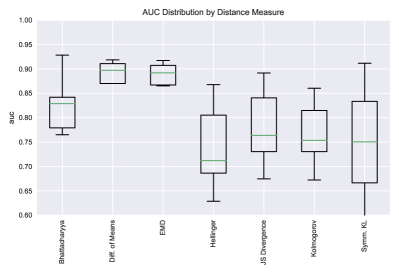
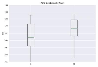
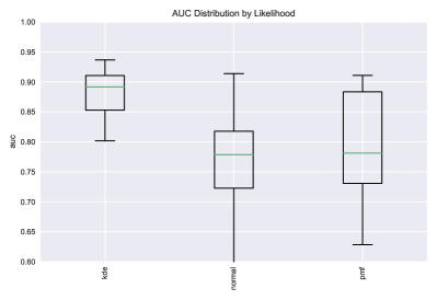
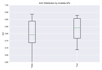
Figure 6: Distribution of calculated AUC values for various groups.

Figure 6 shows summary statistics of the calculated AUC values for various distance measures. A surprising result to us is that simple absolute distances between expected values of the distributions often gave the best performance. Our actual intuition was that a measure, which does not consider the subtle differences between distributions, could not capture these distances well. Therefore, our actual intention was to include this measure as a baseline.

Another surprising result was that EMD often gave almost the same results as the absolute distance between the means and therefore performed about equally well. This seems obvious to us and can be explained as follows: Consider two univariate CDFs. For EMD, we calculate the area between both curves. Now consider the case where each CDF jumps from $0$ to $1$ in a small interval where the measured RSSI-values are located. Let the positions of these intervals be located far away from each other. Then the area between both curves is approximately proportionate to the distance between those small intervals. Therefore, EMD is often dominated by the absolute difference of the mean RSSI values. We expected EMD to perform well because of its properties, e.g., it fulfills the triangle inequality. Therefore, it coincides with our intuition that there cannot be any shortcut to the direct path between two locations over a third location. It also incorporates the distance between non-overlapping distributions and provides smoothing through the CDF. Therefore it was no surprise to us, that the calculated distances are stable across different likelihood estimations, which however can also be attributed to the mentioned relation to the absolute difference of means. An advantage of this measure is that it already gives good results with a likelihood representation obtained through a simple counting of RSSI values. We think an advantage of EMD over the absolute differences between means is that it can also capture subtle differences between close distributions, e.g., when their means are similar but their variances or kurtoses differ. For more distant distributions it gives very similar results to the distances between means, which seems a positive property.

Concerning the other distance measures, we sometimes observed specific settings, where similar or even slightly better results could be achieved for some smartphones. However, these measures are a lot more sensitive to the likelihood estimation and the used norm function. We think that stability, and therefore reliability of the used measure, should be preferred.

IV-F2 Euclidean Norm vs. Manhattan Norm

Almost all distance measures profited from calculating the $L_{2}$ norm instead of the $L_{1}$ norm of the distance vector. In particular, ROC curves of worse performing distance measures improved. Although, well performing measures improved only slightly, or did perform weaker. We believe that through the Euclidean norm our distance measure becomes more sensitive to individual greater distances between the univariate distributions. Those distance measures that are bounded by a maximum value, i.e., the distributions do not overlap, and do not differentiate between larger or smaller gaps between the distributions, therefore profit from the $L_{2}$ norm. Nonetheless, we found evidence in literature that for clustering high-dimensional data the $L_{1}$-norm has advantages [1]. However, this does not seem to hold for our data. The reason for this may be found in the fact that we basically compute distances in lower-dimensional sub spaces.

IV-F3 Likelihood Estimation

From the estimation techniques, KDE consistently worked better than using a PMF. We attribute this to the smoother distributions obtained. Therefore they are more robust to the effects of random sampling. Normal distributions gave the lowest performance in our experiments. From a theoretical point of view, it makes little sense to estimate a normal distribution, when AP invisibility should be modeled. This is because such distributions would need to be multimodal.

IV-F4 Modelling AP Invisibility

Representing AP invisibility in the distributions gave strong improvements in most cases, especially in combination with KDE. In [13], localization is achieved only through modelling the multinomials of AP visibilities. We think that representing both, AP invisibilities and RSSI values, is a strong method for location discrimination.

V Summary and Conclusions

In this work we studied various distance measures and representations of WiFi observations. After our investigation we are able to provide the following rules of thumb as recommendations for measuring dissimilarities between RSSI likelihoods. As it turned, applying kernel density estimation for the likelihoods is the method of choice. Also, one should include AP invisibility into the modeling. Finally, the Earth Mover’s Distance can deliver subtle differences for close distributions as well as stable differences for far distributions.

We also unraveled several limitation of our approach. Since all of our observations were measured on the same floor of the building, the results may not be transferable to three dimensional scenarios. However, we believe that the effect of floors and ceilings between vertically stacked rooms is similar as the effect of walls between neighbored rooms. This should be verified in future work. The employed approach for motion mode segmentation may fail whenever artificial acceleration patterns appear, e.g., using an elevator. Nonetheless, utilizing a more elaborate activity recognition system (e.g., [16]) would be able to improve this situation.

Concluding we would like to point out, that our ultimate goal is beyond a localization through distances alone. We rather consider our investigation of distance measures as a building block for more complex localization techniques. Hence, we investigated in this work the properties of this building block. These techniques may not necessarily depend on WiFi. While we were aiming in this work at clustering WiFi distributions, we are convinced our results can be transferred to other scenarios. For example, they may be also applicable in localization scenarios employing Bluetooth low energy (BLE) beacons.

References

- [1] Charu C. Aggarwal, Alexander Hinneburg, and Daniel A. Keim. On the surprising behavior of distance metrics in high dimensional space. In Lecture Notes in Computer Science, pages 420–434. Springer, 2001.
- [2] Martin Atzmueller and Katy Hilgenberg. Towards capturing social interactions with sdcf: An extensible framework for mobile sensing and ubiquitous data collection. In Proceedings of the 4th International Workshop on Modeling Social Media, MSM ’13, pages 6:1–6:4, New York, NY, USA, 2013. ACM.
- [3] P. Bahl and V. N. Padmanabhan. Radar: An in-building rf-based user location and tracking system. In IEEE INFOCOM 2000, volume 2, Tel-Aviv, Israel, March 2000. IEEE.
- [4] Michèle Basseville. Distance measures for signal processing and pattern recognition. Signal Processing, 18(4):349–369, December 1989.
- [5] A. Bhattacharyya. On a measure of divergence between two multinomial populations. Sankhya: The Indian Journal of Statistics, 7(4):401–406, Juli 1946.
- [6] C. M. Bishop. Pattern Recognition in Machine Learning. Springer, 2006. page 123.
- [7] Ricardo J. G. B. Campello, Davoud Moulavi, and Jörg Sander. Density-based clustering based on hierarchical density estimates. In Jian Pei, Vincent S. Tseng, Longbing Cao, Hiroshi Motoda, and Guandong Xu, editors, PAKDD (2), volume 7819 of Lecture Notes in Computer Science, pages 160–172. Springer, 2013.
- [8] Ciro Cattuto, Wouter Van den Broeck, Alain Barrat, Vittoria Colizza, Jean-François Pinton, and Alessandro Vespignani. Dynamics of person-to-person interactions from distributed rfid sensor networks. PloS one, 5(7):e11596, 2010.
- [9] Mostafa Elhoushi, Jacques Georgy, Aboelmagd Noureldin, and Michael J. Korenberg. A survey on approaches of motion mode recognition using sensors. IEEE Trans. Intelligent Transportation Systems, 18(7):1662–1686, 2017.
- [10] J A Hanley and B J McNeil. The meaning and use of the area under a receiver operating characteristic (roc) curve. Radiology, 143(1):29–36, April 1982.
- [11] E. Levina and P. Bickel. The Earth Mover’s distance is the Mallows distance: some insights from statistics. In IEEE ICCV, volume 2, pages 251–256, 2001.
- [12] J. Lin. Divergence measures based on the shannon entropy. IEEE Transactions on Information Theory, 37(1):145 – 151, 1991.
- [13] Piotr W. Mirowski, Harald Steck, Philip Whiting, Ravishankar Palaniappan, Michael MacDonald, and Tin Kam Ho. Kl-divergence kernel regression for non-gaussian fingerprint based localization. In IPIN, pages 1–10. IEEE, 2011.
- [14] Piotr W. Mirowski, Philip Whiting, Harald Steck, Ravishankar Palaniappan, Michael MacDonald, Detlef Hartmann, and Tin Kam Ho. Probability kernel regression for wifi localisation. J. Location Based Services, 6(2):81–100, 2012.
- [15] Giovanni Parmigiani, Lurdes Y T Inoue, and Hedibert F. Lopes. Decision Theory: Principles and Approaches. Wiley Blackwell, 12 2010. page 22.
- [16] He Wang, Souvik Sen, Ahmed Elgohary, Moustafa Farid, Moustafa Youssef, and Romit Roy Choudhury. No need to war-drive: unsupervised indoor localization. In Nigel Davies, Srinivasan Seshan, and Lin Zhong, editors, MobiSys, pages 197–210. ACM, 2012.
- [17] Moustafa Youssef and Ashok Agrawala. The horus wlan location determination system. In MobiSys ’05: Proceedings of the 3rd international conference on Mobile systems, applications, and services, pages 205–218, New York, NY, USA, 2005. ACM.