TESS in the Solar System

Abstract

The Transiting Exoplanet Survey Satellite (TESS), launched successfully on 18th of April, 2018, will observe nearly the full sky and will provide time-series imaging data in $\sim$27-day-long campaigns. TESS is equipped with 4 cameras; each has a field-of-view of $24\times 24$ degrees. During the first two years of the primary mission, one of these cameras, Camera #1, is going to observe fields centered at an ecliptic latitude of $18$ degrees. While the ecliptic plane itself is not covered during the primary mission, the characteristic scale height of the main asteroid belt and Kuiper belt implies that a significant amount of small solar system bodies will cross the field-of-view of this camera. Based on the comparison of the expected amount of information of TESS and Kepler/K2, we can compute the cumulative étendues of the two optical setups. This comparison results in roughly comparable optical étendues, however the net étendue is significantly larger in the case of TESS since all of the imaging data provided by the 30-minute cadence frames are downlinked rather than the pre-selected stamps of Kepler/K2. In addition, many principles of the data acquisition and optical setup are clearly different, including the level of confusing background sources, full-frame integration and cadence, the field-of-view centroid with respect to the apparent position of the Sun, as well as the differences in the duration of the campaigns. As one would expect, TESS will yield time-series photometry and hence rotational properties for only brighter objects, but in terms of spatial and phase space coverage, this sample will be more homogeneous and more complete. Here we review the main analogues and differences between the Kepler/K2 mission and the TESS mission, focusing on scientific implications and possible yields related to our Solar System.

1. Introduction

The Transiting Exoplanet Survey Satellite (TESS) mission is an ongoing full-sky survey initiative, aiming to discover hundreds of rocky planets around main-sequence and dwarf stars (Ricker et al., 2015). TESS orbits Earth in a special high inclination, high eccentricity orbit which has a period commensurable to the sidereal orbital period of the Moon, with a $2:1$ mean motion resonance. Onboard TESS, there are four wide-field cameras, each having $24\times 24$ degree of field-of-view (FOV) while the focal plane array is formed by $4$ frame-transfer CCDs with total dimensions of $2048\times 2048$ pixels. Hence, the pixel scale of TESS is $\sim 21^{\prime\prime}$, however, due to the fast, $f/1.5$ focal ratio, this pixel scale varies slightly throughout the field-of-view. The cameras are aligned in a way that the gross FOV of TESS forms a nearly $96\times 24$ degrees wide strip in the sky.

Observations provided by TESS yield two main types of scientific data: one type of data are in the form of so-called stamps, i.e. sub-frames with a 2-min cadence around several thousands of pre-selected F, G, K and M-type of stars. Another type of data are the full-frame images (FFI), which are provided with a cadence of 30 minutes. During its two-year primary mission, TESS will observe $2\times 13$ fields, called sectors, where its Camera #4 points towards the ecliptic poles and Camera #1 points close to the ecliptic plane, and the alignment of the cameras are parallel with ecliptic longitude great circles (see Fig. 7 in Ricker et al., 2015). There are $13$ partially overlapping sectors defined in the Northern Ecliptic Hemisphere and $13$, also partially overlapping sectors defined in the Southern Ecliptic Hemisphere (see also Fig. 7 in Ricker et al., 2015). Although this primary mission design avoids the ecliptic plane within a distance of $\sim 6^{\circ}$, the characteristic scale height of both the main asteroid belt and the Kuiper belt is significantly larger than this value – namely, the meidan deviation and standard deviation of the inclinations are $\sim 7.1^{\circ}$ and $\sim 11.1^{\circ}$ for the main belt while $\sim 9.8^{\circ}$ and $\sim 24.0^{\circ}$ for the Kuiper belt, respectively, based on the MPCORB.dat.gz file (see Sec. 3). Therefore one can expect that a considerable number of moving objects will be detected by the TESS cameras. Indeed, even a simple query to an up-to-date minor planet database shows that a huge fraction of such bodies will be presented in the TESS FOV(s), mainly in Camera #1 (and a few in Camera #2), see also Fig. 1.

Our goal here is to provide an initial estimate on the TESS yield of photometric data related to minor Solar System bodies. The analysis presented here makes a detailed comparison with the same type of yield of the K2 mission (Howell et al., 2014), which turned out to be a very effective instrument for targeted observations of these minor bodies (Szabó et al., 2015; Pál et al., 2015a). The scientific highlights of the K2 mission include observations of a variety of Kuiper belt objects (Pál et al., 2015a, 2016a; Benecchi et al., 2018), natural satellites of gas giants (Kiss et al., 2016; Farkas-Takács et al., 2017), implications for the detection of the satellite of 2007 OR₁₀ (Kiss et al., 2017), observations of main belt objects crossing K2 superstamps (Szabó et al., 2016; Molnár et al., 2018) and observations of Jupiter Trojans (Szabó et al., 2017; Ryan, Sharkey & Woodward, 2017). Extended and uninterrupted photometric coverage was found to be crucial to unambiguously identify long rotation periods that are commensurable with or longer than the day-night cycle of the Earth. Current asteroid rotation statistics have been found to be biased towards shorter periods by multiple studies (Masiero et al., 2009; Marciniak et al., 2018; Molnár et al., 2018).

The structure of this paper goes as follows. First, in Sec. 2 we briefly summarize the similarities and differences between the TESS and Kepler/K2 missions concerning solar system target observations. In Sec. 3 we describe the set of tools which are used in the TESS yield simulations in terms of observations of small bodies in our Solar System. In Sec. 4, a set of examples are displayed by simulating 30-minute TESS FFI data using the up-to-date catalogues provided by the Minor Planet Center and the Gaia DR2 catalogue (Gaia Collaboration et al., 2016, 2018) for background stars. These simulations focus on both the photometry of known objects, in order to retrieve rotation characteristics, as well as on the estimates of flux excess during the photometry of stars. In Sec. 5, statistics are presented for the expected flux excess of target stars caused by minor planet encounters. We summarize our results and conclude in Sec. 6.

2. Similarities and differences between TESS and Kepler/K2

After the failure of the second reaction wheel of the Kepler Space Telescope (Borucki et al., 2010), the K2 mission was initiated by targeting Kepler to the ecliptic plane in order to minimize the required thruster firing corrections (Howell et al., 2014). These comparatively frequent thruster firing corrections are necessary due to the torques induced by solar radiation pressure and introduces a larger amount of systematic noise in the raw light curves. Similar to the Kepler space telescope, TESS is also designed for extremely precise photometry of stars with fixed positions in the sky. In the following, we list the main similarities and differences of the Kepler/K2 and TESS data acquisition schemes, which will also affect the selection of the most suitable targets within our Solar System.

First, while the typical apparent speed of a main-belt asteroid is $3-5$ pixels per $30$-min long cadence for K2 (Szabó et al., 2016; Molnár et al., 2018), it is significantly smaller in the case of TESS, i.e., it is smaller or close to 1 pixel/cadence ($\lesssim 21^{\prime\prime}/{\rm 30\,mins}$, see also Fig. 2). Therefore, we can make reliable estimates for TESS just considering non-moving targets at first glance – see, e.g., Fig. 14 in Sullivan et al. (2015) or Fig. 8 in Ricker et al. (2015).

Second, in the case of TESS, 30–50% of the objects that cross the field-of-view can be seen throughout the whole one-month campaign. This can easily be computed from the previously mentioned estimates of $\lesssim 1\,{\rm pixel}/{\rm cadence}$ for the apparent speed, the total number of FFI cadences acquired during the observations of a single sector (which is around $\sim 1300$ for a 27-day-long campaign per sector) and the width of the sectors (i.e., the size of the sectors parallel with the ecliptic latitude circles) which is in the range of $4000$ pixels in total. A series of 5 images displaying this behavior is presented in Fig. 3.

In addition, in the case of TESS, minor planets are observed during opposition while K2 observes these closer to their stationary points. Therefore the apparent movement of the objects are correlated, all retrograde, and the velocity dispersion is much smaller than for K2 (see also Figs. 2 and 3).

In order to further quantify our expectations about the usefulness of TESS for solar system science, we ran simulations by involving some of our tools. The main concepts of these simulations and the tools employed therein are described in the following section (Sec. 3) while the resulting light curves are displayed and detailed in Sec. 4.

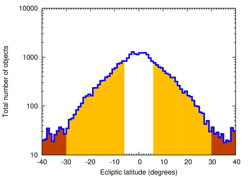
Figure 1.— The number density of the catalogued minor planets in a stripe having a width of 24 degrees as a function of the ecliptic latitude. The orange and brown filled parts correspond to TESS cameras #4 and #3, respectively. The empty part between $\pm 6$ degrees is not observed during the primary mission of TESS.

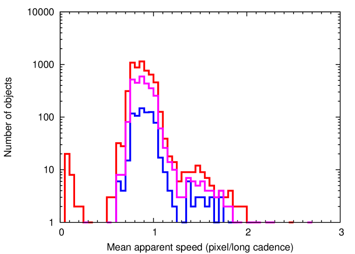
Figure 2.— The number density of the minor planets (Camera #1, closest to the ecliptic plane) as a function of the apparent speed. The red curve shows this number density for all of the catalogued objects, while the purple and blue curves correspond to the objects brighter than $V=20$ and $V=18.5$ magnitudes, respectively. The minor planets have been queried for a single TESS campaign.

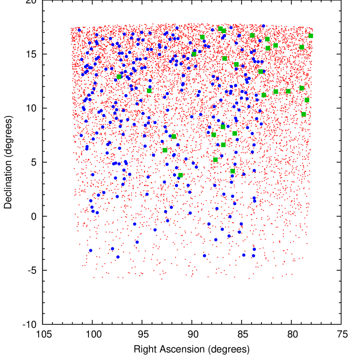
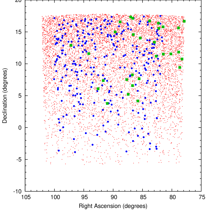
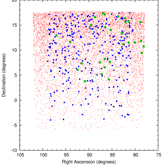
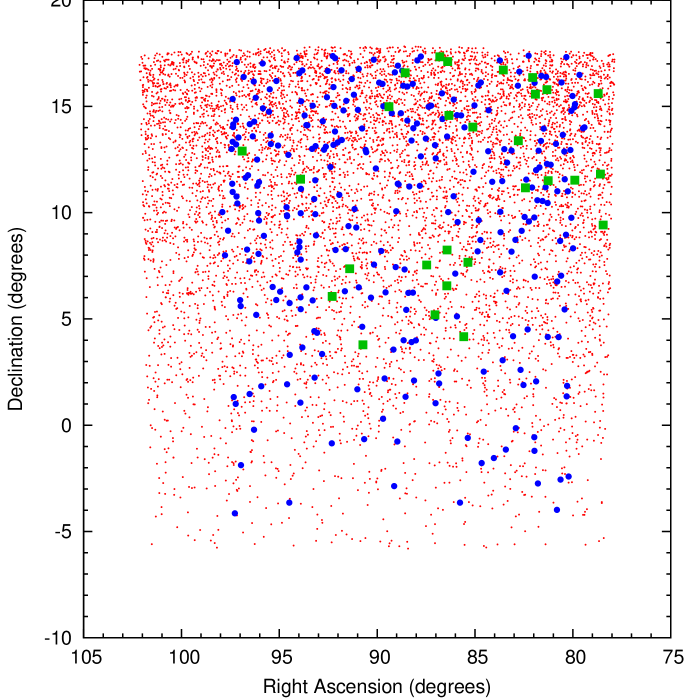
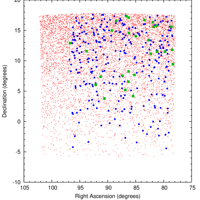
Figure 3.— The series of images above shows all catalogued minor planets (as of 2017 June 12) as it is seen by Camera #1, which is the closest to the ecliptic plane. The cadence between these images are 5 days while the ephemerides of the central image correspond to JD 2458474 (2018 December 21, 12:00 UTC). The small red dots correspond to the catalogued minor planets. For visualization purposes, the blue dots mark every 20th object that can be seen during the whole campaign. In addition, green squares show the positions of trans-Neptunian objects (TNOs). The swarm of the blue dots clearly show that during a one-month TESS campaign effectively all minor planets have a correlated and retrograde motion. Note that only those small bodies that appear in the first panel are displayed throughout the series of figures.

3. Tools for data reduction, analysis and astrometric predictions

In order to get an estimate on the precision and accuracy of Solar System observations, we carried out a series of simulations in a Monte-Carlo fashion. Namely, artificial images were generated which have similar characteristics to TESS, considering both the optical and imaging properties as well as the detector parameters such as readout and other types of noise. This series of simulations was build on the top of four databases and software packages as follows:

• MPCORB.dat.gz – the MPCORB.dat.gz file provided by the Minor Planet Center. This is a simple textual file with several hundreds of thousands of lines, containing orbital elements and brightness parameters (absolute magnitudes and slope parameters) for all of the catalogued minor planets in the Solar System. This file is regulary updated and can be retrieved from the Minor Planet Center. Although online tools (such as MPC itself and JPL/Horizons) exist that can retrieve a series of ephemerides for single or multiple objects, our simulations require the nearly simultaneous handling of all of the available orbital data of minor planets. Therefore, it is easier and safer to handle all of the related computations in an offline fashion since both the number of epochs and the size of the field-of-view(s) are much larger than the intended use-cases of these available online tools.

• Gaia DR2 – the recently published Gaia DR2 catalogue. This catalogue (Gaia Collaboration et al., 2016, 2018) contains records for $\sim 1.6$ billion point sources. Since the wide-band TESS throughput (see Fig. 1 in Ricker et al., 2015) quite well agrees with the Gaia $G_{\mathrm{RP}}$ band (see Fig. 3 in Jordi et al., 2010), this database is rather suitable to simulate the stellar background of the simulated images by employing the $G_{\mathrm{RP}}$ magnitudes (i.e. the 61st, the phot_rp_mean_mag record in the *.csv.gz files in the ./gdr2/gaia_source/csv directory, see also the original database descriptions).

• EPHEMD. While several tools exist which can be used as ephemeris services, none of them are optimized for retrieving a list of Solar System objects that traverse the large field-of-view of TESS. This feature of a service is generally referred as cone search. The web-based service of the Minor Planet Center is suitable only for ground-based observatories while the Virtual Observatory service SkyBoT (Berthier et al., 2016) is capable of identifying minor planets only for a single time instance. While developed mainly for the observations related to the K2 mission (Molnár et al., 2018), here we list some of the features of the tool named EPHEMD, optimized for searches spanning longer time intervals – hence, this tool is also optimal for TESS.

  • EPHEMD is implemented in a server-client architecture. The program itself is running in the background while it caches all of the necessary pre-computed orbits. Simple commands referring to queries and ephemeris services can then be executed while connecting via TCP/IP.

  • The input database of EPHEMD is derived from the file MPCORB.dat.gz. updated by the Minor Planet Center.

  • EPHEMD supports easy integration of various observers (including the Kepler spacecraft and TESS) by involving either SPICE kernels or ephemerides for the observers.

  • The precision of the computations performed by EPHEMD is in the range of $\lesssim 0.02^{\prime\prime}$ with respect to the JPL/Horizons service (namely, differences can only be seen in the last significant digit when one queries positions for 5 decimal places in degrees).

  A more detailed description of this EPHEMD package will be available soon along with the uploading of its source code to the public domain as a free and open source program.

• FITSH. The FITSH package (Pál, 2012) is used as the core of a state-of-the-art pipeline developed for the photometry of Solar System objects in the fields of Kepler/K2 missions (Pál et al., 2015a; Szabó et al., 2016). Features that are relevant for analyzing this type of data include the elongated apertures supported by FITSH/fiphot. In addition, the tasks of FITSH perform astrometric analysis and automated cross-matching of sources, including the computations corresponding to the large optical distortions of the TESS cameras. While this feature is not essential during the simulations, analysis of real data needs such an algorithm, similarly to the way it is employed in the case of K2 superstamps (see, for instance Farkas-Takács et al., 2017; Molnár et al., 2018).

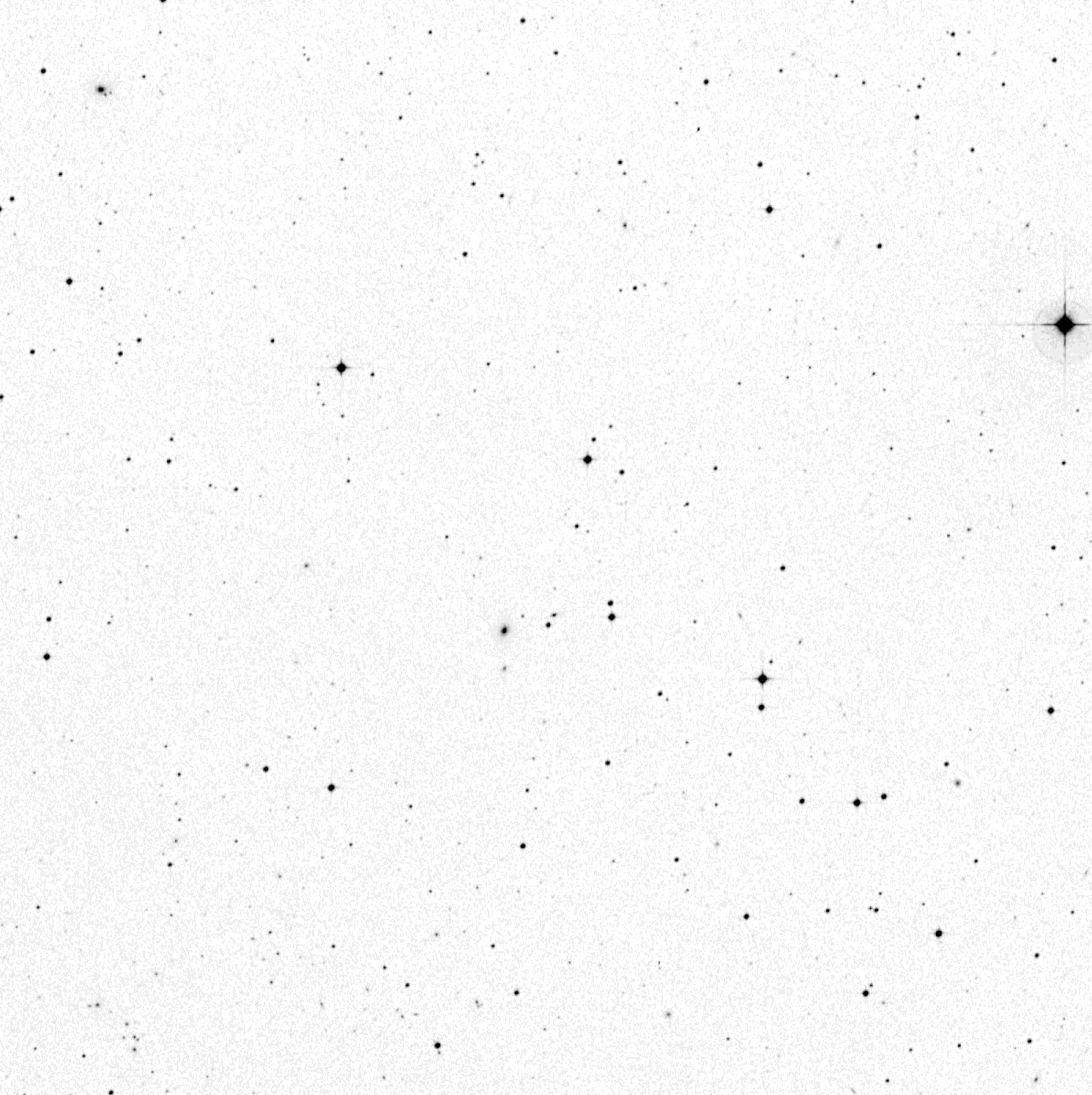
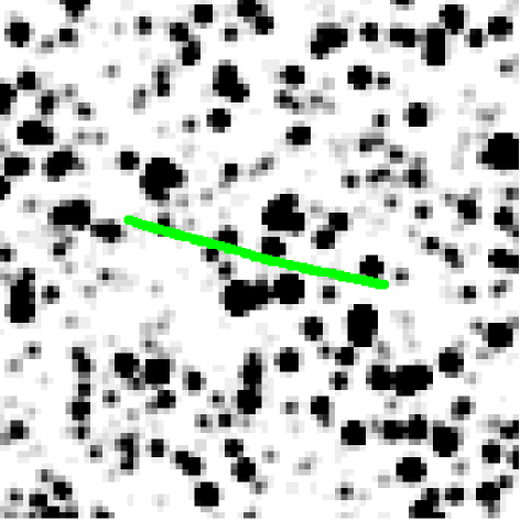
Figure 4.— Simulations of the TESS observations for the dwarf planet Eris. Upper left: The $30^{\prime}\times 30^{\prime}$ field-of-view of the sky, centered at $\alpha=25.842$ and $\delta=-2.262$. This position corresponds to the apparent location of Eris on October 20, 2018. During the first year of science operations, TESS will observe the Southern Hemisphere where Eris is presently located. Upper right: The same field-of-view in the simulated TESS images. During this simulation, the alignment of TESS cameras is set w.r.t. the equatorial reference system. The green line shows the path of Eris as it traverses this field for 27 days. Lower left: Reconstructed folded light curve of Eris, expecting a single-peaked solution with a rotation period of $15.77\,{\rm d}$. The peak-to-peak amplitude of this injected signal is $0.05$ mags. Lower right: Residual spectrum of Eris’ light curve as a function of the rotation frequency. Due to the single-peaked nature, this spectrum is dominated by the peak corresponding to the injected rotation frequency.

The actual simulations are carried out as follows. By retrieving the list of Gaia DR2 sources as well as pre-computed ephemerides of minor bodies, an artificial image is created by the FITSH/firandom tool after applying the appropriate astrometric projections (which convert J2000 ICRS RA and DEC coordinates into the $x,y$ plane of the CCD detector). Shot noise and background noise is added in accordance with the expected signal-to-noise levels (see Fig. 8 in Ricker et al., 2015).

High galactic lat.: $|\beta|\approx 45^{\circ}$        Medium galactic lat.: $|\beta|\approx 20^{\circ}$     Low galactic lat.: $|\beta|\approx 10^{\circ}$

Figure 5.— Simulated light curves of real asteroids having fictitious rotational characteristics for various apparent brightness values and galactic latitudes. These $3\times 4$ panels show light curves with double-peaked harmonic variations, having a period of $P=0.30792\,{\rm d}$ and a peak-to-peak amplitude of $0.3^{\rm m}$. The light curves are continuous and cover a time interval of $20^{\rm d}$, slightly shorter than an observing cycle of a TESS sector. The four rows correspond to mean ${\rm V}$ brightness of $16^{\rm m}$, $17^{\rm m}$, $18^{\rm m}$ and $19^{\rm m}$ while the three columns correspond to galactic latitudes of $|\beta|\approx 45^{\circ}$, $|\beta|\approx 20^{\circ}$ and $|\beta|\approx 10^{\circ}$, respectively. These simulations reveal the effect of the different stellar background densities.

We should note here that due to the nature of this type of analysis, it is not essential to fully incorporate all of the properties of the TESS system. Namely, here we ignored the spatial variations of the point-spread function (which was taken into account in the reference simulations, see Sullivan et al., 2015) and used a simple Gaussian PSF model having a full width at half maximum (FWHM) corresponding to the respective ensquared energy (see Table 1 in Ricker et al., 2015). In addition, the large-scale optical distortions were also neglected. This is mainly due to the fact that signal-to-noise ratios of (fainter) minor planets will predominantly be determined by the confusion of background stars – and this is a much more local effect than the large-scale optical distortions of the TESS optics. The light curves are generated using differential photometry where subtracted images were derived using the corresponding FITSH tools (fiarith, ficonv). If the spacecraft pointing jitter is negligible, simple per-pixel arithmetics are sufficient while in the case of large jitter (even when it contains non-white noise components), image convolution is the most efficient way to retrieve the differential images and use the convolution kernels themselves to optimize the aperture (see Eqs. 80-83 in Pál, 2009). The reference image for differential photometry has been chosen as the median for the given time series.

In the next section, we use these tools to simulate both the light curves of minor planets from artificial TESS images as well as the effects of minor planet encounters on the photometry of target stars. Statistics and expectations about the occurrence rates of such minor planet encounters are presented in the following section.

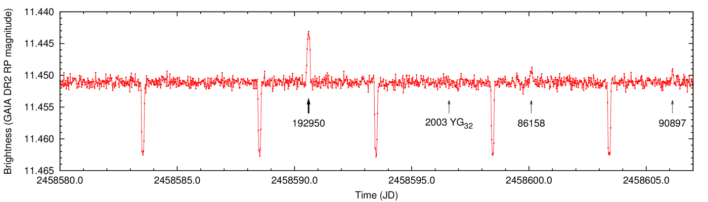
Figure 6.— Simulation of the light curve of the transiting exoplanet host star WASP-83 between JDs 2458580 and 2458607 (Apr 6.5, 2019 and May 3.5, 2019, respectively), in accordance with the expected scheduling of the primary TESS mission. During this period, the target star is encountered by four minor planets where (192950) 2000 BQ₂ is the one with the highest expected brightness of $\sim 16.7^{\rm m}$ in the TESS passbands (assuming a grey color). The encounter with (192950) 2000 BQ₂ would yield an excess in the total brightness around $\sim 8$ millimagnitudes, comparable with the transit depth. In addition, the apparent encounters with (86158) 1999 RY₂₀₃ and (90897) 1997 CF₆ will also yield excesses around $\sim 2$ mmag where the actual objects have an apparent magnitude of $\sim 18.1^{\rm m}$ in the TESS passbands. The faintest one, 2003 YG₃₂ with an apparent brightness of $\sim 21^{\rm m}$ yields no significant excess.

4. Light curve simulations

4.1. (136199) Eris as a target dwarf planet

(136199) Eris is a bright dwarf planet, the most distant known natural object in the Solar System. Recent studies (Sicardy et al., 2011; Santos-Sanz et al., 2012) revealed in an unambiguous manner that its surface is extremely reflective and up to now, no solid rotation period has been estimated for this planet. Since Eris currently has an ecliptic latitude of $\beta\approx-12^{\circ}$, it cannot be observed in the K2 mission but it will be an ideal target for TESS Camera #1. The expected brightness of (136199) Eris is around $\sim 18.1^{\rm m}$ in the TESS passbands. By performing the procedures presented in Sec. 3, we generated a 27-days long light curve of Eris, starting from JD 2458411 and ending at JD 2458438. Like any of the small Solar System bodies, Eris has a retrograde motion during this period while the total span of the object throughout such a TESS campaign of 27 days is approximately $15^{\prime}$. Therefore, one can expect that Eris is a point-like source since this aforementioned motion is equivalent to $\sim 0.03$ TESS pixels per long cadence.

In order to test the expectations of TESS photometric yield, we injected a sinusoidal single-peaked variation in the brightness of Eris, having a peak-to-peak amplitude of $0.05^{\rm m}$ and a period corresponding to the known orbital period of its moon, Dysnomia (15.77 d, Brown & Schaller, 2007). In Fig. 4 we demonstrate that the rotation period with this amplitude can safely be recovered in the frequency space, and the folded light curve is also prominent.

4.2. Main-belt asteroids as target bodies

In order to have an insight about the expected photometric quality of main-belt minor planets, we carried out a series of simulations by implanting variations in the light curves of known bodies. We selected three regions in the sky with higher, intermediate and low galactic latitudes of $|\beta|\approx 45^{\circ}$, $|\beta|\approx 20^{\circ}$ and $|\beta|\approx 10^{\circ}$ and queried for $4+4+4$ objects having a mean visual brightness of $\sim 16^{\rm m}$, $\sim 17^{\rm m}$, $\sim 18^{\rm m}$ and $\sim 19^{\rm m}$. The implanted variations were generated with a periodicity of $P=0.30792\,{\rm days}$ and with a peak-to-peak amplitude of $0.3^{\rm m}$. Here this period of $P=0.30792\,{\rm d}=7.39\,{\rm h}$ corresponds to the median rotation period of the main-belt asteroids as found in Warner, Harris & Pravec (2009). The signal itself was assumed to be a slightly asymmetric double-peaked harmonic function for all cases. The resulting $3\times 4=12$ light curves are displayed on Fig. 5. Note that the mean brightness in the TESS/Gaia ($G_{\rm RP}$) passbands are higher by $\approx 0.7^{\rm m}$ due to the intrinsic color of the Sun. As it can be seen, using these $\sim 20\,{\rm d}$ long signals, the light curve shape can be reconstructed for all of the cases and the effect of the increasing stellar background is also prominent as we go for lower and lower galactic latitudes.

4.3. WASP-83 as a target star

In this section, we present a simulated light curve of WASP-83, an $G_{\rm RP}=11.45^{\rm m}$, late G-type star orbited by a $\sim 1\,R_{\rm Jup}$ planet (Hellier et al., 2015). According to the expected schedule of TESS, this planet host star will be observed around the second half of April 2019.

Due to the low ecliptic latitude, $\beta\approx-13.7^{\circ}$, this star has a quite high chance of nearby encounters by small, foreground Solar System bodies (see e.g. Fig. 1, the expected density of minor planets is around 40% of the peak density). Throughout our simulations, we expected that the corresponding TESS sector is going to be observed between April 6 and May 3, 2019. By exploiting EPHEMD (see Sec. 3 above), we found that within this period, four minor planets would encounter within 0.02 degrees, i.e. within $\lesssim 3$ TESS pixels where one of the objects has a brightness of $\sim$ 1% of the target star. Indeed, the simulated light curve displayed in Fig. 6 clearly features flux excesses during intervals of several hours caused by objects brighter than $19^{\rm m}$.

5. Encounter statistics

In the previous section (Sec. 4.3) we demonstrated a case where the light curve of a known target star harboring a transiting exoplanet is affected by some minor planet encounters. In the following we present brief statistics about the expected number for such encounters, depending on the ecliptic latitudes. In this experiment, we created $36\times 7$ sub-fields, each having a diameter of $1$ degree and distributed uniformly on a grid with a spacing of $10^{\circ}$ along the ecliptic between $\beta=-30^{\circ}$ and $\beta=+30^{\circ}$. For each field, we retrieved the Gaia DR2 catalogue down to $17^{\rm m}$ in the $G_{\mathrm{RP}}$ magnitude and computed the properties of minor planet encounters (within 2 TESS pixels). These encounters were queried during a fictitious TESS sector observation run, lasting for $27$ days and centered at the corresponding anti-Sun longitude at the mid-time of the campaign.

We found that the average number of encounters per star do not depend significantly on the ecliptic latitude, namely for $\beta=\pm 30^{\circ}$, the number of such events is $0.84\pm 0.18$, for $\beta=\pm 20^{\circ}$, it is $1.52\pm 0.22$, for $\beta=\pm 10^{\circ}$ it is $3.67\pm 0.58$ and for the ecliptic itself it is $6.93\pm 0.64$. Considering only the encounters which would yield at least 1% flux increment (i.e., comparable to the transit depth caused by a hot Jupiter), the numbers are somewhat less, i.e. $0.70\pm 0.16$, $1.31\pm 0.17$, $3.07\pm 0.43$ and $5.84\pm 0.47$, for $\beta=\pm 30^{\circ}$, $\pm 20^{\circ}$, $\pm 10^{\circ}$ and $0^{\circ}$, respectively. If we are interested in stars which are brighter than $13^{\rm m}$ in the TESS passbands, then the number of encounters yielding at least 1% flux increment is around $\sim 0.10$, $\sim 0.20$, $\sim 0.39$ and $\sim 0.62$ for $\beta=\pm 30^{\circ}$, $\pm 20^{\circ}$, $\pm 10^{\circ}$ and $0^{\circ}$, respectively. All in all, we conclude by comparing the aforementioned numbers with the the light curve of WASP-83 (see Fig. 6) and knowing that this star has an ecliptic latitude of $\beta\approx-13.7^{\circ}$, that this star can be considered as a rather “typical case” regarding the expected effects of minor planet encounters on the light curve.

6. Summary

Similar to the Kepler/K2 mission, Solar System objects can be considered either as targets of observations or noise and/or flux excess sources for stars. We found that in each campaign, rather good photometry can be achieved for some thousands of minor planets. Light curves are uninterrupted for several dozens of rotations and basic physical characteristics can be derived for objects with very long rotational periods as well – without any ambiguity. While most of the trans-Neptunian objects are too faint for TESS, the brighter ones can also be targets of interest. Most notably, the dwarf planet Eris will also fall on silicon during the primary mission. Eris is bright enough for TESS photometry and moves on a field which is not significantly confused by stars. We also found that minor planets affect the photometric aperture for several hours due to the lower spatial resolution. Here we note that these tools of ours can also be applied to wide-field ground-based surveys, including full-sky monitoring such as in the KELT (Pepper et al., 2007), Fly’s Eye (Pál et al., 2013, 2016b), Evryscope (Law et al., 2015) or MASCARA (Snellen et al., 2012) initiatives.

We emphasize that extended mission setups of the TESS spacecraft can have versatile pointing configurations where the vicinity of the ecliptic can be covered more effectively – i.e., filling the gap at $|\beta|\lesssim 6^{\circ}$, between the northern and southern primary survey areas and/or filling the gaps between the prime mission sectors at $6^{\circ}\lesssim|\beta|\lesssim 30^{\circ}$, see also Bouma et al. (2017). Such configurations will yield not only important follow-up observations for the K2 mission but also much more possibilities for Solar System studies. Other proposals, however, argue for increasing the time coverage and/or the size of the continuous viewing zone at the expense of the total spatial coverage (see e.g. the “Camera 3 on the ecliptic pole”, C3PO configuration of Huang et al., 2018). These setups yield field-of-view only at higher ecliptic latitudes (e.g. $30^{\circ}\lesssim|\beta|$ for C3PO or $42^{\circ}\lesssim|\beta|$ when the spacecraft reference pointing is set to the ecliptic poles), resulting in significantly lesser number of observations for Solar System objects.

References

- Benecchi et al. (2018) Benecchi, S. D.; Lisse, C. M.; Ryan, E. L.; Binzel, R. P.; Schwamb, M. E.; Young, L. A. & Verbiscer, A. J., 2018, Icarus, 314, 265
- Berthier et al. (2016) Berthier, J.;Carry, B.; Vachier, F.; Eggl, S. & Santerne, A. 2016, MNRAS, 438, 3394
- Borucki et al. (2010) Borucki, W. J., Koch, D., Basri, G., et al. 2010, Science, 327, 977
- Bouma et al. (2017) Bouma, L. G.; Winn, J. N.; Kosiarek, J. & McCullough, P. R. Planet Detection Simulations for Several Possible TESS Extended Missions,
- Brown & Schaller (2007) Brown, M.E. & Schaller, E. 2007, Science, 316, 1585
- Farkas-Takács et al. (2017) Farkas-Takács, A.; Kiss, Cs.; Pál, A.; Molnár, L.; Szabó, Gy. M.; Hanyecz, O.; Sárneczky, K.; Szabó, R.; Marton, G.; Mommert, M.; Szakáts, R.; Müller, T.; Kiss, L. L. 2017, AJ, 154, 119
- Gaia Collaboration et al. (2016) Gaia Collaboration: T. Prusti et al., 2016, A&A, 595, A1
- Gaia Collaboration et al. (2018) Gaia Collaboration; Brown, A. G. A.; Vallenari, A.; Prusti, T.; de Bruijne, J. H. J.; Babusiaux, C.; Bailer-Jones, C. A. L., 2018, Accepted for A&A Special Issue on Gaia DR2 (arXiv:1804.09365)
- Hellier et al. (2015) Hellier, C. et al. 2015, AJ, 150, 18
- Howell et al. (2014) Howell, S. B., Sobeck, C., Haas, M., et al. 2014, PASP, 126, 398
- Huang et al. (2018) Huang, C. X.; Shporer, A.; Dragomir, D.; Fausnaugh, M.; Levine, A. M.; Morgan, E. H.; Nguyen, T.; Ricker, G. R.; Wall, M.; Woods, D. F. & Vanderspek, R. K. 2018, AJ, revised after submission (arXiv:1807.11129)
- Jordi et al. (2010) Jordi, C.; Gebran, M.; Carrasco, J. M.; de Bruijne, J.; Voss, H.; Fabricius, C.; Knude, J.; Vallenari, A.; Kohley, R.; Mora, A, 2010, A&A, 523, A48
- Kiss et al. (2016) Kiss, Cs.; Pál, A.; Farkas-Takács, A. I.; Szabó, G. M.; Szabó, R.; Kiss, L. L.; Molnár, L.; Sárneczky, K.; Müller, T. G.; Mommert, M. & Stansberry, J; 2016, MNRAS, 457, 2908
- Kiss et al. (2017) Kiss, Cs.; Marton, G.; Farkas-Takács, A.; Stansberry, J.; Müller, Th.; Vinkó, J.; Balog, Z.; Ortiz, J.-L.; Pál, A., 2017, ApJL, 838, 1
- Law et al. (2015) Law, N. M. et al., 2015, PASP, 127, 234
- Marciniak et al. (2018) Marciniak, A., et al., 2018, A&A, 610, A7
- Masiero et al. (2009) Masiero, J., Jedicke, R., Ďurech, J., Gwyn, S., Denneau, L., Larsen, J., 2009, Icarus, 204, 145
- Molnár et al. (2018) Molnár, L.; Pál, A.; Sárneczky, K.; Szabó, R.; Vinkó, J.; Szabó, Gy. M.; Kiss, Cs.; Hanyecz, O.; Marton, G.; Kiss, L. L., 2018, ApJS, 234, 37
- Pál (2012) Pál, A. 2012, MNRAS, 421, 1825
- Pál (2009) Pál, A. 2009, PhD Thesis (Eötvös Loránd University)
- Pál et al. (2013) Pál, A. et al. 2013, Astron. Nachtr., 334, 932
- Pál et al. (2015a) Pál, A.; Szabó, R.; Szabó, Gy. M.; Kiss, L. L.; Molnár, L.; Sárneczky, K. & Kiss, Cs. 2015a, ApJL, 804, 45
- Pál et al. (2016a) Pál, A.; Kiss, Cs.; Müller, Th. G.; Molnár, L.; Szabó, R.; Szabó, Gy. M.; Sárneczky, K.; Kiss, L. L., 2016, AJ, 151, 117
- Pál et al. (2016b) Pál, A.; Mészáros, L.; Jaskó, A.; Mező, Gy.; Csépány, G.; Vida, K. & Oláh, K. 2016b, PASP, Vol. 128, pp. 045002.
- Pepper et al. (2007) Pepper, J. et al. 2007, PASP, 119, 923
- Ricker et al. (2015) Ricker, G. R. et al. 2015, J. Astron. Telesc. Instrum. Syst. Vol. 1, id. 014003
- Ryan, Sharkey & Woodward (2017) Ryan, E. L.; Sharkey, B. N. L. & Woodward, Ch. E., 2017, AJ, 153, 116
- Santos-Sanz et al. (2012) Santos-Sanz, P. et al. 2012, A&A, 541, A92
- Sicardy et al. (2011) Sicardy, B. et al. 2011, Nature, 478, 493
- Snellen et al. (2012) Snellen, I. A. G. et al. 2012, Ground-based and Airborne Telescopes IV. Proceedings of the SPIE, Volume 8444, article id. 84440I, 7 pp.
- Sullivan et al. (2015) Sullivan, P. W.; Winn, J. N.; Berta-Thompson, Z. K.; Charbonneau, D.; Deming, D.; Dressing, C. D.; Latham, D. W.; Levine, A. M.; McCullough, P. R.; Morton, T.; Ricker, G. R.; Vanderspek, R. & Woods, D. 2015, ApJ, 809, 77
- Szabó et al. (2017) Szabó, Gy. M.; Pál, A.; Kiss, Cs.; Kiss, L. L.; Molnár, L.; Hanyecz, O.; Plachy, E.; Sárneczky, K.; Szabó, R., 2017, A&A, 599, A44
- Szabó et al. (2016) Szabó, R.; Pál, A.; Sárneczky, K.; Szabó, Gy. M.; Molnár, L.; Kiss, L. L.; Hanyecz, O.; Plachy, E.; Kiss, Cs. 2016, A&A, 596, A40
- Szabó et al. (2015) Szabó, R., Sárneczky, K., Szabó, Gy. M., et al. 2015, AJ, 149, 112
- Warner, Harris & Pravec (2009) Warner, B. D.; Harris, A. W. & Pravec, P. 2009, Icarus, 202, 134