Improving Subseasonal Forecasting in the Western U.S. with Machine Learning

Abstract.

Water managers in the western United States (U.S.) rely on longterm forecasts of temperature and precipitation to prepare for droughts and other wet weather extremes. To improve the accuracy of these longterm forecasts, the U.S. Bureau of Reclamation and the National Oceanic and Atmospheric Administration (NOAA) launched the Subseasonal Climate Forecast Rodeo, a year-long real-time forecasting challenge in which participants aimed to skillfully predict temperature and precipitation in the western U.S. two to four weeks and four to six weeks in advance. Here we present and evaluate our machine learning approach to the Rodeo and release our SubseasonalRodeo dataset, collected to train and evaluate our forecasting system.

Our system is an ensemble of two nonlinear regression models. The first integrates the diverse collection of meteorological measurements and dynamic model forecasts in the SubseasonalRodeo dataset and prunes irrelevant predictors using a customized multitask feature selection procedure. The second uses only historical measurements of the target variable (temperature or precipitation) and introduces multitask nearest neighbor features into a weighted local linear regression. Each model alone is significantly more accurate than the debiased operational U.S. Climate Forecasting System (CFSv2), and our ensemble skill exceeds that of the top Rodeo competitor for each target variable and forecast horizon. Moreover, over 2011-2018, an ensemble of our regression models and debiased CFSv2 improves debiased CFSv2 skill by 40-50% for temperature and 129-169% for precipitation. We hope that both our dataset and our methods will help to advance the state of the art in subseasonal forecasting.

kdd,arxiv kdd,arxiv oldarxiv

1. Introduction

Water and fire managers in the western United States (U.S.) rely on subseasonal forecasts—forecasts of temperature and precipitation two to six weeks in advance—to allocate water resources, manage wildfires, and prepare for droughts and other weather extremes (White et al., 2017). While purely physics-based numerical weather prediction dominates the landscape of short-term weather forecasting, such deterministic methods have a limited skillful (i.e., accurate) forecast horizon due to the chaotic nature of their differential equations (Lorenz, 1963). Prior to the widespread availability of operational numerical weather prediction, weather forecasters made predictions using their knowledge of past weather patterns and climate (sometimes called the method of analogs) (Nebeker, 1995). The current availability of ample meteorological records and high-performance computing offers the opportunity to blend physics-based and statistical machine learning (ML) approaches to extend the skillful forecast horizon.

This data and computing opportunity, coupled with the critical operational need, motivated the U.S. Bureau of Reclamation and the National Oceanic and Atmospheric Administration (NOAA) to conduct the Subseasonal Climate Forecast Rodeo (Nowak et al., 2017), a year-long real-time forecasting challenge, in which participants aimed to skillfully predict temperature and precipitation in the western U.S. two to four weeks and four to six weeks in advance. To meet this challenge, we developed an ML-based forecasting system and a SubseasonalRodeo dataset (Hwang et al., 2018) suitable for training and benchmarking subseasonal forecasts.

ML approaches have been successfully applied to both short-term ($<2$ week) weather forecasting (Karstens et al., 2018; Ghosh and Krishnamurti, 2018; Herman and Schumacher, 2018; Xingjian et al., 2015; Hernández et al., 2016; Qiu et al., 2017; Ghaderi et al., 2017; Kuligowski and Barros, 1998; Horenko et al., 2008; Radhika and Shashi, 2009; Karevan and Suykens, 2016; Cofino et al., 2002; Grover et al., 2015) and longer-term climate prediction (Strobach and Bel, 2016; Badr et al., 2014; Totz et al., 2017; Iglesias et al., 2015; Cohen et al., 2019), but mid-term subseasonal outlooks, which depend on both local weather and global climate variables, still lack skillful forecasts (Robertson et al., 2015).

Our subseasonal ML system is an ensemble of two nonlinear regression models: a local linear regression model with multitask feature selection (MultiLLR) and a weighted local autoregression enhanced with multitask $k$-nearest neighbor features (AutoKNN). The MultiLLR model introduces candidate regressors from each data source in the SubseasonalRodeo dataset and then prunes irrelevant predictors using a multitask backward stepwise criterion designed for the forecasting skill objective. The AutoKNN model extracts features only from the target variable (temperature or precipitation), combining lagged measurements with a skill-specific form of nearest-neighbor modeling. For each of the two Rodeo target variables (temperature and precipitation) and forecast horizons (weeks 3-4 and weeks 5-6), this paper makes the following principal contributions:

1. We release a new SubseasonalRodeo dataset suitable for training and benchmarking subseasonal forecasts.

2. We introduce two subseasonal regression approaches tailored to the forecast skill objective, one of which uses only features of the target variable.

3. We introduce a simple ensembling procedure that provably improves average skill whenever average skill is positive.

4. We show that each regression method alone outperforms the Rodeo benchmarks, including a debiased version of the operational U.S. Climate Forecasting System (CFSv2), and that our ensemble outperforms the top Rodeo competitor.

5. We show that, over 2011-2018, an ensemble of our models and debiased CFSv2 improves debiased CFSv2 skill by 40-50% for temperature and 129-169% for precipitation.

We hope that this work will expose the ML community to an important problem ripe for ML development—improving subseasonal forecasting for water and fire management, demonstrate that ML tools can lead to significant improvements in subseasonal forecasting skill, and stimulate future development with the release of our user-friendly Python Pandas SubseasonalRodeo dataset.

1.1. Related Work

While statistical modeling was common in the early days of weather and climate forecasting (Nebeker, 1995), purely physics-based dynamical modeling of atmosphere and oceans rose to prominence in the 1980s and has been the dominant forecasting paradigm in major climate prediction centers since the 1990s (Barnston et al., 2012). Nevertheless, skillful statistical machine learning approaches have been developed for short-term weather forecasting with outlooks ranging from hours to two weeks ahead (Karstens et al., 2018; Ghosh and Krishnamurti, 2018; Herman and Schumacher, 2018; Xingjian et al., 2015; Hernández et al., 2016; Qiu et al., 2017; Ghaderi et al., 2017; Kuligowski and Barros, 1998; Horenko et al., 2008; Radhika and Shashi, 2009; Karevan and Suykens, 2016; Cofino et al., 2002; Grover et al., 2015) and for coarse-grained long-term climate forecasts with target variables aggregated over months or years (Strobach and Bel, 2016; Badr et al., 2014; Totz et al., 2017; Iglesias et al., 2015; Cohen et al., 2019). Tailored machine learning solutions are also available for detecting and predicting weather extremes (McGovern et al., 2014; Liu et al., 2016; Racah et al., 2017). However, subseasonal forecasting, with its 2-6 week outlooks and biweekly granularity, is considered more difficult than either short-term weather forecasting or long-term climate forecasting, due to its complex dependence on both local weather and global climate variables (White et al., 2017). We complement prior work by developing a dataset and an ML-based forecasting system suitable for improving temperature and precipitation prediction in this traditional ‘predictability desert’ (Vitart et al., 2012).

2. The Subseasonal Climate Forecast Rodeo

The Subseasonal Climate Forecast Rodeo was a year-long, real-time forecasting competition in which, every two weeks, contestants submitted forecasts for average temperature (^∘C) and total precipitation (mm) at two forecast horizons, 15-28 days ahead (weeks 3-4) and 29-42 days ahead (weeks 5-6). The geographic region of interest was the western contiguous United States, delimited by latitudes 25N to 50N and longitudes 125W to 93W, at a 1^∘ by 1^∘ resolution, for a total of $G=514$ grid points. The initial forecasts were issued on April 18, 2017 and the final on April 3, 2018.

Forecasts were judged on the spatial cosine similarity between predictions and observations adjusted by a long-term average. More precisely, let $t$ denote a date represented by the number of days since January $1$, $1901$, and let $\texttt{year}(t)$, $\texttt{doy}(t)$, and $\texttt{monthday}(t)$ respectively denote the year, the day of the year, and the month-day combination (e.g., January $1$) associated with that date. We associate with the two-week period beginning on $t$ an observed average temperature or total precipitation $\mathbf{y}_{t}\in\mathbf{R}^{G}$ and an observed anomaly

(1) $$\textstyle\mathbf{a}_{t} \textstyle=\mathbf{y}_{t}-\mathbf{c}_{\texttt{monthday}(t)},$$

where

(4) $$\textstyle\mathbf{c}_{d} \textstyle\triangleq\frac{1}{30}\sum_{\vbox{\Let@\restore@math@cr\default@tag\halign{\hfil$\m@th\scriptstyle#$&$\m@th\scriptstyle{}#$\cr&t\,:\,\texttt{monthday}(t)=d,\\ &1981\leq\texttt{year}(t)\leq 2010\crcr}}}\mathbf{y}_{t}$$

is the climatology or long-term average over 1981-2010 for the month-day combination $d$. Contestant forecasts $\hat{\mathbf{y}}_{t}$ were judged on the cosine similarity—termed skill in meteorology—between their forecast anomalies $\hat{\mathbf{a}}_{t}=\hat{\mathbf{y}}_{t}-\mathbf{c}_{\texttt{monthday}(t)}$ and the observed anomalies:

(5) $$\textstyle\text{skill}(\hat{\mathbf{a}}_{t},\mathbf{a}_{t})\triangleq\cos(\hat{\mathbf{a}}_{t},\mathbf{a}_{t})=\frac{\langle{\hat{\mathbf{a}}_{t}},{\mathbf{a}_{t}}\rangle}{\|\hat{\mathbf{a}}_{t}\|_{2}\|\mathbf{a}_{t}\|_{2}}.$$

To qualify for a prize, contestants had to achieve higher mean skill over all forecasts than two benchmarks, a debiased version of the physics-based operational U.S. Climate Forecasting System (CFSv2) and a damped persistence forecast. The official contest CFSv2 forecast for $t$, an average of 32 operational forecasts based on 4 model initializations and 8 lead times, was debiased by adding the mean observed temperature or precipitation for $\texttt{monthday}(t)$ over 1999-2010 and subtracting the mean CFSv2 reforecast, an average of 8 lead times for a single initialization, over the same period. An exact description of the damped persistence model was not provided, but the Rodeo organizers reported it relied on “seasonally developed regression coefficients based on the historical climatology period of 1981-2010 that relate observations of the past two weeks to the forecast outlook periods on a grid cell by grid cell basis.”

3. Our SubseasonalRodeo Dataset

Since the Rodeo did not provide data for training predictive models, we constructed our own SubseasonalRodeo dataset from a diverse collection of data sources. Unless otherwise noted below, spatiotemporal variables were interpolated to a 1^∘ by 1^∘ grid and restricted to the contest grid points, and daily measurements were replaced with average measurements over the ensuing two-week period. The SubseasonalRodeo dataset is available for download at (Hwang et al., 2018), and Appendix A provides additional details on data sources, processing, and variables ultimately not used in our solution.

Temperature  Daily maximum and minimum temperature measurements at 2 meters (tmax and tmin) from 1979 onwards were obtained from NOAA’s Climate Prediction Center (CPC) Global Gridded Temperature dataset and converted to ^∘C; the same data source was used to evaluate contestant forecasts. The official contest target temperature variable was $\texttt{tmp2m}\triangleq\frac{\texttt{tmax}+\texttt{tmin}}{2}$.

Precipitation  Daily precipitation (precip) data from 1979 onward were obtained from NOAA’s CPC Gauge-Based Analysis of Global Daily Precipitation (Xie et al., 2010) and converted to mm; the same data source was used to evaluate contestant forecasts. We augmented this dataset with daily U.S. precipitation data in mm from 1948-1979 from the CPC Unified Gauge-Based Analysis of Daily Precipitation over CONUS. Measurements were replaced with sums over the ensuing two-week period.

Sea surface temperature and sea ice concentration  NOAA’s Optimum Interpolation Sea Surface Temperature (SST) dataset provides SST and sea ice concentration data, daily from 1981 to the present (Reynolds et al., 2007). After interpolation, we extracted the top three principal components (PCs), $(\texttt{sst\_i})_{i=1}^{3}$ and $(\texttt{icec\_i})_{i=1}^{3}$, across grid points in the Pacific basin region (20S to 65N, 150E to 90W) based on PC loadings from 1981-2010.

Multivariate ENSO index (MEI)  Bimonthly MEI values (mei) from 1949 to the present, were obtained from NOAA/Earth System Research Laboratory (Wolter, 1993; Wolter and Timlin, 1998). The MEI is a scalar summary of six variables (sea-level pressure, zonal and meridional surface wind components, SST, surface air temperature, and sky cloudiness) associated with El Niño/Southern Oscillation (ENSO), an ocean-atmosphere coupled climate mode.

Madden-Julian oscillation (MJO)  Daily MJO values since 1974 are provided by the Australian Government Bureau of Meteorology (Wheeler and Hendon, 2004). MJO is a metric of tropical convection on daily to weekly timescales and can have significant impact on the western United States’ subseasonal climate. We extract measurements of phase and amplitude on the target date but do not aggregate over the two-week period.

Relative humidity and pressure  NOAA’s National Center for Environmental Prediction (NCEP)/National Center for Atmospheric Research Reanalysis dataset (Kalnay et al., 1996) contains daily relative humidity (rhum) near the surface (sigma level 0.995) from 1948 to the present and daily pressure at the surface (pres) from 1979 to the present.

Geopotential height  To capture polar vortex variability, we obtained daily mean geopotential height at 10mb since 1948 from the NCEP Reanalysis dataset (Kalnay et al., 1996) and extracted the top three PCs $(\texttt{wind\_hgt\_10\_i})_{i=1}^{3}$ based on PC loadings from 1948-2010. No interpolation or contest grid restriction was performed.

NMME  The North American Multi-Model Ensemble (NMME) is a collection of physics-based forecast models from various modeling centers in North America (Kirtman et al., 2014). Forecasts issued monthly from the Cansips, CanCM3, CanCM4, CCSM3, CCSM4, GFDL-CM2.1-aer04, GFDL-CM2.5 FLOR-A06 and FLOR-B01, NASA-GMAO-062012, and NCEP-CFSv2 models were downloaded from the IRI/LDEO Climate Data Library. Each forecast contains monthly mean predictions from 0.5 to 8.5 months ahead. We derived forecasts by taking a weighted average of the monthly predictions with weights proportional to the number of target period days that fell into each month. We then formed an equally-weighted average (nmme_wo_ccsm3_nasa) of all models save CCSM3 and NASA (which were not reliably updated during the contest). Another feature was created by averaging the most recent monthly forecast of each model save CCSM3 and NASA (nmme0_wo_ccsm3_nasa).

4. Forecasting Models

In developing our forecasting models, we focused our attention on computationally efficient methods that exploited the multitask, i.e., multiple grid point, nature of our problem and incorporated the unusual forecasting skill objective function 5. For each target variable (temperature or precipitation) and horizon (weeks 3-4 or 5-6), our forecasting system relies on two regression models trained using two sets of features derived from the SubseasonalRodeo dataset. The first model, described in Section 4.1, introduces lagged measurements from all data sources in the SubseasonalRodeo dataset as candidate regressors. For each target date, irrelevant regressors are pruned automatically using multitask feature selection tailored to the cosine similarity objective. Our second model, described in Section 4.2, chooses features derived from the target variable (temperature or precipitation) using a skill-specific nearest neighbor strategy. The final forecast is obtained by ensembling the predictions of these two models in a manner well-suited to the cosine similarity objective.

4.1. Local Linear Regression with Multitask Feature Selection (MultiLLR)

Our first model uses lagged measurements from each of the data sources in the SubseasonalRodeo dataset as candidate regressors, with lags selected based on the temporal resolution of the measurement and the frequency of the data source update. The y-axis of Fig. 2 provides an explicit list of candidate regressors for each prediction task. The suffix anom indicates that feature values are anomalies instead of raw measurements, the substring $\texttt{shift}\ell$ indicates a lagged feature with measurements from $\ell$ days prior, and the constant feature ones equals $1$ for all datapoints.

We combine predictors using local linear regression with locality determined by the day of the year (Algorithm 1). Specifically, the training data for a given target date is restricted to a 56-day (8-week) span around the target date’s day of the year ($s=56$). For example, if the target date is May 2, 2017, the training data consists of days within 56 days of May 2 in any year. We employ equal datapoint weighting ($w_{t,g}=1$) and no offsets ($b_{t,g}=0$).

Algorithm 1 Weighted Local Linear Regression

0:  test day of year $d^{*}$; span $s$; training outcomes, features, offsets, and weights $(y_{t,g},\mathbf{x}_{t,g},b_{t,g},w_{t,g})_{t\in\mathcal{T},g\in\{1,\dots,G\}}$

  $\mathcal{D}\triangleq\{t\in\mathcal{T}:\frac{365}{2}-||\texttt{doy}(t)-d^{*}|-\frac{365}{2}|\leq s\}$

  for grid points $g=1$ to $G$ do

     $\boldsymbol{\hat{\beta}}_{g}\in\mathop{\mathrm{missing}}{argmin}_{\boldsymbol{\beta}}\sum_{t\in\mathcal{D}}w_{t,g}(y_{t,g}-b_{t,g}-{\boldsymbol{\beta}}^{\top}{\mathbf{x}_{t,g}})^{2}$

  coefficients $(\boldsymbol{\hat{\beta}}_{g})_{g=1}^{G}$

As we do not expect all features to be relevant at all times of year, we use multitask feature selection tailored to the cosine objective to automatically identify relevant features for each target date. The selection is multitask in that variables for a target date are selected jointly for all grid points, while the coefficients associated with those variables are fit independently for each grid point using local linear regression.

The feature selection is performed for each target date using a customized backward stepwise procedure (Algorithm 2) built atop the local linear regression subroutine. At each step of the backward stepwise procedure, we regress the outcome on all remaining candidate predictors; the regression is fit separately for each grid point. A measure of predictive performance (described in the next paragraph) is computed, and the candidate predictor that decreases predictive performance the least is removed. The procedure terminates when no candidate predictor can be removed from the model without decreasing predictive performance by more than the tolerance threshold $\texttt{tol}=0.01$.

Algorithm 2 Multitask Backward Stepwise Feature Selection

0:  test day of year $d^{*}$; set of feature identifiers $\mathcal{F}$; base regression procedure BaseReg; tolerance tol

  $\mathcal{D}\triangleq\{t:\texttt{doy}(t)=d^{*}\}$; $\texttt{converged}=\texttt{False}$

  $\texttt{v}=\texttt{LOYOCV}(d^{*},\texttt{BaseReg},\mathcal{F})$

  while not converged do

     for all feature identifiers $j\in\mathcal{F}$ do

        $(\hat{\mathbf{a}}_{t})_{t\in\mathcal{D}}\leftarrow\texttt{LOYOCV}(d^{*},\texttt{BaseReg},\mathcal{F}\backslash\{j\})$

        $\texttt{v}_{j}=\frac{1}{|\mathcal{D}|}\sum_{t\in\mathcal{D}}\text{skill}(\hat{\mathbf{a}}_{t},\mathbf{a}_{t})$

     if $\texttt{tol}>\texttt{v}-\max_{j\in\mathcal{F}}\texttt{v}_{j}$ then

        $j^{*}=\mathop{\mathrm{missing}}{argmax}_{j\in\mathcal{F}}\texttt{v}_{j}$; $\texttt{v}=\texttt{v}_{j^{*}}$; $\mathcal{F}=\mathcal{F}\backslash\{j^{*}\}$

     else

        $\texttt{converged}=\texttt{True}$

  selected feature identifiers $\mathcal{F}$

Our measure of predictive performance is the average leave-one-year-out cross-validated (LOYOCV) skill on the target date’s day-of-year, where the average is taken across all years in the training data. The LOYOCV skill for a target date $t$ is the cosine similarity achieved by holding out a year’s worth of data around $t$, fitting the model on the remaining data, and predicting the outcome for $t$. When forecasting weeks 3-4, we hold out the data from 29 days before $t$ through 335 days after $t$; for weeks 5-6, we hold out the data from 43 days before through 321 days after $t$. This ensures that the model is not fitted on future dates too close to $t$. For $n$ training dates, $Y$ training years, and $d$ features, the MultiLLR running time is $O(nd^{2}+Yd^{3})$ per grid point and step. In our experiments in Section 5, we run the per grid point regressions in parallel on each step, $d$ ranges from 20 to 23, and the average number of steps is $13$.

4.2. Multitask $k$-Nearest Neighbor Autoregression (AutoKNN)

Our second model is a weighted local linear regression (Algorithm 1) with features derived exclusively from historical measurements of the target variable (temperature or precipitation). When predicting weeks 3-4, we include lagged temperature or precipitation anomalies from 29 days, 58 days, and 1 year prior to the target date; when predicting weeks 5-6, we use 43 days, 86 days, and 1 year. These lags are chosen because the most recent data available to us are from 29 days before the target date when predicting weeks 3-4 and 58 days before the target date when predicting weeks 5-6.

In addition to fixed lags, we include the constant intercept ones and the observed anomaly patterns of the target variable on similar dates in the past (Algorithm 3). Our measure of similarity is tailored to the cosine similarity objective: similarity between a target date and another date is measured as the mean skill observed when the historical anomalies preceding the candidate date are used to forecast the historical anomalies of the target date. The mean skill is computed over a history of $H=60$ days, starting 1 year prior to the target date (lag $\ell=365$). Only dates with observations fully observed prior to the forecast issue date are considered viable. We find the 20 viable candidate dates with the highest similarity to the target date and scale each neighbor date’s observed anomaly vector so that it has a standard deviation equal to 1. The resulting features are knn1 (the most similar neighbor) through knn20 (the 20th most similar neighbor). We find the $k=20$ top neighbors for each of $n$ training dates in parallel, using $O(knHG)$ time per date.

Algorithm 3 Multitask $k$-Nearest Neighbor Similarities

0:  test date $t^{*}$; training anomalies $(\mathbf{a}_{t})_{t}$; lag $\ell$; history $H$

  for all training dates $t$ do

     $\texttt{sim}_{t}=\frac{1}{H}\sum_{h=0}^{H-1}\text{skill}(\mathbf{a}_{t-\ell-h},\mathbf{a}_{t^{*}-\ell-h})$

  similarities $(\texttt{sim}_{t})_{t}$

To predict a given target date, we regress onto the three fixed lags, the constant intercept feature ones, and either knn1 through knn20 (for temperature) or knn1 only (for precipitation), treating each grid point as a separate prediction task. We found that including knn2 through knn20 did not lead to improved performance for predicting precipitation. For each grid point, we fit a weighted local linear regression, with weights $w_{t,g}$ given by $1$ over the variance of the target anomaly vector. As with MultiLLR, locality is determined by the day of the year. For predicting precipitation, we restrict the training data to a 56-day span $s$ around the target date’s day of the year. For predicting temperature, we use all dates. In each case, we use a climatology offset ($b_{t,g}=c_{\texttt{monthday}(t),g}$) so that the effective target variable is the measurement anomaly rather than the raw measurement. Given $d$ features and $n$ training dates, the final regression is carried out in $O(nd^{2})$ time per grid point. In our experiments in Section 5, per grid point regressions were performed in parallel, and $d=24$ for temperature and $d=5$ for precipitation.

4.3. Ensembling

Our final forecasting model is obtained by ensembling the predictions of the MultiLLR and AutoKNN models. Specifically, for a given target date, we take as our ensemble forecast anomalies the average of the $\ell_{2}$-normalized predicted anomalies of the two models:

(6) $$\textstyle\hat{\mathbf{a}}_{\textrm{ensemble}}\triangleq\frac{1}{2}\frac{\hat{\mathbf{a}}_{\textrm{multillr}}}{\mathopen{}\mathclose{{}\left\|{\hat{\mathbf{a}}_{\textrm{multillr}}}}\right\|_{2}}+\frac{1}{2}\frac{\hat{\mathbf{a}}_{\textrm{autoknn}}}{\mathopen{}\mathclose{{}\left\|{\hat{\mathbf{a}}_{\textrm{autoknn}}}}\right\|_{2}}.$$

The $\ell_{2}$ normalization is motivated by the following result, which implies that the skill of $\hat{\mathbf{a}}_{\textrm{ensemble}}$ is strictly better than the average skill of $\hat{\mathbf{a}}_{\textrm{multillr}}$ and $\hat{\mathbf{a}}_{\textrm{autoknn}}$ whenever that average skill is positive.

Proposition 1.

Consider an observed anomaly vector $\mathbf{a}$ and $m$ distinct forecast anomaly vectors $(\hat{\mathbf{a}}_{i})_{i=1}^{m}$. For any vector of weights $\mathbf{p}\in\mathbb{R}^{m}$ with $\sum_{i=1}^{m}p_{i}=1$ and $p_{i}\geq 0$, let

(7) $$\textstyle\bar{\mathbf{a}}_{(\mathbf{p})}\triangleq\sum_{i=1}^{m}p_{i}\frac{\hat{\mathbf{a}}_{i}}{\mathopen{}\mathclose{{}\left\|{\hat{\mathbf{a}}_{i}}}\right\|_{2}}$$

be the weighted average of the $\ell_{2}$-normalized forecast anomalies. Then,

(8) $$\textstyle\mathop{\mathrm{missing}}{sign}(\sum_{i=1}^{m}p_{i}\cos(\hat{\mathbf{a}}_{i},\mathbf{a})) \textstyle=\mathop{\mathrm{missing}}{sign}(\cos(\bar{\mathbf{a}}_{(\mathbf{p})},\mathbf{a}))$$

and

(9) $$\textstyle|\sum_{i=1}^{m}p_{i}\cos(\hat{\mathbf{a}}_{i},\mathbf{a})| \textstyle\leq|\cos(\bar{\mathbf{a}}_{(\mathbf{p})},\mathbf{a})|,$$

with strict inequality whenever $\sum_{i=1}^{m}p_{i}\cos(\hat{\mathbf{a}}_{i},\mathbf{a})\neq 0$. Hence, whenever the weighted average of individual anomaly skills is positive, the skill of $\bar{\mathbf{a}}_{(\mathbf{p})}$ is strictly greater than the weighted average of the individual skills.

Proof    The sign claim follows from the equalities

(10) $$\textstyle\sum_{i=1}^{m}p_{i}\cos(\hat{\mathbf{a}}_{i},\mathbf{a}) \textstyle=\sum_{i=1}^{m}p_{i}\langle{\frac{\hat{\mathbf{a}}_{i}}{\mathopen{}\mathclose{{}\left\|{\hat{\mathbf{a}}_{i}}}\right\|_{2}}},{\frac{\mathbf{a}}{\mathopen{}\mathclose{{}\left\|{\mathbf{a}}}\right\|_{2}}}\rangle$$

(11) $$\textstyle=\textstyle\langle{\bar{\mathbf{a}}_{(\mathbf{p})}},{\frac{\mathbf{a}}{\mathopen{}\mathclose{{}\left\|{\mathbf{a}}}\right\|_{2}}}\rangle=\textstyle\cos(\bar{\mathbf{a}}_{(\mathbf{p})},\mathbf{a})\ \|\bar{\mathbf{a}}_{(\mathbf{p})}\|_{2}.$$

Since the forecasts are distinct, Jensen’s inequality now yields the magnitude claim as

(12) $$\textstyle\textstyle|\sum_{i=1}^{m}p_{i}\cos(\hat{\mathbf{a}}_{i},\mathbf{a})| \textstyle=|\cos(\bar{\mathbf{a}}_{(\mathbf{p})},\mathbf{a})|\ \|\bar{\mathbf{a}}_{(\mathbf{p})}\|_{2}$$

(13) $$\textstyle\leq|\cos(\bar{\mathbf{a}}_{(\mathbf{p})},\mathbf{a})|\sum_{i=1}^{m}p_{i}\frac{\mathopen{}\mathclose{{}\left\|{\hat{\mathbf{a}}_{i}}}\right\|_{2}}{\mathopen{}\mathclose{{}\left\|{\hat{\mathbf{a}}_{i}}}\right\|_{2}}=|\cos(\bar{\mathbf{a}}_{(\mathbf{p})},\mathbf{a})|,$$

with strict inequality when $\sum_{i=1}^{m}p_{i}\cos(\hat{\mathbf{a}}_{i},\mathbf{a})\neq 0$. ∎

5. Experiments

In this section we evaluate our model forecasts over the Rodeo contest period and over each year following the climatology period and explore the relevant features inferred by each model. Python 2.7 code to reproduce all experiments can be found at https://github.com/paulo-o/forecast_rodeo.

5.1. Contest Baselines

For each target date in the contest period, the Rodeo organizers provided the skills of two baseline models, debiased CFSv2 and damped persistence. To provide baselines for evaluation outside the contest period, we reconstructed a debiased CFSv2 forecast approximating the contest guidelines. We were unable to recreate the damped persistence model, as no exact description was provided.

We first reconstructed the undebiased 2011-2018 CFSv2 forecasts using the 6-hourly CFSv2 Operational Forecast dataset and, for each month-day combination, computed long-term CFS reforecast averages over 1999-2010 using the $6$-hourly CFS Reforecast High-Priority Subset (Saha et al., 2014). For each target two-week period and horizon, we averaged eight forecasts, issued at 6-hourly intervals. For weeks 3-4, the eight forecasts came from 15 and 16 days prior to the target date; for weeks 5-6, we used 29 and 30 days prior. For each date $t$, we then reconstructed the debiased CFSv2 forecast by subtracting the long-term CFS average and adding the observed target variable average over 1999-2010 for $\texttt{monthday}(t)$ to the reconstructed CFSv2 forecast. Our reconstructed debiased forecasts are available for download at (Hwang et al., 2019), and Appendix B provides more details on data sources and processing.

While the official contest CFSv2 baseline averages the forecasts of four model initializations, the CFSv2 Operational Forecast dataset only provides the forecasts of one model initialization (the remaining model initialization forecasts are released in real time but deleted after one week). Thus, our reconstruction does not precisely match the contest baseline, but it provides a similarly competitive benchmark.

5.2. Contest Period Evaluation

We now examine how our methods perform over the contest period, consisting of forecast issue dates between April 18, 2017, and April 17, 2018. Forecast issue dates occur every two weeks, so we have 26 realized skills for each method and each prediction task. Table 1 shows the average skills for each of our methods and each of the baselines. All three of our methods outperform the official contest baselines (debiased CFSv2 and damped persistence), and our ensemble outperforms the top Rodeo competitor in all four prediction tasks. Note that, while the remaining evaluations are of static modeling strategies, the competitor skills represent the real-time evaluations of forecasting systems that may have evolved over the course of the competition.

In Fig. 1 we plot the 26 realized skills for each method. In each plot, the average skill over the contest period is indicated by a vertical line. The histograms indicate that both of the official contest baselines have a number of extreme negative skills, which drag down their average skill over the contest period. Our ensemble avoids these extreme negative skills. For both precipitation tasks, the worst realized skills of the two baseline methods are $-0.8$ or worse; by contrast, the worst realized skill of the ensemble is $-0.4$.

Table 1. Average contest-period skill of the proposed models MultiLLR and AutoKNN, the proposed ensemble of MultiLLR and AutoKNN (ensemble), the official contest debiased-CFSv2 baseline, the official contest damped-persistence baseline (damped), and the top-performing competitor in the Forecast Rodeo contest (top competitor). See Section 5.2 for more details.

task	multillr	autoknn	ensemble	contest debiased cfsv2	damped	top competitor
temperature, weeks 3-4	0.3079	0.2807	0.3451	0.1589	0.1952	0.2855
temperature, weeks 5-6	0.2562	0.2817	0.3025	0.2192	​​-0.0762	0.2357
precipitation, weeks 3-4	0.1597	0.2156	0.2364	0.0713	​​-0.1463	0.2144
precipitation, weeks 5-6	0.1876	0.1870	0.2315	0.0227	​​-0.1613	0.2162

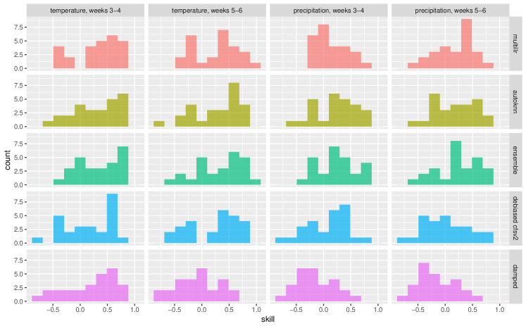
Figure 1. Distribution of contest-period skills of the proposed models MultiLLR and AutoKNN, the proposed ensemble of MultiLLR and AutoKNN (ensemble), the official contest debiased-CFSv2 baseline, and the official contest damped-persistence baseline (damped). See Section 5.2 for more details.

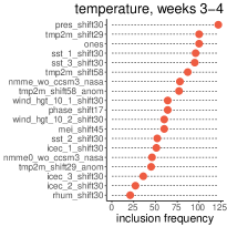
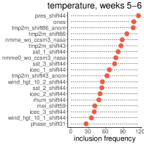
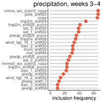
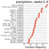
Figure 2. Feature inclusion frequencies of all candidate variables for local linear regression with multitask feature selection (MultiLLR) across all target dates in the historical forecast evaluation period (see Section 5.4).

5.3. Historical Forecast Evaluation

Next, we evaluate the performance of our methods over each year following the climatology period. That is, following the template of the contest period, we associate with each year in 2011-2017 a sequence of biweekly forecast issue dates between April 18 of that year and April 17 of the following year. For example, forecasts with submission dates between April 18, 2011 and April 17, 2012 are considered to belong to the evaluation year 2011. To mimic the actual real-time use of the forecasting system to produce forecasts for a particular target date, we train our models using only data available prior to the forecast issue date; for example, the forecasts issued on April 18, 2011 are only trained on data available prior to April 18, 2011. We compare our methods to the reconstructed debiased CFSv2 forecast.

Table 2 shows the average skills of our methods and the reconstructed debiased CFSv2 forecast (denoted by rec-deb-cfs) in each year, 2011-2017. MultiLLR, AutoKNN, and the ensemble all achieve higher average skill than debiased CFSv2 on every task, save for MultiLLR on the temperature, weeks 3-4 task. The ensemble improves over the debiased CFSv2 average skill by 23% for temperature weeks 3-4, by 39% for temperature weeks 5-6, by 123% for precipitation weeks 3-4, and by 157% for precipitation weeks 5-6.

Table 2 also presents the average skills achieved by a three-component ensemble of MultiLLR, AutoKNN, and reconstructed debiased CFSv2. Guided by Proposition 1, we $\ell_{2}$-normalize the anomalies of each model before taking an equal-weighted average. This ensemble (denoted by ens-cfs) produces higher average skills than the original ensemble in all prediction tasks. The ens-cfs ensemble also substantially outperforms debiased CFSv2, with skill improvements of 40% and 50% for the temperature tasks and 129% and 169% for the precipitation tasks. These results highlight the valuable roles that ML-based models, physics-based models, and principled ensembling can all play in subseasonal forecasting.

Contribution of NMME

Interestingly, the skill improvements of AutoKNN were achieved without any use of physics-based model forecasts. Moreover, a Proposition 1 ensemble of just AutoKNN and rec-deb-cfsv2 realizes most of the gains of ens-cfs without using NMME. Indeed, this ensemble has mean skills over all years in Table 2 of (temp. weeks 3-4: 0.354, temp. weeks 5-6: 0.31, precip. weeks 3-4: 0.162, precip. weeks 5-6: 0.147).

While physics-based model forecasts contribute to MultiLLR through the NMME ensemble mean, nmme_wo_ccsm3_nasa alone achieves inferior mean skill (temp. weeks 3-4: 0.094, temp. weeks 5-6: 0.116, precip. weeks 3-4: 0.116, precip. weeks 5-6: 0.107) over all years in Table 2 than all proposed methods and even the temperature debiased CFSv2 baseline. One contributing factor to this performance is the mismatch between the monthly granularity of the publicly-available NMME forecasts and the biweekly granularity of our forecast periods. As a result, we anticipate that more granular NMME data would lead to significant improvements in the final MultiLLR model.

Table 2. Average skills for historical forecasts in each year following the climatology period (see Section 5.3). We compare the proposed models MultiLLR and AutoKNN, the proposed ensemble of MultiLLR and AutoKNN (ensemble), the reconstructed debiased CFSv2 baseline (rec-deb-cfs), and the proposed ensemble of MultiLLR, AutoKNN, and debiased CFSv2 (ens-cfs).

	temperature, weeks 3-4					temperature, weeks 5-6
year	multillr	autoknn	ensemble	rec-deb-cfs	ens-cfs	multillr	autoknn	ensemble	rec-deb-cfs	ens-cfs
2011	0.2695	0.3664	0.3525	0.4598	0.4589	0.2522	0.3240	0.3537	0.3879	0.4284
2012	0.1466	0.3135	0.2548	0.1397	0.2505	0.2313	0.3205	0.3193	0.1030	0.3033
2013	0.1031	0.2011	0.1852	0.2861	0.2878	0.2212	0.0531	0.1833	0.1211	0.1828
2014	0.1973	0.2775	0.2935	0.3018	0.3547	0.1585	0.3056	0.2643	0.1936	0.3297
2015	0.3513	0.3885	0.4269	0.2857	0.4404	0.2694	0.3939	0.3752	0.4234	0.4426
2016	0.2654	0.3502	0.3467	0.2490	0.3839	0.2213	0.2882	0.2933	0.0983	0.2720
2017	0.3079	0.2807	0.3451	0.0676	0.3253	0.2562	0.2817	0.3025	0.1708	0.3003
all	0.2344	0.3111	0.3150	0.2557	0.3573	0.2300	0.2810	0.2988	0.2142	0.3221

	precipitation, weeks 3-4					precipitation, weeks 5-6
year	multillr	autoknn	ensemble	rec-deb-cfs	ens-cfs	multillr	autoknn	ensemble	rec-deb-cfs	ens-cfs
2011	0.1817	0.2173	0.2420	0.1646	0.2692	0.1398	0.2132	0.2210	0.1835	0.2666
2012	0.3147	0.3648	0.3983	0.0828	0.3909	0.3039	0.3943	0.4002	0.1941	0.4224
2013	0.1552	0.2026	0.2130	0.0648	0.1711	0.1392	0.1784	0.2031	0.0782	0.1939
2014	0.0790	0.1208	0.1391	0.1272	0.1738	​​-0.0069	0.0818	0.0556	0.0155	0.0782
2015	0.0645	​​-0.0053	0.0532	0.0837	0.1043	0.0802	0.0204	0.0755	0.0292	0.0959
2016	0.1419	​​-0.0568	0.0636	0.0190	0.0435	0.1703	​​-0.0930	0.0569	​​-0.0160	0.0483
2017	0.1597	0.2156	0.2364	0.0596	0.2250	0.1876	0.1870	0.2315	​​-0.0038	0.1978
all	0.1567	0.1513	0.1922	0.0860	0.1968	0.1449	0.1403	0.1777	0.0691	0.1857

5.4. Exploring MultiLLR

Fig. 2 shows the frequency with which each candidate feature was selected by MultiLLR in the four prediction tasks, across all target dates in the historical evaluation period. For all four tasks, the most frequently selected features include pressure (pres), the intercept term (ones), and temperature (tmp2m). The NMME ensemble average (nmme_wo_ccsm3_nasa) is the first or second most commonly selected feature for predicting precipitation, but its relative selection frequency is much lower for temperature.

Although we used a slightly larger set of candidate features for the precipitation tasks—23 for precipitation, compared to 20 for temperature—the selected models are more parsimonious for precipitation than for temperature. The median number of selected features for predicting temperature is 7 for both forecasting horizons, while the median number of selected features for predicting precipitation is 4 for weeks 3-4 and 5 for weeks 5-6.

5.5. Exploring AutoKNN

Fig. 3(a) plots the month distribution of the top nearest neighbor learned by AutoKNN for predicting precipitation, weeks 3-4, as a function of the month of the target date. The figure shows that when predicting precipitation, the top neighbor for a target date is generally from the same time of year as the target date: for summer target dates, the top neighbor tends to be from a summer month and similarly for winter target dates. The corresponding plot for temperature (omitted due to space constraints) shows that this pattern does not hold when predicting temperature; rather, the top neighbors are drawn from throughout the year, regardless of the month of the target date.

The matrix plots in Fig. 3(b) show the year and month of the top 20 nearest neighbors for predicting temperature, weeks 3-4, as a function of the target date. In each plot, the vertical axis ranges from $k=1$ (most similar neighbor) to $k=20$ (20th most similar neighbor). The vertical striations in both plots indicate that the top 20 neighbors for a given target date tend to be homogeneous in terms of both month and year: neighbors tend to come from the same or adjacent years and times of year. Moreover. the neighbors for post-2015 target dates tend to be from post-2010 years, in keeping with recent years’ record high temperatures. The corresponding plots for precipitation (omitted due to space constraints) show that the top neighbors for precipitation do not disproportionately come from recent years, and the months of the top neighbors follow a regular seasonal pattern, consistent with Fig. 3(a).

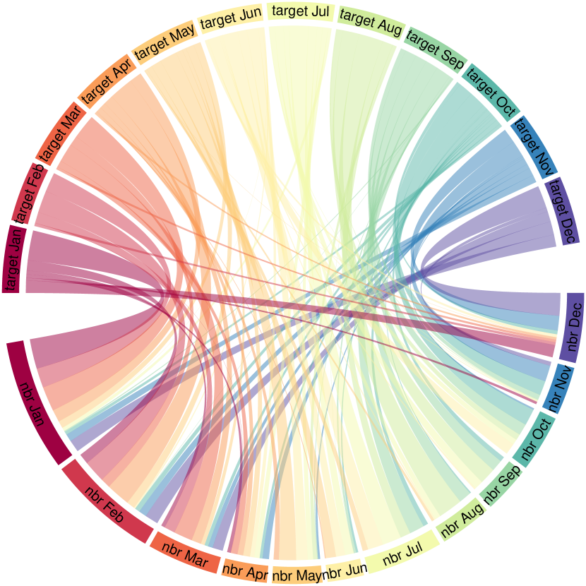
(a)

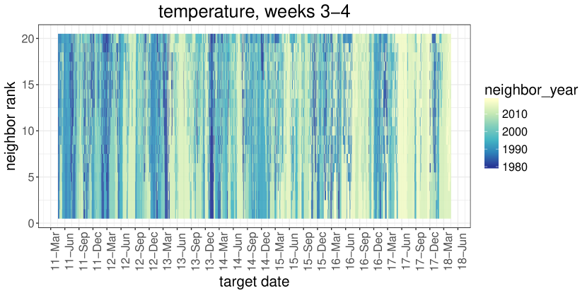
(b)

Figure 3. (a) Precipitation, weeks 3-4: Distribution of the month of the most similar neighbor learned by AutoKNN as a function of the month of the target date. (b) Temperature, weeks 3-4: Year (top) and month (bottom) of the 20 most similar neighbors learned by AutoKNN (vertical axis ranges from $k=1$ to $20$) as a function of the target date (horizontal axis).

6. Discussion

To meet the USBR’s Subseasonal Climate Forecast Rodeo challenge, we developed an ML-based forecasting system and demonstrated 40-169% improvements in forecasting skill across the challenge period (2017-18) and the years 2011-18 more generally. Notably, the same procedures provide these improvements for each of the four Rodeo prediction tasks (forecasting temperature or precipitation at weeks 3-4 or weeks 5-6). In the short term, we anticipate that these improvements will benefit disaster management (e.g., anticipating droughts, floods, and other wet weather extremes) and the water management, development, and protection operations of the USBR more generally (e.g., providing irrigation water to 20% of western U.S. farmers and generating hydroelectricity for 3.5 million homes). In the longer term, we hope that these tools will improve our ability to anticipate and manage wildfires (White et al., 2017).

Our experience also suggests that subseasonal forecasting is fertile ground for machine learning development. Much of the methodological novelty in our approach was driven by the unusual multitask forecasting skill objective. This objective inspired our new and provably beneficial ensembling approach and our custom multitask neighbor selection strategy. We hope that introducing this problem to the ML community and providing a user-friendly benchmark dataset will stimulate the development and evaluation of additional subseasonal forecasting approaches.

Appendix A Supplementary SubseasonalRodeo Dataset Details

The SubseasonalRodeo dataset is organized as a collection of Python Pandas DataFrames and Series objects (McKinney, 2010) stored in HDF5 format (via pandas.DataFrame.to_hdf or pandas.Series.to_hdf), with one .h5 file per DataFrame or Series. The contents of any file can be loaded in Python using pandas.read_hdf. Each DataFrame or Series contributes data variables (features or target values) falling into one of three categories: (i) spatial (varying with the target grid point but not the target date); (ii) temporal (varying with the target date but not the target grid point); (iii) spatiotemporal (varying with both the target grid point and the target date). Unless otherwise noted in Section 3 or below, temporal and spatiotemporal variables arising from daily data sources were derived by averaging input values over each 14-day period, and spatial and spatiotemporal variables were derived by interpolating input data to a $1^{\circ}\times 1^{\circ}$ grid using the Climate Data Operators (CDO version 1.8.2) operator remapdis (distance-weighted average interpolation) with target grid r360x181 and retaining only the contest grid points. In addition to the variables described in Section 3, a number of auxiliary variables were downloaded and processed but not ultimately used in our approach.

A.1. Temperature and Precipitation Interpolation

The downloaded temperature variables tmin and tmax, global precipitation variable rain, and U.S. precipitation variable precip were each interpolated to a fixed $1^{\circ}\times 1^{\circ}$ grid using the NCAR Command Language (NCL version 6.0.0) function area_hi2lores_Wrap with arguments new_lat = latGlobeF(181, "lat", "latitude", "degrees_north"); new_lon = lonGlobeF(360, "lon", "longitude", "degrees_east"); wgt = cos(lat*pi/180.0) (so that points are weighted by the cosine of the latitude in radians); opt@critpc = 50 (to require only 50% of the values to be present to interpolate); and fiCyclic = True (indicating global data with longitude values that do not quite wrap around the globe). rain was then renamed to precip.

A.2. Data Sources

The SubseasonalRodeo dataset data were downloaded from the following sources.

• Temperature (Fan and van den Dool, 2008): ftp://ftp.cpc.ncep.noaa.gov/precip/PEOPLE/wd52ws/global_temp/

• Global precipitation (Xie et al., 2010): ftp://ftp.cpc.ncep.noaa.gov/precip/CPC_UNI_PRCP/GAUGE_GLB/RT/

• U.S. precipitation (Xie et al., 2010): https://www.esrl.noaa.gov/psd/thredds/catalog/Datasets/cpc_us_precip/catalog.html

• Sea surface temperature and sea ice concentration (Reynolds et al., 2007): ftp://ftp.cdc.noaa.gov/Projects/Datasets/noaa.oisst.v2.highres/

• Multivariate ENSO index (MEI) (Wolter, 1993; Wolter and Timlin, 1998; Zimmerman et al., 2016): https://www.esrl.noaa.gov/psd/enso/mei/

• Madden-Julian oscillation (MJO) (Wheeler and Hendon, 2004): http://www.bom.gov.au/climate/mjo/graphics/rmm.74toRealtime.txt

• Relative humidity, sea level pressure, and precipitable water for entire atmosphere (Kalnay et al., 1996): ftp://ftp.cdc.noaa.gov/Datasets/ncep.reanalysis/surface/

• Pressure and potential evaporation (Kalnay et al., 1996): ftp://ftp.cdc.noaa.gov/Datasets/ncep.reanalysis/surface_gauss/

• Geopotential height, zonal wind, and longitudinal wind (Kalnay et al., 1996): ftp://ftp.cdc.noaa.gov/Datasets/ncep.reanalysis.dailyavgs/pressure/

• North American Multi-Model Ensemble (NMME) (Kirtman et al., 2014): https://iridl.ldeo.columbia.edu/SOURCES/.Models/.NMME/

• Elevation (Gates and Nelson, 1975): http://research.jisao.washington.edu/data_sets/elevation/elev.1-deg.nc

• Köppen-Geiger climate classifications (Kottek et al., 2006): http://koeppen-geiger.vu-wien.ac.at/present.htm

A.3. Dataset Files

Below, we list the contents of each SubseasonalRodeo dataset file. Each file with the designation ‘Series’ contains a Pandas Series object with a MultiIndex for the target latitude (lat), longitude (lon), and date defining the start of the target two-week period (start_date). Each file with the designation ‘MultiIndex DataFrame’ contains a Pandas DataFrame object with a MultiIndex for lat, lon, and start_date. Each file with a filename beginning with ‘nmme’ contains a Pandas DataFrame object with target_start, lat, and lon columns; the target_start column plays the same role as start_date in other files, indicating the date defining the start of the target two-week period. Each remaining file with the designation ‘DataFrame’ contains a Pandas DataFrame object with lat and lon columns if the contained variables are spatial; a start_date column if the contained variables are temporal; and start_date, lat, and lon columns if the contained variables are spatiotemporal.

The filename prefix ‘gt-wide’ indicates that a file contains temporal variables representing a base variable’s measurement at multiple locations on a latitude-longitude grid that need not correspond to contest grid point locations. The temporal variable column names are tuples in the format (‘base variable name’, latitude, longitude). The base variable measurements underlying the files with the filename prefix ‘gt-wide_contest’ were first interpolated to a $1^{\circ}\times 1^{\circ}$ grid. The measurements underlying the remaining ‘gt-wide’ files did not undergo interpolation; the original data source grids were instead employed.

• gt-climate_regions.h5 (DataFrame)

  • Spatial variable Köppen-Geiger climate classifications (climate_region)

• gt-contest_pevpr.sfc.gauss-14d-1948-2018.h5 (Series)

  • Spatiotemporal variable potential evaporation (pevpr.sfc.gauss)

• gt-contest_precip-14d-1948-2018.h5 (Series)

  • Spatiotemporal variable precipitation (precip)

• gt-contest_pres.sfc.gauss-14d-1948-2018.h5 (Series)

  • Spatiotemporal variable pressure (pres.sfc.gauss)

• gt-contest_pr_wtr.eatm-14d-1948-2018.h5 (Series)

  • Spatiotemporal variable precipitable water for entire atmosphere (pr_wtr.eatm)

• gt-contest_rhum.sig995-14d-1948-2018.h5 (Series)

  • Spatiotemporal variable relative humidity (rhum.sig995)

• gt-contest_slp-14d-1948-2018.h5 (Series)

  • Spatiotemporal variable sea level pressure (slp)

• gt-contest_tmax-14d-1979-2018.h5 (Series)

  • Spatiotemporal variable maximum temperature at 2m (tmax)

• gt-contest_tmin-14d-1979-2018.h5 (Series)

  • Spatiotemporal variable minimum temperature at 2m (tmin)

• gt-contest_tmp2m-14d-1979-2018.h5 (DataFrame)

  • Spatiotemporal variables temperature at 2m (tmp2m), average squared temperature at 2m over two-week period (tmp2m_sqd), and standard deviation of temperature at 2m over two-week period (tmp2m_std)

• gt-contest_wind_hgt_100-14d-1948-2018.h5 (Series)

  • Spatiotemporal variable geopotential height at 100 millibars (contest_wind_hgt_100)

• gt-contest_wind_hgt_10-14d-1948-2018.h5 (Series)

  • Spatiotemporal variable geopotential height at 10 millibars (contest_wind_hgt_10)

• gt-contest_wind_hgt_500-14d-1948-2018.h5 (Series)

  • Spatiotemporal variable geopotential height at 500 millibars (contest_wind_hgt_500)

• gt-contest_wind_hgt_850-14d-1948-2018.h5 (Series)

  • Spatiotemporal variable geopotential height at 850 millibars (contest_wind_hgt_850)

• gt-contest_wind_uwnd_250-14d-1948-2018.h5 (Series)

  • Spatiotemporal variable zonal wind at 250 millibars (contest_wind_uwnd_250)

• gt-contest_wind_uwnd_925-14d-1948-2018.h5 (Series)

  • Spatiotemporal variable zonal wind at 925 millibars (contest_wind_uwnd_925)

• gt-contest_wind_vwnd_250-14d-1948-2018.h5 (Series)

  • Spatiotemporal variable longitudinal wind at 250 millibars (contest_wind_vwnd_250)

• gt-contest_wind_vwnd_925-14d-1948-2018.h5 (Series)

  • Spatiotemporal variable longitudinal wind at 925 millibars (contest_wind_vwnd_925)

• gt-elevation.h5 (DataFrame)

  • Spatial variable elevation (elevation)

• gt-mei-1950-2018.h5 (DataFrame)

  • Temporal variables MEI (mei), MEI rank (rank), and Niño Index Phase (nip) derived from mei and rank using the definition in (Zimmerman et al., 2016)

• gt-mjo-1d-1974-2018.h5 (DataFrame)

  • Temporal variables MJO phase (phase) and amplitude (amplitude)

• gt-pca_icec_2010-14d-1981-2018.h5 (DataFrame)

  • Temporal variables top PCs of gt-wide_contest_icec-14d-1981-2018.h5 based on PC loadings from 1981-2010

• gt-pca_sst_2010-14d-1981-2018.h5 (DataFrame)

  • Temporal variables top PCs of gt-wide_contest_sst-14d-1981-2018.h5 based on PC loadings from 1981-2010

• gt-pca_wind_hgt_100_2010-14d-1948-2018.h5 (DataFrame)

  • Temporal variables top PCs of gt-wide_wind_hgt_100-14d-1948-2018.h5 based on PC loadings from 1948-2010

• gt-pca_wind_hgt_10_2010-14d-1948-2018.h5 (DataFrame)

  • Temporal variables top PCs of gt-wide_wind_hgt_10-14d-1948-2018.h5 based on PC loadings from 1948-2010

• gt-pca_wind_hgt_500_2010-14d-1948-2018.h5 (DataFrame)

  • Temporal variables top PCs of gt-wide_wind_hgt_500-14d-1948-2018.h5 based on PC loadings from 1948-2010

• gt-pca_wind_hgt_850_2010-14d-1948-2018.h5 (DataFrame)

  • Temporal variables top PCs of gt-wide_wind_hgt_850-14d-1948-2018.h5 based on PC loadings from 1948-2010

• gt-pca_wind_uwnd_250_2010-14d-1948-2018.h5 (DataFrame)

  • Temporal variables top PCs of gt-wide_wind_uwnd_250-14d-1948-2018.h5 based on PC loadings from 1948-2010

• gt-pca_wind_uwnd_925_2010-14d-1948-2018.h5 (DataFrame)

  • Temporal variables top PCs of gt-wide_wind_uwnd_925-14d-1948-2018.h5 based on PC loadings from 1948-2010

• gt-pca_wind_vwnd_250_2010-14d-1948-2018.h5 (DataFrame)

  • Temporal variables top PCs of gt-wide_wind_vwnd_250-14d-1948-2018.h5 based on PC loadings from 1948-2010

• gt-pca_wind_vwnd_925_2010-14d-1948-2018.h5 (DataFrame)

  • Temporal variables top PCs of gt-wide_wind_vwnd_925-14d-1948-2018.h5 based on PC loadings from 1948-2010

• gt-wide_contest_icec-14d-1981-2018.h5 (DataFrame)

  • Temporal variables sea ice concentration for all grid points in the Pacific basin (20S to 65N, 150E to 90W) ((‘icec’,latitude,longitude))

• gt-wide_contest_sst-14d-1981-2018.h5 (DataFrame)

  • Temporal variables sea surface temperature for all grid points in the Pacific basin (20S to 65N, 150E to 90W) ((‘sst’,latitude,longitude))

• gt-wide_wind_hgt_100-14d-1948-2018.h5 (DataFrame)

  • Temporal variables geopotential height at 100 millibars for all grid points globally ((‘wind_hgt_100’,latitude,longitude))

• gt-wide_wind_hgt_10-14d-1948-2018.h5 (DataFrame)

  • Temporal variables geopotential height at 10 millibars for all grid points globally ((‘wind_hgt_10’,latitude,longitude))

• gt-wide_wind_hgt_500-14d-1948-2018.h5 (DataFrame)

  • Temporal variables geopotential height at 500 millibars for all grid points globally ((‘wind_hgt_500’,latitude,longitude))

• gt-wide_wind_hgt_850-14d-1948-2018.h5 (DataFrame)

  • Temporal variables geopotential height at 850 millibars for all grid points globally ((‘wind_hgt_850’,latitude,longitude))

• gt-wide_wind_uwnd_250-14d-1948-2018.h5 (DataFrame)

  • Temporal variables zonal wind at 250 millibars for all grid points globally ((‘wind_uwnd_250’,latitude,longitude))

• gt-wide_wind_uwnd_925-14d-1948-2018.h5 (DataFrame)

  • Temporal variables zonal wind at 925 millibars for all grid points globally ((‘wind_uwnd_925’,latitude,longitude))

• gt-wide_wind_vwnd_250-14d-1948-2018.h5 (DataFrame)

  • Temporal variables longitudinal wind at 250 millibars for all grid points globally ((‘wind_vwnd_250’,latitude,longitude))

• gt-wide_wind_vwnd_925-14d-1948-2018.h5 (DataFrame)

  • Temporal variables longitudinal wind at 925 millibars for all grid points globally ((‘wind_vwnd_925’,latitude,longitude))

• nmme0-prate-34w-1982-2018.h5 (DataFrame)

  • Spatiotemporal variables most recent monthly NMME model forecasts for precip (cancm3_0, cancm4_0, ccsm3_0, ccsm4_0, cfsv2_0, gfdl-flor-a_0, gfdl-flor-b_0, gfdl_0, ’nasa_0, ’nmme0_mean) and average forecast across those models (nmme0_mean)

• nmme0-prate-56w-1982-2018.h5 (DataFrame)

  • Spatiotemporal variables most recent monthly NMME model forecasts for precip (cancm3_0, cancm4_0, ccsm3_0, ccsm4_0, cfsv2_0, gfdl-flor-a_0, gfdl-flor-b_0, gfdl_0, ’nasa_0, ’nmme0_mean) and average forecast across those models (nmme0_mean)

• nmme0-tmp2m-34w-1982-2018.h5 (DataFrame)

  • Spatiotemporal variables most recent monthly NMME model forecasts for tmp2m (cancm3_0, cancm4_0, ccsm3_0, ccsm4_0, cfsv2_0, gfdl-flor-a_0, gfdl-flor-b_0, gfdl_0, ’nasa_0, ’nmme0_mean) and average forecast across those models (nmme0_mean)

• nmme0-tmp2m-56w-1982-2018.h5 (DataFrame)

  • Spatiotemporal variables most recent monthly NMME model forecasts for tmp2m (cancm3_0, cancm4_0, ccsm3_0, ccsm4_0, cfsv2_0, gfdl-flor-a_0, gfdl-flor-b_0, gfdl_0, ’nasa_0, ’nmme0_mean) and average forecast across those models (nmme0_mean)

• nmme-prate-34w-1982-2018.h5 (DataFrame)

  • Spatiotemporal variables weeks 3-4 weighted average of monthly NMME model forecasts for precip (cancm3, cancm4, ccsm3, ccsm4, cfsv2, gfdl, gfdl-flor-a, gfdl-flor-b, nasa) and average forecast across those models (nmme_mean)

• nmme-prate-56w-1982-2018.h5 (DataFrame)

  • Spatiotemporal variables weeks 5-6 weighted average of monthly NMME model forecasts for precip (cancm3, cancm4, ccsm3, ccsm4, cfsv2, gfdl, gfdl-flor-a, gfdl-flor-b, nasa) and average forecast across those models (nmme_mean)

• nmme-tmp2m-34w-1982-2018.h5 (DataFrame)

  • Spatiotemporal variables weeks 3-4 weighted average of monthly NMME model forecasts for tmp2m (cancm3, cancm4, ccsm3, ccsm4, cfsv2, gfdl, gfdl-flor-a, gfdl-flor-b, nasa) and average forecast across those models (nmme_mean)

• nmme-tmp2m-56w-1982-2018.h5 (DataFrame)

  • Spatiotemporal variables weeks 5-6 weighted average of monthly NMME model forecasts for tmp2m (cancm3, cancm4, ccsm3, ccsm4, cfsv2, gfdl, gfdl-flor-a, gfdl-flor-b, nasa) and average forecast across those models (nmme_mean)

• official_climatology-contest_precip-1981-2010.h5 (DataFrame)

  • Spatiotemporal variable precipitation climatology (precip_clim). Only the dates 1799-12-19–1800-12-18 are included as representatives of each (non-leap day) month-day combination.

• official_climatology-contest_tmp2m-1981-2010.h5 (DataFrame)

  • Spatiotemporal variable temperature at 2 meters climatology (tmp2m_clim). Only the dates 1799-12-19–1800-12-18 are included as representatives of each (non-leap day) month-day combination.

Appendix B Debiased CFSv2 Reconstruction Details

For the target dates in the 2011-2018 historical forecast evaluation period of Section 5.3, Climate Forecast System (CFSv2) archived operational forecasts were retrieved from the National Center for Environmental Information (NCEI) site at https://nomads.ncdc.noaa.gov/modeldata/cfsv2_forecast_ts_9mon/. The Gaussian gridded data (approximately 0.93^∘ resolution) for precipitation rate and 2-meter temperature were interpolated to the Rodeo forecast grid at 1^∘ resolution. These data were then extracted as a window from 25 to 50 N and -125 to -93 W. Data were extracted for all forecast issue dates, for each cardinal hour (00, 06, 12, and 18 UTC). Interpolation from Gaussian grid to regular $1^{\circ}\times 1^{\circ}$ latitude longitude grids was accomplished using a bilinear interpolation under the Python Basemap package (Hunter, 2007). Any missing data were replaced by the average measurement from the available forecasts in the 2-week period.

To obtain a suitable long-term average for debiasing our reconstructed CFSv2 forecasts, precipitation (prate_f) and temperature (tmp2m_f) CFS Reforecast data from 1999-2010 were downloaded from https://nomads.ncdc.noaa.gov/data/cfsr-hpr-ts45/; interpolated to a $1^{\circ}\times 1^{\circ}$ grid via bilinear interpolation using wgrib2 (v0.2.0.6c) with arguments -new_grid_winds earth and -new_grid ncep grid 3; and then restricted to the contest region. Temperatures were converted from Kelvin to Celsius, and the precipitation measurements were scaled from mm/s to mm/2-week period. Finally, each 2-week period in the data was averaged (for temperature) or summed (for precipitation). Any missing data were replaced by the average measurement from the available forecasts in the 2-week period.

arxiv

Appendix C Supplementary Figures

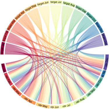
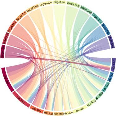
Figure 4. Distribution of the month of the most similar neighbor learned by AutoKNN as a function of the month of the target date to be predicted. Left: Most similar neighbor for temperature, weeks 3-4. Right: Most similar neighbor for precipitation, weeks 3-4. The plots for weeks 5-6 are very similar. For temperature, the most similar neighbor can come from any time of year, regardless of the month of the target date. For precipitation, we instead observe a strong seasonal pattern; the season of the most similar neighbor generally matches the season of the target date.

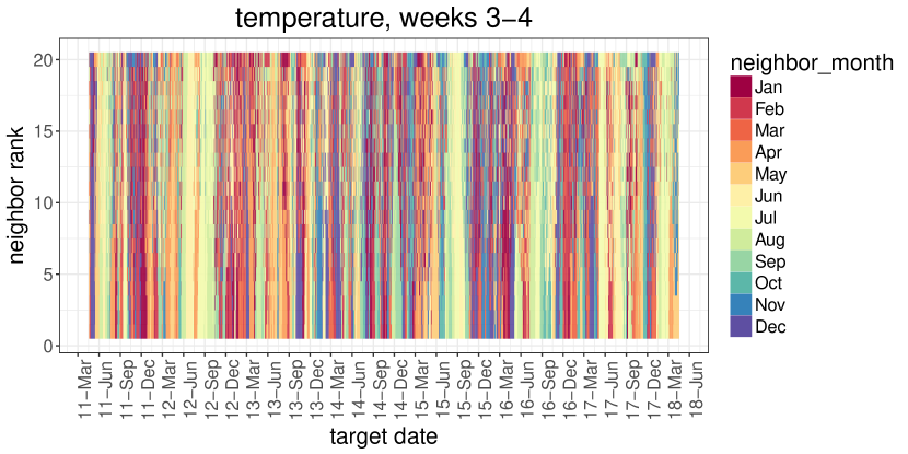
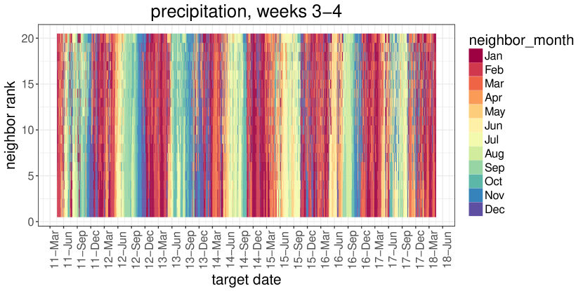
Figure 5. Month of the 20 most similar neighbors learned by AutoKNN (vertical axis ranges from $k=1$ to $20$) as a function of the target date to be predicted (horizontal axis). The plots for weeks 5-6 are very similar. Both temperature and precipitation neighbors are homogeneous in month for a given target date, but the months of the precipitation neighbors also exhibit a regular seasonal pattern from year to year, while the temperature neighbors do not.

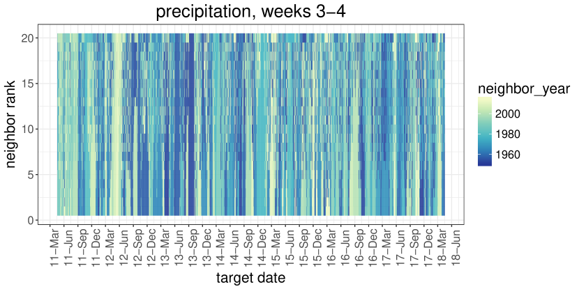
Figure 6. Year of the 20 most similar neighbors learned by AutoKNN (vertical axis ranges from $k=1$ to $20$) as a function of the target date to be predicted (horizontal axis). The plots for weeks 5-6 are very similar. The temperature neighbors are disproportionately drawn from recent years (post-2010), while the precipitation neighbors are not.

References

- (1)
- Badr et al. (2014) Hamada S. Badr, Benjamin F. Zaitchik, and Seth D. Guikema. 2014. Application of Statistical Models to the Prediction of Seasonal Rainfall Anomalies over the Sahel. Journal of Applied Meteorology and Climatology 53, 3 (2014), 614–636. DOI:http://dx.doi.org/10.1175/JAMC-D-13-0181.1
- Barnston et al. (2012) Anthony G Barnston, Michael K Tippett, Michelle L L’Heureux, Shuhua Li, and David G DeWitt. 2012. Skill of real-time seasonal ENSO model predictions during 2002–11: Is our capability increasing? Bulletin of the American Meteorological Society 93, 5 (2012), 631–651.
- Cofino et al. (2002) Antonio S Cofino, Rafael Cano Trueba, Carmen María Sordo, and José Manuel Gutiérrez Llorente. 2002. Bayesian networks for probabilistic weather prediction. (2002).
- Cohen et al. (2019) Judah Cohen, Dim Coumou, Jessica Hwang, Lester Mackey, Paulo Orenstein, Sonja Totz, and Eli Tziperman. 2019. S2S reboot: An argument for greater inclusion of machine learning in subseasonal to seasonal forecasts. Wiley Interdisciplinary Reviews: Climate Change 10, 2 (2019), e00567.
- Fan and van den Dool (2008) Yun Fan and Huug van den Dool. 2008. A global monthly land surface air temperature analysis for 1948-present. Journal of Geophysical Research: Atmospheres 113, D1 (2008). DOI:http://dx.doi.org/10.1029/2007JD008470
- Gates and Nelson (1975) William Lawrence Gates and Alfred B Nelson. 1975. A New (Revised) Tabulation of the Scripps Topography on a 1 degree Global Grid. Part 1. Terrain Heights. Technical Report. RAND CORP SANTA MONICA CA.
- Ghaderi et al. (2017) Amir Ghaderi, Borhan M Sanandaji, and Faezeh Ghaderi. 2017. Deep forecast: deep learning-based spatio-temporal forecasting. arXiv preprint arXiv:1707.08110 (2017).
- Ghosh and Krishnamurti (2018) T. Ghosh and T. N. Krishnamurti. 2018. Improvements in Hurricane Intensity Forecasts from a Multimodel Superensemble Utilizing a Generalized Neural Network Technique. Weather and Forecasting 33, 3 (2018), 873–885. DOI:http://dx.doi.org/10.1175/WAF-D-17-0006.1
- Grover et al. (2015) Aditya Grover, Ashish Kapoor, and Eric Horvitz. 2015. A deep hybrid model for weather forecasting. In Proceedings of the 21th ACM SIGKDD International Conference on Knowledge Discovery and Data Mining. ACM, 379–386.
- Herman and Schumacher (2018) Gregory R. Herman and Russ S. Schumacher. 2018. Dendrology in Numerical Weather Prediction: What Random Forests and Logistic Regression Tell Us about Forecasting Extreme Precipitation. Monthly Weather Review 146, 6 (2018), 1785–1812. DOI:http://dx.doi.org/10.1175/MWR-D-17-0307.1
- Hernández et al. (2016) Emilcy Hernández, Victor Sanchez-Anguix, Vicente Julian, Javier Palanca, and Néstor Duque. 2016. Rainfall prediction: A deep learning approach. In International Conference on Hybrid Artificial Intelligence Systems. Springer, 151–162.
- Horenko et al. (2008) Illia Horenko, Rupert Klein, Stamen Dolaptchiev, and Christof Schütte. 2008. Automated generation of reduced stochastic weather models i: simultaneous dimension and model reduction for time series analysis. Multiscale Modeling & Simulation 6, 4 (2008), 1125–1145.
- Hunter (2007) John D Hunter. 2007. Matplotlib: A 2D graphics environment. Computing in Science & Engineering 9, 3 (2007), 90–95.
- Hwang et al. (2018) Jessica Hwang, Paulo Orenstein, Judah Cohen, and Lester Mackey. 2018. The SubseasonalRodeo Dataset. (2018). DOI:http://dx.doi.org/10.7910/DVN/IHBANG Harvard Dataverse.
- Hwang et al. (2019) Jessica Hwang, Paulo Orenstein, Judah Cohen, Karl Pfeiffer, and Lester Mackey. 2019. Reconstructed Precipitation and Temperature CFSv2 Forecasts for 2011-2018. (2019). DOI:http://dx.doi.org/10.7910/DVN/CEFZLV Harvard Dataverse.
- Iglesias et al. (2015) Gilberto Iglesias, David C Kale, and Yan Liu. 2015. An examination of deep learning for extreme climate pattern analysis. In The 5th International Workshop on Climate Informatics.
- Kalnay et al. (1996) Eugenia Kalnay, Masao Kanamitsu, Robert Kistler, William Collins, Dennis Deaven, Lev Gandin, Mark Iredell, Suranjana Saha, Glenn White, John Woollen, and others. 1996. The NCEP/NCAR 40-year reanalysis project. Bulletin of the American Meteorological Society 77, 3 (1996), 437–472.
- Karevan and Suykens (2016) Zahra Karevan and Johan Suykens. 2016. Spatio-temporal feature selection for black-box weather forecasting. In Proc. of the 24th european symposium on artificial neural networks, computational intelligence and machine learning. 611–616.
- Karstens et al. (2018) Christopher D. Karstens, James Correia, Daphne S. LaDue, Jonathan Wolfe, Tiffany C. Meyer, David R. Harrison, John L. Cintineo, Kristin M. Calhoun, Travis M. Smith, Alan E. Gerard, and Lans P. Rothfusz. 2018. Development of a Human-Machine Mix for Forecasting Severe Convective Events. Weather and Forecasting 33, 3 (2018), 715–737. DOI:http://dx.doi.org/10.1175/WAF-D-17-0188.1
- Kirtman et al. (2014) Ben P Kirtman, Dughong Min, Johnna M Infanti, James L Kinter III, Daniel A Paolino, Qin Zhang, Huug Van Den Dool, Suranjana Saha, Malaquias Pena Mendez, Emily Becker, and others. 2014. The North American multimodel ensemble: phase-1 seasonal-to-interannual prediction; phase-2 toward developing intraseasonal prediction. Bulletin of the American Meteorological Society 95, 4 (2014), 585–601.
- Kottek et al. (2006) Markus Kottek, Jürgen Grieser, Christoph Beck, Bruno Rudolf, and Franz Rubel. 2006. World map of the Köppen-Geiger climate classification updated. Meteorologische Zeitschrift 15, 3 (2006), 259–263.
- Kuligowski and Barros (1998) Robert J Kuligowski and Ana P Barros. 1998. Localized precipitation forecasts from a numerical weather prediction model using artificial neural networks. Weather and forecasting 13, 4 (1998), 1194–1204.
- Liu et al. (2016) Yunjie Liu, Evan Racah, Joaquin Correa, Amir Khosrowshahi, David Lavers, Kenneth Kunkel, Michael Wehner, William Collins, and others. 2016. Application of deep convolutional neural networks for detecting extreme weather in climate datasets. arXiv preprint arXiv:1605.01156 (2016).
- Lorenz (1963) Edward N Lorenz. 1963. Deterministic nonperiodic flow. Journal of the Atmospheric Sciences 20, 2 (1963), 130–141.
- McGovern et al. (2014) Amy McGovern, David J Gagne, John K Williams, Rodger A Brown, and Jeffrey B Basara. 2014. Enhancing understanding and improving prediction of severe weather through spatiotemporal relational learning. Machine learning 95, 1 (2014), 27–50.
- McKinney (2010) Wes McKinney. 2010. Data structures for statistical computing in python. In Proceedings of the 9th Python in Science Conference, Vol. 445. Austin, TX, 51–56.
- Nebeker (1995) Frederik Nebeker. 1995. Calculating the weather: Meteorology in the 20th century. Vol. 60. Elsevier.
- Nowak et al. (2017) K Nowak, RS Webb, R Cifelli, and LD Brekke. 2017. Sub-Seasonal Climate Forecast Rodeo. In 2017 AGU Fall Meeting, New Orleans, LA, 11-15 Dec.
- Qiu et al. (2017) Minghui Qiu, Peilin Zhao, Ke Zhang, Jun Huang, Xing Shi, Xiaoguang Wang, and Wei Chu. 2017. A Short-Term Rainfall Prediction Model using Multi-Task Convolutional Neural Networks. In Data Mining (ICDM), 2017 IEEE International Conference on. IEEE, 395–404.
- Racah et al. (2017) Evan Racah, Christopher Beckham, Tegan Maharaj, Samira Ebrahimi Kahou, Mr Prabhat, and Chris Pal. 2017. ExtremeWeather: A large-scale climate dataset for semi-supervised detection, localization, and understanding of extreme weather events. In Advances in Neural Information Processing Systems. 3402–3413.
- Radhika and Shashi (2009) Y Radhika and M Shashi. 2009. Atmospheric temperature prediction using support vector machines. International Journal of Computer Theory and Engineering 1, 1 (2009), 55.
- Reynolds et al. (2007) Richard W Reynolds, Thomas M Smith, Chunying Liu, Dudley B Chelton, Kenneth S Casey, and Michael G Schlax. 2007. Daily high-resolution-blended analyses for sea surface temperature. Journal of Climate 20, 22 (2007), 5473–5496.
- Robertson et al. (2015) Andrew W. Robertson, Arun Kumar, Malaquias Peña, and Frederic Vitart. 2015. Improving and Promoting Subseasonal to Seasonal Prediction. Bulletin of the American Meteorological Society 96, 3 (2015), ES49–ES53. DOI:http://dx.doi.org/10.1175/BAMS-D-14-00139.1
- Saha et al. (2014) Suranjana Saha, Shrinivas Moorthi, Xingren Wu, Jiande Wang, Sudhir Nadiga, Patrick Tripp, David Behringer, Yu-Tai Hou, Hui-ya Chuang, Mark Iredell, and others. 2014. The NCEP climate forecast system version 2. Journal of Climate 27, 6 (2014), 2185–2208.
- Strobach and Bel (2016) Ehud Strobach and Golan Bel. 2016. Decadal Climate Predictions Using Sequential Learning Algorithms. Journal of Climate 29, 10 (2016), 3787–3809. DOI:http://dx.doi.org/10.1175/JCLI-D-15-0648.1
- Totz et al. (2017) Sonja Totz, Eli Tziperman, Dim Coumou, Karl Pfeiffer, and Judah Cohen. 2017. Winter Precipitation Forecast in the European and Mediterranean Regions Using Cluster Analysis. Geophysical Research Letters 44, 24 (2017), 12,418–12,426. DOI:http://dx.doi.org/10.1002/2017GL075674
- Vitart et al. (2012) Frédéric Vitart, Andrew W Robertson, and David LT Anderson. 2012. Subseasonal to Seasonal Prediction Project: Bridging the gap between weather and climate. Bulletin of the World Meteorological Organization 61, 2 (2012), 23.
- Wheeler and Hendon (2004) Matthew C Wheeler and Harry H Hendon. 2004. An all-season real-time multivariate MJO index: Development of an index for monitoring and prediction. Monthly Weather Review 132, 8 (2004), 1917–1932.
- White et al. (2017) Christopher J. White, Henrik Carlsen, Andrew W. Robertson, Richard J.T. Klein, Jeffrey K. Lazo, Arun Kumar, Frederic Vitart, Erin Coughlan de Perez, Andrea J. Ray, Virginia Murray, Sukaina Bharwani, Dave MacLeod, Rachel James, Lora Fleming, Andrew P. Morse, Bernd Eggen, Richard Graham, Erik Kjellstrom, Emily Becker, Kathleen V. Pegion, Neil J. Holbrook, Darryn McEvoy, Michael Depledge, Sarah Perkins-Kirkpatrick, Timothy J. Brown, Roger Street, Lindsey Jones, Tomas A. Remenyi, Indi Hodgson-Johnston, Carlo Buontempo, Rob Lamb, Holger Meinke, Berit Arheimer, and Stephen E. Zebiak. 2017. Potential applications of subseasonal-to-seasonal (S2S) predictions. Meteorological Applications 24, 3 (2017), 315–325. DOI:http://dx.doi.org/10.1002/met.1654
- Wolter (1993) Klaus Wolter. 1993. Monitoring ENSO in COADS with a seasonally adjusted principal component index. In Proc. of the 17th Climate Diagnostics Workshop, 1993.
- Wolter and Timlin (1998) Klaus Wolter and Michael S Timlin. 1998. Measuring the strength of ENSO events: How does 1997/98 rank? Weather 53, 9 (1998), 315–324.
- Xie et al. (2010) Pingping Xie, M Chen, and W Shi. 2010. CPC unified gauge-based analysis of global daily precipitation. In Preprints, 24th Conf. on Hydrology, Atlanta, GA, Amer. Meteor. Soc, Vol. 2.
- Xingjian et al. (2015) SHI Xingjian, Zhourong Chen, Hao Wang, Dit-Yan Yeung, Wai-Kin Wong, and Wang-chun Woo. 2015. Convolutional LSTM network: A machine learning approach for precipitation nowcasting. In Advances in neural information processing systems. 802–810.
- Zimmerman et al. (2016) Brian G. Zimmerman, Daniel J. Vimont, and Paul J. Block. 2016. Utilizing the state of ENSO as a means for season-ahead predictor selection. Water Resources Research 52, 5 (2016), 3761–3774. DOI:http://dx.doi.org/10.1002/2015WR017644