Hidden-Beauty Broad Resonance $Y_{b}(10890)$ in Thermal QCD

Abstract

In this work, the mass and pole residue of resonance $Y_{b}$ is studied by using QCD sum rules approach at finite temperature. Resonance $Y_{b}$ is described by a diquark-antidiquark tetraquark current, and contributions to operator product expansion are calculated by including QCD condensates up to dimension six. Temperature dependences of the mass $m_{Y_{b}}$ and the pole residue $\lambda_{Y_{b}}$ are investigated. It is seen that near a critical temperature $(T_{c}\simeq 190~{}\mathrm{MeV})$, the values of $m_{Y_{b}}$ and $\lambda_{Y_{b}}$ are decreased to $87\%$, and to $44\%$ of their values at vacuum.

1 Introduction

Heavy quarkonia systems provide a unique laboratory to search the interplay between perturbative and nonperturbative effects of QCD. They are non-relativistic systems in which low energy QCD can be investigated via their energy levels, widths, and transition amplitudes [1]. Among these heavy quarkonia states, vector charmonium and bottomonium sectors are experimentally studied very well, since they can be detected directly in $e^{+}e^{-}$ annihilations. In the past decade, observation of a large number of bottomonium-like states in several experiments increased the interest in these structures [2, 3, 4, 5, 6]. However, these observed states could not be conveniently explained by the simple $q\bar{q}$ picture of mesons. The presumption of hadrons containing quarks more than the standard quark content ($q\bar{q}$ or $qqq$) are introduced by a perceptible model for diquarks plus antidiquarks, which was developed by Jaffe in 1976 [7]. Later Maiani, Polosa and their collaborators proposed that the X, Y, Z mesons are tetraquark systems, in which the diquark-antidiquark pairs are bound together by the QCD color forces [8]. In this color configuration, diquarks can play a fundamental role in hadron spectroscopy. Thus, probing the multiquark matter has been an intensely intriguing research topic in the past twenty years and it may provide significant clues to understand the non-perturbative behavior of QCD.

In 2007, Belle reported the first evidence of $e^{+}e^{-}\rightarrow\Upsilon(1S)\pi^{+}\pi^{-},\Upsilon(2S)\pi^{+}\pi^{-}$ and first observation for $e^{+}e^{-}\rightarrow\Upsilon(3S)\pi^{+}\pi^{-},\Upsilon(1S)K^{+}K^{-}$ decays near the peak of the $\Upsilon(5S)$ state at $\sqrt{s}=10.87~{}\mathrm{GeV}$ [2]. Assigning these signals to $\Upsilon(5S)$, the partial widths of decays $\Upsilon(5S)\rightarrow\Upsilon(1S)\pi^{+}\pi^{-}$ and $\Upsilon(5S)\rightarrow\Upsilon(2S)\pi^{+}\pi^{-}$ were measured unusually larger (more than two orders of magnitude) than formerly measured decay widths of $\Upsilon(nS)$ states. Following these unusually large partial width measurement, Belle measured the cross sections of $e^{+}e^{-}\rightarrow\Upsilon(1S)\pi^{+}\pi^{-},\Upsilon(2S)\pi^{+}\pi^{-}$ and $\Upsilon(1S)\pi^{+}\pi^{-}$, and reported that the resonance observed via these decays does not agree with conventional $\Upsilon(5S)$ line shape. These observations led to the proposal of existence of new exotic hidden-beauty state analogous to broad $Y(4260)$ resonance in the charmonium sector, which is a Breit-Wigner shaped resonance with mass ($10888.4^{+2.7}_{-2.6}\pm 1.2$) MeV/c², and width ($30.7^{+8.3}_{-7.0}\pm 3.1$) MeV/c², and is called $Y_{b}(10890)$ [5]. In literature, there are several approaches to investigate the structure of exotic $Y_{b}$ resonance. In Ref. [9], $Y_{b}$ is considered as a $\Lambda_{b}\bar{\Lambda}_{b}$ bound state with an highly large binding energy. In Refs. [10, 11], $Y_{b}$ is interpreted as a tetraquark, and its mass is estimated by using QCD sum rules at vacuum.

Moreover, it is likely that at very high temperatures within the first microseconds following the Big Bang, quarks and gluons existed freely in a homogenous medium called the quark-gluon plasma (QGP). In 2011, CMS Collaboration reported that charmonium states $\phi(2S)$ and $J/\psi$ melt or be suppressed due to interacting with the hot nuclear matter created in heavy-ion interactions [12, 13]. Following these observations in the charmonium sector, CMS Collaboration also reported suppression of bottomonium states, $\Upsilon(2S)$ and $\Upsilon(3S)$ relative to the $\Upsilon(1S)$ ground state [14, 15]. The dissociation temperatures for the $\Upsilon$ states are expected to be related with their binding energies, and are predicted to be $2T_{c},~{}1.2T_{c}$ and $T_{c}$ for the $\Upsilon(1S),\Upsilon(2S)$, $2T_{c}$, and $Y(3S)$ mesons, respectively, where $T_{c}$ is the critical temperature for deconfinement [15, 16, 17]. Inspiring by these findings and motivated by the aforementioned discussions, we focus on the $Y_{b}$ resonance and its thermal behavior.

This paper is organized as follows. In section 2, theoretical framework of Thermal QCD sum rules (TQCDSR) and its application to $Y_{b}$ are presented, and obtained analytical expressions of the mass and pole residue of $Y_{b}$ are given up to dimension six operators. Numerical analysis is performed and results are obtained in section 3. Concluding remarks are discussed in section 4. The explicit forms of the spectral densities are written in Appendix.

2 Finite Temperature Sum Rules for Tetraquark Assignment

QCD sum rules (QCDSR) approach is based on Wilson’s operator product expansion (OPE) which was adapted by Shifman, Vainshtein and Zakharov, and applied with remarkable success to estimate a large variety of properties of all low-lying hadronic states [18, 19, 20, 21]. Later, this model is extended to its thermal version that is firstly proposed by Bochkarev and Shaposnikov, and led to many successful applications in QCD [22, 23, 24, 25, 26, 27, 28]. In this section, the mass and pole residue of the exotic $Y_{b}$ resonance are studied by interpreting it as a bound $[bs][\bar{b}\bar{s}]$ tetraquark via TQCDSR technique which starts with the two point correlation function

$$\Pi_{\mu\nu}(q,T)=i\int d^{4}x~{}e^{iq\cdot x}\langle\Psi|\mathcal{T}\{\eta_{\mu}(x)\eta_{\nu}^{\dagger}(0)\}|\Psi\rangle,$$ (1)

where $\Psi$ represents the hot medium state, $\eta_{\mu}(x)$ is the interpolating current of the $Y_{b}$ state and $\mathcal{T}$ denotes the time ordered product. The thermal average of any operator $\hat{O}$ in thermal equilibrium is given as

$$\langle\hat{O}\rangle=\frac{Tr(e^{-\beta\mathcal{H}}\hat{O})}{Tr(e^{-\beta\mathcal{H}})},\\$$ (2)

where $\mathcal{H}$ is the QCD Hamiltonian, and $\mathcal{\beta}=1/T$ is inverse of the temperature, and $T$ is the temperature of the heat bath. Chosen current $\eta_{\mu}(x)$ must contain all the information of the related meson, like quantum numbers, quark contents and so on. In the diquark-antidiquark picture, tetraquark current interpreting $Y_{b}$ can be chosen as [29]

$$\eta_{\mu}(x) = \frac{i\epsilon\tilde{\epsilon}}{\sqrt{2}}\Big{\{}\Big{[}~{}s_{a}^{T}(x)C\gamma_{5}b_{b}(x)\Big{]}\Big{[}~{}\overline{s}_{d}(x)\gamma_{\mu}\gamma_{5}C\overline{b}_{e}^{T}(x)\Big{]}$$ (3)

$$+ \Big{[}~{}s_{a}^{T}(x)C\gamma_{5}\gamma_{\mu}b_{b}(x)\Big{]}\Big{[}~{}\overline{s}_{d}(x)\gamma_{5}C\overline{b}_{e}^{T}(x)\Big{]}\Big{\}},$$

where $C$ is the charge conjugation matrix and $a,b,c,d,e$ are color indices. Shorthand notations $\epsilon=\epsilon_{abc}$ and $\tilde{\epsilon}=\epsilon_{dec}$ are also employed in Eq. (3).

In TQCDSR, the correlation function given in Eq. (1) is calculated twice, as in QCD sum rules at vacuum, in two different regions corresponding two perspectives; namely the physical side (or phenomenological side) and the QCD side (or OPE side). By equating these two approaches, the sum rules for the hadronic properties of the exotic state under investigation are achieved. To derive mass and pole residue via TQCDSR, the correlation function is calculated in terms of hadronic degrees of freedoms in the physical side. A complete set of intermediate physical states possessing the same quantum number as the interpolating current are inserted into Eq. (1), and integral over $x$ is handled. After these manipulations, the correlation function is obtained as

$$\Pi_{\mu\nu}^{\mathrm{Phys}}(q,T)=\frac{\langle\Psi|\eta_{\mu}|Y_{b}(q)\rangle_{T}\langle Y_{b}(q)|\eta_{\nu}^{\dagger}|\Psi\rangle_{T}}{(m_{Y_{b}}^{2}(T)-q^{2})}+subtracted~{}terms,$$ (4)

here $m_{Y_{b}}(T)$ is the temperature-dependent mass of $Y_{b}$ meson. Temperature dependent pole residue $\lambda_{Y_{b}}(T)$ is defined in terms of matrix element as

$$\langle\Psi|\eta_{\mu}|Y_{b}(q)\rangle_{T}=\lambda_{Y_{b}}(T)m_{Y_{b}}(T)~{}\varepsilon_{\mu},$$ (5)

with $\varepsilon_{\mu}$ is the polarization vector of the $Y_{b}$ satisfying

$$\varepsilon_{\mu}\varepsilon_{\nu}^{*}=-g_{\mu\nu}+\frac{q_{\mu}q_{\nu}}{m_{Y_{b}}^{2}(T)}.$$ (6)

After employing polarization relations, the correlation function is written in terms of Lorentz structures in the form

$$\Pi_{\mu\nu}^{\mathrm{Phys}}(q,T)=\frac{m_{Y_{b}}^{2}(T)\lambda_{Y_{b}}^{2}(T)}{(m_{Y_{b}}^{2}(T)-q^{2})}\left(-g_{\mu\nu}+\frac{q_{\mu}q_{\nu}}{m_{Y_{b}}^{2}(T)}\right)+\ldots,$$ (7)

where dots denote the contributions coming from the continuum and higher states. To obtain the sum rules, coefficient of any Lorentz structure can be used. In this work, coefficients of $g_{\mu\nu}$ are chosen to construct the sum rules and the standard Borel transformation with respect to $q^{2}$ is applied to suppress the unwanted contributions. The final form of the physical side is obtained as

$$\mathcal{B}(q^{2})\Pi^{\mathrm{Phys}}(q,T)=m_{Y_{b}}^{2}(T)\lambda_{Y_{b}}^{2}(T)~{}e^{-m_{Y_{b}}^{2}(T)/M^{2}},$$ (8)

here $M^{2}$ is the Borel mass parameter. In the QCD side, $\Pi_{\mu\nu}^{\mathrm{QCD}}(q,T)$ is calculated in terms of quark-gluon degrees of freedom, and can be separated into two parts over the Lorentz structures as

$$\Pi_{\mu\nu}^{\mathrm{QCD}}(q,T) = \Pi_{\textit{S}}^{\mathrm{QCD}}(q^{2},T)\frac{q_{\mu}q_{\nu}}{q^{2}}+\Pi_{\textit{V}}^{\mathrm{QCD}}(q^{2},T)(-g_{\mu\nu}+\frac{q_{\mu}q_{\nu}}{q^{2}}),$$ (9)

where $\Pi_{\textit{S}}^{\mathrm{QCD}}(q^{2},T)$ and $\Pi_{\textit{V}}^{\mathrm{QCD}}(q^{2},T)$ are invariant functions connected with the scalar and vector currents, respectively. In the rest framework of $Y_{b}$ ($\textbf{q}=0$), $\Pi_{\textit{V}}^{\mathrm{QCD}}(q_{0}^{2},T)$ can be expressed as a dispersion integral,

$$\Pi_{\textit{V}}^{\mathrm{QCD}}(q_{0}^{2},T)=\int_{4(m_{b}+m_{s})^{2}}^{s_{0}(T)}\frac{\rho^{\mathrm{QCD}}(s,T)}{(s-q_{0}^{2})}ds+...,$$ (10)

where corresponding spectral density is described as

$$\rho^{\mathrm{QCD}}(s,T)=\frac{1}{\pi}Im\Pi_{\textit{V}}^{\mathrm{QCD}}(s,T).$$ (11)

The spectral density can be separated in terms of operator dimensions as

$$\rho^{\mathrm{QCD}}(s,T) = \rho^{\mathrm{pert.}}(s,T)+\rho^{\langle\bar{q}q\rangle}(s,T)+\rho^{\langle G^{2}\rangle+\langle\Theta_{00}\rangle}(s,T)$$ (12)

$$+ \rho^{\langle\bar{q}Gq\rangle}(s,T)+\rho^{\langle\bar{q}q\rangle^{2}}(s,T).$$

In order to obtain the expressions of these spectral density terms, the current expression given in Eq. (3) is inserted into the correlation function given in Eq. (1) and then the heavy and light quark fields are contracted, and the correlation function is written in terms of quark propagators as

$$\Pi_{\mu\nu}^{\mathrm{QCD}}(q,T) = -\frac{i}{2}\int d^{4}xe^{iq\cdot x}\epsilon\tilde{\epsilon}\epsilon^{\prime}\tilde{\epsilon}^{\prime}\langle\{\mathrm{Tr}[\gamma_{\mu}\gamma_{5}\widetilde{S}_{b}^{aa^{\prime}}(-x)\gamma_{5}\gamma_{\nu}S_{s}^{bb^{\prime}}(-x)]$$ (13)

$$\times \mathrm{Tr}[\gamma_{5}\widetilde{S}_{s}^{dd^{\prime}}(x)\gamma_{5}S_{b}^{ee^{\prime}}(x)]+\mathrm{Tr}[\gamma_{5}\widetilde{S}_{b}^{aa^{\prime}}(-x)\gamma_{5}S_{s}^{bb^{\prime}}(-x)\gamma_{\mu}]$$

$$\times \mathrm{Tr}[\gamma_{5}\widetilde{S}_{s}^{dd^{\prime}}(x)\gamma_{5}\widetilde{S}_{b}^{ee^{\prime}}(x)\gamma_{\nu}\gamma_{5}S_{b}^{bb^{\prime}}(x)]+\mathrm{Tr}[\gamma_{5}\widetilde{S}_{b}^{aa^{\prime}}(-x)\gamma_{5}\gamma_{\nu}$$

$$\times S_{s}^{bb^{\prime}}(-x)]\mathrm{Tr}[\gamma_{5}\widetilde{S}_{s}^{dd^{\prime}}(x)\gamma_{5}\gamma_{\mu}S_{b}^{ee^{\prime}}(x)]+\mathrm{Tr}[\gamma_{5}\widetilde{S}_{b}^{aa^{\prime}}(-x)\gamma_{5}$$

$$\times S_{s}^{bb^{\prime}}(-x)]\mathrm{Tr}[\gamma_{5}\widetilde{S}_{s}^{dd^{\prime}}(-x)\gamma_{5}S_{b}^{ee^{\prime}}(x)\gamma_{\nu}]\}\rangle_{T},$$

where $S_{s,b}^{ijT}(x)$ are the full quark propagators, and $\widetilde{S}_{s,b}^{ij}(x)=CS_{s,b}^{ijT}(x)~{}C$ is used. The quark propagators in vacuum are given in terms of the quark and gluon condensates [19]. However, at finite temperatures, additional operators arise due to the breaking of Lorentz invariance by the choice of thermal rest frame. Thus, the residual O(3) invariance brings additional operators to the quark propagator at finite temperature. The expected behavior of the thermal averages of these new operators is opposite of those of the Lorentz invariant old ones [30]. The thermal heavy-quark propagator in coordinate space can be expressed as

$$S_{b}^{ij}(x) = i\int\frac{d^{4}k}{(2\pi)^{4}}e^{-ik\cdot x}\Bigg{[}\frac{\delta_{ij}\Big{(}{\!\not\!{k}}+m_{b}\Big{)}}{k^{2}-m_{b}^{2}}-\frac{gG_{ij}^{\alpha\beta}}{4}\frac{\sigma_{\alpha\beta}\Big{(}{\!\not\!{k}}+m_{b}\Big{)}+\Big{(}{\!\not\!{k}}+m_{b}\Big{)}\sigma_{\alpha\beta}}{(k^{2}-m_{b}^{2})^{2}}$$ (14)

$$+ \frac{g^{2}}{12}G_{\alpha\beta}^{A}G_{A}^{\alpha\beta}\delta_{ij}m_{b}\frac{k^{2}+m_{b}{\!\not\!{k}}}{(k^{2}-m_{b}^{2})^{4}}+\ldots\Bigg{]},$$

where $G_{A}^{\alpha\beta}$ is the external gluon field, $A=1,2,...8$, $\lambda_{ij}^{A}$ are the Gell-Mann matrices, $t_{ij}^{A}=\lambda_{ij}^{A}/2$. The thermal light-quark propagator is chosen as

$$S_{s}^{ij}(x) = i\frac{{\!\not\!{x}}}{2\pi^{2}x^{4}}\delta_{ij}-\frac{m_{s}}{4\pi^{2}x^{2}}\delta_{ij}-\frac{\langle\bar{s}s\rangle}{12}\delta_{ij}-\frac{x^{2}}{192}m_{0}^{2}\langle\bar{s}s\rangle\Big{[}1-i\frac{m_{s}}{6}{\!\not\!{x}}\Big{]}\delta_{ij}$$ (15)

$$+ \frac{i}{3}\Big{[}{\!\not\!{x}}\Big{(}\frac{m_{s}}{16}\langle\bar{s}s\rangle-\frac{1}{12}\langle u\Theta^{f}u\rangle\Big{)}+\frac{1}{3}\Big{(}u\cdot x\Big{)}{\!\not\!{u}}\langle u\Theta^{f}u\rangle\Big{]}\delta_{ij}$$

$$- \frac{ig_{s}\lambda_{ij}^{A}}{32\pi^{2}x^{2}}G_{A}^{\mu\nu}\Big{(}{\!\not\!{x}}\sigma_{\mu\nu}+\sigma_{\mu\nu}{\!\not\!{x}}\Big{)},$$

where $m_{s}$ implies the strange quark mass, $u_{\mu}$ is the four-velocity of the heat bath, $\langle\bar{q}q\rangle$ is the temperature-dependent light quark condensate and $\Theta_{\mu\nu}^{f}$ is the fermionic part of the energy momentum tensor. Furthermore, the gluon condensate related to the gluonic part of the energy-momentum tensor $\Theta_{\alpha\beta}^{g}$ is defined via relation [30]:

$$<Tr^{c}G_{\alpha\beta}G_{\lambda\sigma}>_{T} = (g_{\alpha\lambda}g_{\beta\sigma}-g_{\alpha\sigma}g_{\beta\lambda})A$$ (16)

$$- (u_{\alpha}u_{\lambda}g_{\beta\sigma}-u_{\alpha}u_{\sigma}g_{\beta\lambda}-u_{\beta}u_{\lambda}g_{\alpha\sigma}+u_{\beta}u_{\sigma}g_{\alpha\lambda})B,$$

where $A$ and $B$ coefficients are

$$A = \frac{1}{24}<G^{a}_{\alpha\beta}G^{a\alpha\beta}>_{T}+\frac{1}{6}<u^{\alpha}\Theta^{g}_{\alpha\beta}u^{\beta}>_{T},$$

$$B = \frac{1}{3}<u^{\alpha}\Theta^{g}_{\alpha\beta}u^{\beta}>_{T}.$$ (17)

In order to remove contributions originating from higher states, the standard Borel transformation with respect to $q_{0}^{2}$ is applied in the QCD side as well. By equating the coefficients of the selected structure $g_{\mu\nu}$ in both physical and QCD sides, and by employing the quark hadron duality ansatz up to a temperature dependent continuum threshold $s_{0}(T)$, the final sum rules for $Y_{b}$ are derived as

$$m_{Y_{b}}^{2}(T)\lambda_{Y_{b}}^{2}(T)~{}e^{-m_{Y_{b}}^{2}(T)/M^{2}}=\int_{4(m_{b}+m_{s})^{2}}^{s_{0}(T)}ds~{}\rho^{\mathrm{QCD}}(s,T)~{}e^{-s/M^{2}}.$$ (18)

To find the mass via TQCDSR, one should expel the hadronic coupling constant from the sum rules. It is commonly done by dividing the derivative of the sum rule given in Eq. (18) with respect to $(-M^{-2})$ to itself. Following these steps, the temperature dependent mass is obtained as

$$m_{Y_{b}}^{2}(T)=\frac{\int_{4(m_{b}+m_{s})^{2}}^{s_{0}(T)}ds~{}s~{}\rho^{\mathrm{QCD}}(s,T)~{}e^{-s/M^{2}}}{\int_{4(m_{b}+m_{s})^{2}}^{s_{0}(T)}ds~{}\rho^{\mathrm{QCD}}(s,T)~{}e^{-s/M^{2}}},$$ (19)

where the thermal continuum threshold $s_{0}(T)$ is related to continuum threshold $s_{0}$ at vacuum via relation[41, 42]

$$s_{0}(T)=s_{0}\left[1-\left(\frac{T}{T_{c}}\right)^{8}\right]+4(m_{b}+m_{s})^{2}\left(\frac{T}{T_{c}}\right)^{8}.$$ (20)

For compactness, the explicit forms of spectral densities are presented in Appendix.

3 Numerical Analysis

In this section, numerical analysis to obtain the values of the mass and the pole residue of $Y_{b}$ state at vacuum and also $T\neq 0$ cases is presented. By following the analysis, one can see the hot medium effects on the hadronic parameters of the $Y_{b}$ state. During the calculations, input parameters given in Table 1 are used.

Table 1: Input parameters [31, 32, 33, 34]

$m_{s}=(0.13\pm 0.03)~{}\mathrm{MeV}$

$m_{b}=(4.24\pm 0.05)~{}\mathrm{GeV}$

$m^{2}_{0}=(0.8\pm 0.2)\mathrm{GeV}^{2}$

$\langle s\bar{s}\rangle=-0.8\times(0.24\pm 0.01)^{3}~{}\mathrm{GeV}^{3}$

$\langle 0|\frac{1}{\pi}\alpha_{s}G^{2}|0\rangle=(0.012~{}\mathrm{GeV}^{4})$

In addition to these input parameters, temperature-dependent quark and gluon condensates, and the energy density expressions are necessary. The thermal quark condensate is chosen as

$$\langle\bar{q}q\rangle=\frac{\langle 0|\bar{q}q|0\rangle}{1+exp~{}\Bigg{(}{18.10042\big{(}1.84692\big{[}\frac{1}{\mathrm{\mathrm{GeV}}^{2}}\big{]}T^{2}+4.99216\big{[}\frac{1}{\mathrm{\mathrm{GeV}}}\big{]}T-1\big{)}}\Bigg{)}},$$ (21)

where $\langle 0|\bar{q}q|0\rangle$ is the light quark condensate at vacuum, and which is credible up to a critical temperature $T_{c}=190~{}\mathrm{\mathrm{MeV}}$. The expression given in Eq. (21) is obtained in Refs. [35, 36] from the Lattice QCD results given in Refs. [37, 38]. The temperature-dependent gluon condensate is parameterized via [35, 39]

$$\langle G^{2}\rangle=\langle 0|G^{2}|0\rangle\Bigg{[}1-1.65\Bigg{(}\frac{T}{T_{c}}\Bigg{)}^{8.735}+0.04967\Bigg{(}\frac{T}{T_{c}}\Bigg{)}^{0.7211}\Bigg{]},$$ (22)

where $\langle 0|G^{2}|0\rangle$ is the gluon condensate in vacuum state and $G^{2}=G^{A}_{\alpha\beta}G_{A}^{\alpha\beta}$. Additionally, for the gluonic and fermionic parts of the energy density, the following parametrization is used  [35]

$$\langle\Theta_{00}^{g}\rangle = \langle\Theta^{f}_{00}\rangle=T^{4}exp~{}{\Big{(}113.867\Big{[}\frac{1}{\mathrm{GeV}^{2}}\Big{]}T^{2}-12.190\Big{[}\frac{1}{\mathrm{GeV}}\Big{]}T\Big{)}}$$ (23)

$$- 10.141\Big{[}\frac{1}{\mathrm{GeV}}\Big{]}T^{5},$$

which is extracted from the Lattice QCD data in Ref. [40]. In order to get reliable results, obtained sum rules should be tested at vacuum, and the working regions of the parameters $s_{0}$ and $M^{2}$ should be determined. Within the working regions of $s_{0}$ and $M^{2}$, convergence of OPE and dominance of pole contributions should be assured. In addition, the obtained physical results should be independent of small variations of these parameters. Convergence of the OPE is tested by the following criterion. The contribution of the highest order operator in the OPE should be very small compared to the total contribution. In Fig. 1, the ratio of the sum of the terms up to the specified dimension to the total contribution is plotted to test the OPE convergence. It is seen that all higher order terms contribute less than the perturbative part for $M^{2}\geq 6$ GeV². On the other hand, dominance of the pole contribution is tested as follows. The contribution coming from the pole of the ground state should be greater than the contribution of the continuum. In this work, the aforementioned ratio is

$$\mathrm{PC}=\frac{\Pi(M_{\mathrm{max}}^{2},\ s_{0})}{\Pi(M_{\mathrm{max}}^{2},\ \infty)}>0.50,$$ (24)

when $M^{2}\leq 10$ GeV² as can be seen in Fig. 1. After checking these criteria, the working regions of the parameters $M^{2}$ and $s_{0}$ are determined as

$$6~{}\mathrm{GeV}^{2}\leq M^{2}\leq 10~{}\mathrm{GeV}^{2}~{}~{}~{};~{}~{}~{}~{}~{}~{}132~{}\mathrm{GeV}^{2}\leq s_{0}\leq 134~{}\mathrm{GeV}^{2},$$

which is also consistent with $s_{0}\simeq(m_{H}+0.5$ GeV$)^{2}$ norm [10]. Within these working regions, the variations of the mass of $Y_{b}$ with respect to $M^{2}$ and $s_{0}$ are plotted in Figure 2. It is seen that the mass is stable with respect to variations of $M^{2}$ and $s_{0}$. In Table  2, the mass obtained in this work is presented together with the ones appearing in literature, and it is estimated in good agreement with other theoretical estimates and as well as experimental results [31, 11, 10]. Thus, the broad resonance $Y_{b}$ can be described by the tetraquark current given in Eq. (3).

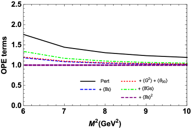
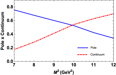
Figure 1: The OPE convergence of the sum rules: The ratio of the sum of the contributions up to specified dimension to the total contribution is plotted with respect to  $M^{2}$ at $s_{0}=134~{}\mathrm{GeV^{2}},T=0$  (left). Pole dominance of the sum rules: relative contributions of the pole (blue) and continuum (red-dashed) versus the Borel parameter $M^{2}$ at $s_{0}=134~{}\mathrm{GeV^{2}},T=0$ (right).

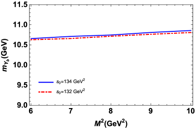
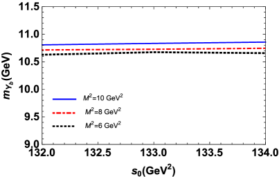
Figure 2: Mass of $Y_{b}$ as a function of $M^{2}$ (left) and $s_{0}$ (right).

Table 2: Results obtained in this work for the mass of $Y_{b}$ at $T=0$, in comparison with literature.

	$m_{Y_{b}}(\mathrm{MeV})$
Present Work	$10735^{+122}_{-107}$
Experiment	$10889.9^{+3.2}_{-2.6}$ [31]
QCDSR	$10880\pm 130$ [11]
	$10910\pm 70$ [10]

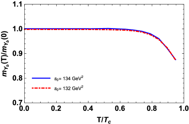
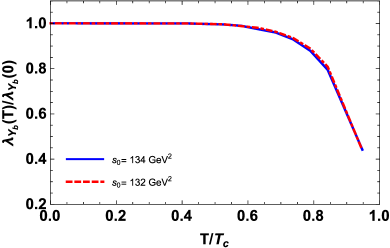
Figure 3: The mass (left) and pole residue (right) of $Y_{b}$ as a function of temperature.

After testing the sum rules at $T=0$, and comparing the obtained results, the temperature dependence of the mass and the pole residue of $Y_{b}$ is plotted in Figure 3. Thermal behavior of mass and pole residue of $Y_{b}$ are monotonous until $T\cong 0.12~{}\mathrm{\mathrm{GeV}}$. However, after this point, they begin to decrease promptly with increasing temperature. At the vicinity of the critical (or so called deconfinement) temperature, the mass reaches nearly $87\%$ of its vacuum value. On the other hand, the pole residue is decreased to $44\%$ of its value at vacuum. Even though the thermal dependencies indicate that the mass and the pole residue of $Y_{b}$ might dissolve at $T_{c}$, its temperature dependent decay behavior should also be studied to conclude on the stability of the state. Since the decay properties also depend on temperature, and while the mass and pole residue diminish, the decay width might increase with increasing temperature [43], decay widths at finite temperature should also be investigated. However the current status of $Y_{b}$ resonance is very complicated, since it is very close to $\Upsilon(5S)$. Thus studying its decays requires establishment of a good model in the hidden-beauty sector.

4 Concluding Remarks

In this work, we revisited the hidden beauty exotic state $Y_{b}$, and studied its properties at vacuum and finite temperatures. To describe the hot medium effects to the hadronic parameters of the resonance $Y_{b}$, TQCDSR method is used considering contributions of condensates up to dimension six. Our results are in reasonable agreement with the available experimental data and other vacuum QCD sum rules works in the literature. Numerical findings show that $Y_{b}$ can be well described by a scalar-vector tetraquark current. In addition, we observed that until temperature $T\simeq 120~{}\mathrm{MeV}$ the mass and pole residue values stay nearly same with QCD vacuum values. However after this point increasing temperature behaviors of the mass and the pole residue is changed remarkably, and they reduced approximately to $87\%$ and $44\%$ of their vacuum values, respectively. These findings are in good agreement with the temperature behavior of conventional hadrons, and also with exotic states. In the literature, remarkable drop in the values of the mass and the pole residue in hot medium was regarded as the signal of the QGP, which is called as the fifth state of matter, phase transition. Also, studying of $Y_{b}$ state in hot medium can be a useful tool to analyze results of the heavy-ion collision experiments. We hope that precise spectroscopic measurements in the exotic bottomonium sector can be done at Super-B factories, and this might provide conclusive answers on the nature and thermal behaviors of the exotic states.

Appendix A Thermal spectral density $\rho^{\mathrm{QCD}}(s,T)$ for $Y_{b}$ state

In this appendix, the explicit forms of the spectral densities obtained in this work are presented. The expressions for $\rho^{\mathrm{pert.}}(s)$ and $\rho^{\mathrm{nonpert.}}(s,T)$ are shown below as integrals over the Feynman parameters $z$ and $w$, where $\theta$ is the step function,

$$\rho^{\mathrm{pert.}}(s) = \frac{1}{3072\pi^{6}}\int_{0}^{1}dz\int_{0}^{1-z}dw$$ (25)

$$\times \frac{1}{\kappa^{8}\xi^{2}}\Bigg{\{}\Big{[}-\kappa m_{b}^{2}(z+w)+szw\xi\Big{]}^{2}\Big{[}\kappa^{2}m_{b}^{4}zw(z+w)[w^{2}+(-1+w)$$

$$\times w+z(-1+4w)]-2\kappa m_{b}^{2}\Big{[}6m_{s}^{2}\Phi^{2}[7(-1+z)z(-7+8z)$$

$$\times w+7w^{2}]+sz^{2}w^{2}(12(-1+z)z+(-12+25z)w$$

$$+ 12w^{2})\Big{]}\xi+szw(12m_{s}^{2}\Phi^{2}+35sz^{2}w^{2})\xi^{3}\Big{]}\Bigg{\}}~{}\theta[L(s,w,z)],$$

$$\rho^{\langle s\bar{s}\rangle}(s,T) = \frac{\langle\bar{s}s\rangle}{128\pi^{4}}\int_{0}^{1}dz\int_{0}^{1-z}dw\frac{1}{\kappa^{6}}\Bigg{\{}\Big{[}\kappa^{3}m_{b}^{5}w(z+w)^{2}+\kappa^{2}m_{b}^{4}m_{s}(z+w)$$ (26)

$$\times [19z^{4}+19(-1+w)^{2}w^{2}+2z(-1+w)w(-19+25w)+z^{3}$$

$$\times (-38+50w)+z^{2}[19+w(-88+81w)]\Big{]}-\kappa^{2}m_{b}^{3}z(z+w)$$

$$\times (m_{s}^{2}\Phi+2sw^{2})\xi-\kappa m_{b}^{2}m_{s}szw\Big{[}22z^{4}+22(-1+w)^{2}w^{2}+z^{3}$$

$$\times (-44+111w)+z(-1+w)w(-44+111w)+z^{2}[22+w$$

$$\times (-155+197w)]\Big{]}\xi+\kappa m_{b}sz^{2}w(m_{s}^{2}\Phi+sw^{2})\xi^{2}+3m_{s}s^{2}z^{2}$$

$$\times w^{2}\Big{(}z^{2}+(-1+w)w+z(-1+21w)\Big{)}\xi^{3}\Big{]}\Bigg{\}}~{}\theta[L(s,w,z)],$$

$$\rho^{\langle G^{2}\rangle+\langle\Theta_{00}\rangle}(s,T) = \frac{1}{4608\pi^{2}}\int_{0}^{1}dz\int_{0}^{1-z}dw$$ (27)

$$\times \frac{1}{\kappa^{6}\xi^{2}}\Bigg{\{}192\pi^{2}\langle\Theta^{f}_{00}\rangle zw\xi^{2}\Bigg{[}m_{b}^{4}\Phi^{2}(z+w)[3(-1+z)z+(-3+5z)$$

$$\times w+3w^{2}]+m_{b}^{2}\Phi szw[-27(-1+z)z+27w-53zw-27w^{2}]$$

$$\times \xi+30s^{2}z^{2}w^{2}\xi^{3}\Bigg{]}-g_{s}^{2}\langle\Theta^{g}_{00}\rangle\Big{[}3m_{b}^{4}\Phi^{2}zw(z+w)[2(-1+z)^{2}z^{2}$$

$$+ (-1+z)z(-4+3z)w+(-2+z)(-1+3z)w^{2}+(-4+3z)$$

$$\times w^{3}+2w^{4}]-m_{b}^{2}\Phi sz^{2}w^{2}[24(-1+z)^{2}z^{2}+(-1+z)z(-48+85$$

$$\times z)w+[24+z(-133+121z)]w^{2}+(-48+85z)w^{3}+24w^{4}]\xi$$

$$- 12m_{b}^{3}m_{s}\Phi^{3}(z+w)^{3}\xi^{2}+12m_{b}m_{s}\Phi^{2}szz(z^{2}+10zw+w^{2})\xi^{3}+30$$

$$\times s^{2}z^{3}w^{3}(z+w)\xi^{4}\Big{]}+\langle\frac{\alpha_{s}G^{2}}{\pi}\rangle\pi^{2}\Bigg{[}\kappa m_{b}^{2}\Big{\{}-6m_{s}^{2}\Phi^{2}\big{[}5(-1+z)z^{3}+z^{3}$$

$$\times w+(-5+z)w^{3}+5w^{4}\big{]}+sz^{2}w^{2}[2(-1+z)z^{2}(-18+11z)+z$$

$$\times [72+z(-221+133z)]w+[36+z(-221+231z)]w^{2}(-58+133$$

$$\times z)w^{3}+22w^{4}]\Big{\}}\xi-36\kappa^{3}m_{b}^{3}m_{s}(z+w)(z^{2}-6zw+w^{2})\xi^{2}-60s^{2}$$

$$\times z^{3}w^{3}(z+w)\xi^{4}+\xi^{2}m_{b}zw[m_{b}^{3}(z+w)(4(-1+z)z^{2}(-3+4z)$$

$$+ 6z[4+z(-11+8z)]w+[12+11z(-6+5z)]w^{2}4(-7+12z)$$

$$\times w^{3}+16w^{4})+12m_{s}s(3z^{2}-26zw+3w^{2})\xi^{3}]\Bigg{]}\Bigg{\}}~{}\theta[L(s,w,z)]$$

$$\rho^{\langle\bar{s}Gs\rangle}(s,T) = \frac{m_{s}m_{0}^{2}\langle\overline{s}s\rangle}{64\pi^{4}}\Bigg{\{}\int_{0}^{1}dz\Big{\{}3m_{b}^{2}+s(z-1)z~{}\theta[L^{\prime}(s,z)]\Big{\}}$$ (28)

$$+ \int_{0}^{1}dz\int_{0}^{1-z}dw\frac{1}{3\kappa^{5}}\Big{\{}zw\xi\Big{[}\kappa m_{b}^{2}[5z^{2}+5(w-1)w+z(11w-5)]$$

$$- 16szw\xi^{2}\Big{]}~{}\theta[L(s,w,z)]\Big{\}}\Bigg{\}},$$

$$\rho^{\langle\overline{s}s\rangle^{2}}(s,T) = \frac{\langle\overline{s}s\rangle^{2}}{5184\pi^{4}}\Bigg{\{}\int_{0}^{1}dz\Big{[}648m_{b}^{2}\pi^{2}+g_{s}^{2}m_{b}m_{s}z+54\pi^{2}(5m_{s}^{2}+4s)(z-1)z\Big{]}$$ (29)

$$\times \theta[L^{\prime}(s,z)]+g_{s}^{2}\int_{0}^{1}dz\int_{0}^{1-z}\frac{dwzw\xi}{\kappa^{5}}\Big{[}3\kappa m_{b}^{2}[7z^{2}+7(w-1)w$$

$$+ z(-7+15w)]-64szw\xi^{2}\Big{]}~{}\theta[L(s,w,z)]\Bigg{\}},$$

where explicit expressions of the functions $L(s,w,z)$ and $L^{\prime}(s,z)$ are

$$L[(s,w,z) = \frac{(-1+w)\Big{[}(-1+w)w^{2}+2(-1+w)wz+(-1+2w)z^{2}-swz\xi+z^{3}m_{b}^{2}\Big{]}}{\kappa^{2}},$$

$$L^{\prime}(s,z) = sz(1-z)-m_{b}^{2}.$$ (30)

The below definitions are used for simplicity:

$$\kappa = z^{2}+z(w-1)+(w-1)w,$$

$$\Phi = (z-1)w+(z-1)w+w^{2},$$

$$\xi = z+w-1.$$ (31)

References

References

- [1] Segovia J, Ortega P G, Entem D R and Fern ndez F 2016 Phys. Rev. D 93, 7, 074027
- [2] Chen K F et al. [Belle Collaboration] 2008 Phys. Rev. Lett. 100, 112001
- [3] Aubert B et al. [BaBar Collaboration] 2009 Phys. Rev. Lett. 102, 012001
- [4] Huang G S et al. [CLEO Collaboration] 2007 Phys. Rev. D 75, 012002
- [5] Chen K F et al. [Belle Collaboration] 2010 Phys. Rev. D 82, 091106
- [6] Bonvicini G et al. [CLEO Collaboration] 2006 Phys. Rev. Lett. 96, 022002
- [7] Jaffe R L 1977 Phys. Rev. Lett. 38, 195
- [8] Maiani L, Piccinini F, Polosa A D and Riquer V 2005 Phys. Rev. D 71, 014028
- [9] Chen Y D and Qiao C F 2012 Phys. Rev. D 85, 034034
- [10] Albuquerque R M, Nielsen M and da Silva R R 2011 Phys. Rev. D 84, 116004
- [11] Zhang J R and Huang M Q 2010 JHEP 1011, 057
- [12] Chatrchyan S et al. [CMS Collaboration] 2012 Phys. Rev. Lett. 109, 222301 Erratum: [Phys. Rev. Lett. 120, 19, 199903 (2018)]
- [13] Sirunyan A M et al. [CMS Collaboration] 2017 Phys. Rev. Lett. 118, 16, 162301
- [14] Sirunyan A M et al. [CMS Collaboration] 2018 Phys. Rev. Lett. 120, 14, 142301
- [15] Sirunyan A M et al. [CMS Collaboration], arXiv:1805.09215 [hep-ex].
- [16] Mocsy A and Petreczky P 2007 Phys. Rev. Lett. 99, 211602
- [17] Burnier Y, Kaczmarek O and Rothkopf A 2015 JHEP 1512, 101
- [18] Shifman M A, Vainshtein A I and Zakharov V I 1979 Nucl. Phys. B 147, 385
- [19] Reinders L J, Rubinstein H and Yazaki S 1985 Phys. Rept. 127, 1
- [20] Colangelo P and Khodjamirian A 2000 Shifman, M. (ed.): At the Frontier of Particle Physics 3, 1495
- [21] Narison S 2002 Camb. Monogr. Part. Phys. Nucl. Phys. Cosmol. 17, 1
- [22] Bochkarev A I and Shaposhnikov M E 1986 Nucl. Phys. B 268, 220
- [23] Hatsuda T, Koike Y and Lee S H 1993 Nucl. Phys. B 394, 221
- [24] Alam J, Sarkar S, Roy P, Hatsuda T and Sinha B 2001 Annals Phys. 286, 159
- [25] Rapp R, Wambach J and Hees H van 2010 Landolt-Bornstein 23, 134
- [26] Mallik S and Mukherjee K 1998 Phys. Rev. D 58, 096011
- [27] Dominguez C A, Loewe M and Zhang Y 2013 Phys. Rev. D 88, 054015
- [28] Veliev E V, Günaydın S and Sundu H 2018 EPJ Plus 133, 139
- [29] Matheus R D, Narison S, Nielsen M and Richard J M 2007 Phys. Rev. D 75, 014005
- [30] Mallik S 1998 Phys. Lett. B 416, 373
- [31] Tanabashi M et al. (Particle Data Group) 2018 Phys. Rev. D 98, 030001
- [32] Dosch H G, Jamin M and Narison S 1989 Phys. Lett. B 220, 251
- [33] Belyaev V M and Ioffe B L 1983 Sov. Phys. JETP 57, 716 [Zh. Eksp. Teor. Fiz. 84, 1236]
- [34] Ioffe B L 2006 Prog. Part. Nucl. Phys. 56, 232
- [35] Azizi K and Bozkır G 2016 Eur. Phys. J. C 76, 10, 521
- [36] Ayala A, Bashir A, Dominguez C A, Gutierrez E, Loewe M and Raya A 2011 Phys. Rev. D 84, 056004
- [37] Bazavov A et al. 2009 Phys. Rev. D 80, 014504
- [38] Cheng A et al. 2010 Phys. Rev. D 81, 054504
- [39] Ayala A, Dominguez C A, Loewe M, Zhang Y 2012 Phys. Rev. D 86, 114036
- [40] Cheng M et al. 2008 Phys. Rev. D 77, 014511
- [41] Dominguez C A, Loewe M, Rojas J C and Zhang Y 2010 Phys. Rev. D 81, 014007
- [42] Veliev E V, Sundu H, Azizi K and Bayar M 2010 Phys. Rev. D 82, 056012
- [43] Azizi K and Er N 2010 Phys. Rev. D 81, 096001