Fickian and non-Fickian diffusion of cosmic rays

Abstract

Fluid approximations to cosmic ray (CR) transport are often preferred to kinetic descriptions in studies of the dynamics of the interstellar medium (ISM) of galaxies, because they allow simpler analytical and numerical treatments. Magnetohydrodynamic (MHD) simulations of the ISM usually incorporate CR dynamics as an advection-diffusion equation for CR energy density, with anisotropic, magnetic field-aligned diffusion with the diffusive flux assumed to obey Fick’s law. We compare test-particle and fluid simulations of CRs in a random magnetic field. We demonstrate that a non-Fickian prescription of CR diffusion, which corresponds to the telegraph equation for the CR energy density, can be easily calibrated to match the test particle simulations with great accuracy. In particular, we consider a random magnetic field in the fluid simulation that has a lower spatial resolution than that used in the particle simulation to demonstrate that an appropriate choice of the diffusion tensor can account effectively for the unresolved (subgrid) scales of the magnetic field. We show that the characteristic time which appears in the telegraph equation can be physically interpreted as the time required for the particles to reach a diffusive regime and we stress that the Fickian description of the CR fluid is unable to describe complex boundary or initial conditions for the CR energy flux.

1 Introduction

Cosmic rays (CRs) are an important ingredient of the interstellar medium (ISM) of galaxies, with a typical energy density comparable to the magnetic energy density and the turbulent gas kinetic energy density, and they contribute significantly to the support of the galactic gaseous discs against gravity and drive galactic outflows (Kulsrud, 2005). Significant efforts have been made to include CRs in MHD simulations of the ISM and assess their importance in the outflows (e.g., Simpson et al., 2016; Girichidis et al., 2016; Holguin et al., 2018; Farber et al., 2018) and galactic dynamos (e.g., Hanasz et al., 2009). The transport of CRs is usually quite simplified in these works, where the CR population is modelled as a single fluid under the advection-diffusion approximation, with the diffusive flux taken to follow Fick’s law. CR diffusion is assumed to be either isotropic, anisotropic but with negligible diffusion perpendicular to the magnetic field, or to have both parallel and perpendicular diffusivities (Strong et al., 2007; Zweibel, 2013; Grenier et al., 2015; Zweibel, 2017). In all of these cases, constant values are taken for the diffusivities, with a parallel (or isotropic) component typically of order $\kappa_{\parallel}=10^{28}\,{\rm cm}^{2}\,{\rm s}^{-1}$ and a perpendicular diffusivity, $\kappa_{\perp}$, $10\text{--}1000$ times smaller.

Meanwhile, a coherent theory of CR propagation and confinement has been sought, mostly using quasi-linear theory (see Strong et al., 2007, and references therein) verified and extended using simulations of test particles (e.g., Snodin et al., 2016, and references therein).

One of the dynamical roles of CRs in the ISM is to provide an additional force due to their pressure gradient that acts on the background gas. The CR particles responsible for this effect gyrate about magnetic field lines with a Larmor radius that is much smaller than scales resolved in modern ISM simulations. The CR fluid description should then account for the effective CR dynamics at the scale resolved in the simulations. Here we consider CR diffusion in random magnetic fields which can be examined via test-particle simulations where the relevant small scales are reasonably well resolved. We devise simple numerical experiments to examine whether anisotropic diffusion prescriptions with constant $\kappa_{\parallel}/\kappa_{\perp}$, applied to fluid simulations at a relatively low spatial resolution can capture the properties of test particle propagation in simulations at higher resolution. In particular, we compare the standard anisotropic Fickian diffusion of CRs with a non-Fickian one that leads, instead of the diffusion equation, to the telegraph equation for the number (or energy) density of the particles. The telegraph equation contains an additional time scale $\tau$ which accounts for the finite propagation speed of the CR distribution (e.g., Bakunin, 2008) and allows for the differentiation between the early ballistic behaviour of the particles and the subsequent diffusive CR spread. The telegraph equation is also a convenient way to avoid numerical problems close to singular magnetic X-points, and may also allow for larger time steps in an explicit numerical scheme than that with the Fickian approach (Snodin et al., 2006). Litvinenko & Noble (2016) compare numerical solutions of fluid equations for cosmic ray propagation that result from various approximations to the Fokker–Planck equation, including the telegraph equation, and confirm the relevance of this approximation. Our goal is to compare test-particle simulations of cosmic ray propagation with the telegraph-equation approximation to derive optimal parameters of the latter that can inform sub-grid models of cosmic ray propagation in a comprehensive MHD simulation of the multi-phase interstellar medium. We discuss the dependence of the CR diffusion parameters on the CR properties, on the test particle magnetic field power spectrum and on the resolution of the fluid simulation. We describe our numerical experiments with test particle and fluid descriptions in Sections 2.1 and 2.2, respectively. The general results and a proposed calibration procedure for the diffusion parameters are presented in Sections 3.1 and 3.2. In Section 4, we discuss the results further and summarise our conclusions.

2 Numerical experiments

2.1 Test particle simulations

We use test particle simulations of CR propagation in a random magnetic field as a reference to which fluid simulations can be compared and calibrated. These simulations are very similar to those performed by Snodin et al. (2016). For a direct comparison with fluid simulations, we construct a random, time-independent, periodic, magnetic field $\bm{B}(\bm{x})$ on a uniform Cartesian mesh of side length $L$ and resolution $1280$ points in each direction (the discrete model described by Snodin et al., 2016). We use an isotropic magnetic field with a power spectrum $M(k)\propto k^{s}$, over the range $k_{\text{min}}\leq k\leq k_{\text{max}}^{\text{particle}}$, with $k_{\text{min}}=2{\rm\pi}/L$ and $k_{\text{max}}^{\text{particle}}=640{\rm\pi}/L=320k_{\text{min}}$, and consider the cases $s=-5/3$, and $s=-2$. Within the simulation volume $L^{3}$, we placed $2.1\times 10^{7}$ test particles of a given energy, initially distributed in space so that their number density follows

$$n(x,y,z)\propto\exp\left[-\frac{x^{2}}{2\sigma_{0}^{2}}\right],\quad(x,y,z)\in[-L/2,L/2]^{3}\,,$$ (1)

being non-uniform in the $x$-direction but homogeneous in the other directions. The half-width $\sigma_{0}$ was chosen to correspond to approximately 71 mesh points ($0.0552L$). The initial velocities of the particles were distributed isotropically. For each particle, we then solved the equation of motion

$$\ddot{\bm{x}}=\alpha\dot{\bm{x}}\times\bm{B}[\bm{x}(t)]\,,$$ (2)

where $\bm{x}(t)$ is the particle position, $\alpha=qLB_{\mathrm{rms}}/(\gamma mcv_{0})$, with $q$ the particle charge, $m$ the particle mass, $\gamma$ the particle Lorentz factor, $c$ the speed of light, $v_{0}$ a reference speed, and $B_{\mathrm{rms}}$ the root-mean-square magnetic field strength. Here we neglect electric fields, so that the particle energy is conserved. We take $\alpha=320$, and $v/v_{0}=1$ for each particle, so that the dimensionless Larmor radius, $R_{\rm L}/L=1/320$, is somewhat smaller than the scales resolved in the fluid simulations discussed below, but also a few times larger than the test-particle grid resolution. Typically, each particle trajectory was integrated up to a maximum dimensionless time of $t=2.8$, corresponding to approximately $142t_{\rm L}$, where $t_{\rm L}=2\pi R_{\rm L}/v_{0}$ is the Larmor time scale.

2.2 Fluid description of CR propagation

We compare the test-particle results with simulations where the CRs are approximated as a fluid governed by the equations (Snodin et al., 2006)

$$\frac{\partial\varepsilon}{\partial t}=-\nabla\cdot\bm{{F}}\,\;,\qquad\tau\frac{\partial{F}_{i}}{\partial t}=-\kappa_{ij}\nabla_{j}\varepsilon-{F}_{i}\,,$$ (3)

where $\varepsilon$ is the CR energy density, $\bm{{F}}$ is the associated energy flux and $\kappa_{ij}$ is a diffusion tensor given by

$$\kappa_{ij}=\kappa_{\perp}\delta_{ij}+(\kappa_{\parallel}-\kappa_{\perp})\hat{B}_{i}\hat{B}_{j}\,,$$ (4)

where $\hat{\bm{B}}=\bm{B}/|\bm{B}|$ is the unit vector along the magnetic field. Here the diffusivity along magnetic field lines is usually taken to be much larger than the diffusivity perpendicular to field lines, $\kappa_{\parallel}\gg\kappa_{\perp}$. The case $\tau=0$ corresponds to anisotropic Fickian diffusion, which we refer to as the Fickian prescription. The case $\tau=0$ leads to the CR distribution spreading at an infinite speed, so that an initially spatially localised CR energy distribution will be redistributed over all space available after any finite time. This is a well-known artefact of the diffusion approximation. When $\tau\neq 0$, these equations correspond to a generalised form of the telegraph equation for $\varepsilon$, which we shall refer to as the Telegraph prescription.

2.2.1 CR propagation and the telegraph equation

The telegraph equation for the CR distribution function has been studied in several previous works (e.g., Gombosi et al., 1993; Litvinenko & Schlickeiser, 2013; Tautz & Lerche, 2016), including its connection to a hyperdiffusive equation that arises more naturally in higher-order expansions of the energy flux (Malkov & Sagdeev, 2015). The main reason for using this prescription has been to capture the non-diffusive behaviour at short times, corresponding to (superdiffusive) ballistic particle motion, followed by a transition to the diffusive regime. For the CR distribution function, the time scale $\tau$ can be connected with the pitch angle diffusivity (Litvinenko & Schlickeiser, 2013). One difference from the Fickian case is that the maximum signal propagation speed (parallel to magnetic field lines) is reduced to $(\kappa_{\parallel}/\tau)^{1/2}$.

It has been claimed that the telegraph equation is not suitable for modelling CR propagation as it does not conserve the total number of particles or, equivalently, their total energy (Malkov & Sagdeev, 2015); see also Tautz & Lerche (2016). However, this assertion seems to be based on misunderstanding. Indeed, consider the one-dimensional telegraph equation for the energy density of particles $\varepsilon(x,t)$ in $|x|<\infty$:

$$\tau\frac{\partial^{2}\varepsilon}{\partial t^{2}}+\frac{\partial\varepsilon}{\partial t}+V\frac{\partial\varepsilon}{\partial x}=\kappa\frac{\partial^{2}\varepsilon}{\partial x^{2}}\,,$$ (5)

where $V$ is the advection speed, assumed to be constant for simplicity, and $\kappa$ is the diffusivity. Adopting natural boundary conditions $\varepsilon=0$ and $\partial\varepsilon/\partial x=0$ at $x=\pm\infty$, the total energy of the particles $E(t)=\int_{-\infty}^{\infty}\varepsilon(x,t)\,\mathrm{d}x$ can easily be shown to satisfy

$$\frac{\mathrm{d}E}{\mathrm{d}t}+\tau\frac{\mathrm{d}^{2}E}{\mathrm{d}t^{2}}=0\,,$$ (6)

which solves to yield

$$E=C+K\mathrm{e}^{-t/\tau}\,,$$ (7)

where $C$ and $K$ are constants. Since the telegraph equation is of second order in $t$, two initial conditions for $E(t)$ have to be specified: $E(0)=E_{0}$ at $t=0$ for the initial energy and $\partial E/\partial t=0$ at $t=0$. Then the only admissible solution is $E=E_{0}=\mathrm{const}$, expressing the conservation of the total energy (and similarly for the total number of particles). Other authors disregard the second initial condition, which seems to be the cause of confusion regarding the conservation of $E$, as they then analyse an incomplete solution $E=E_{0}+K(\mathrm{e}^{-t/\tau}-1)$.

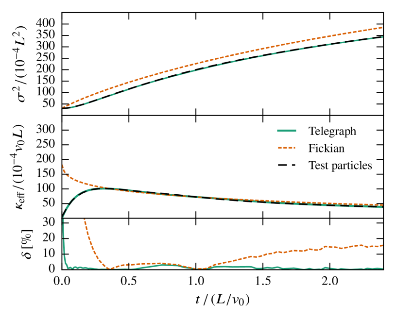
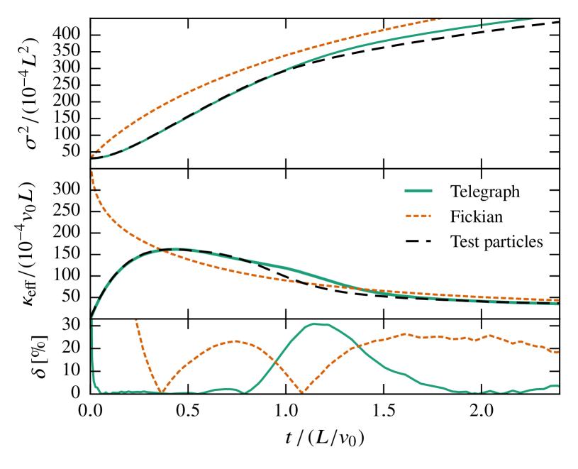
Figure 1: Comparison between the results of test particle simulations and fluid simulations using the Telegraph and Fickian prescriptions (with the same choice of calibrated diffusivities $\kappa_{\parallel}$ and $\kappa_{\perp}$) for a magnetic field with $s=-5/3$, in the left-hand side column, and $s=-2$ on the right. The top panels show time evolution of the variance $\sigma^{2}$ of the CR distribution along the $x$-axis, the middle panels show the time evolution of the effective diffusivity, $\kappa_{\text{eff}}=\tfrac{1}{2}\partial\sigma^{2}/\partial t$, and bottom panels show the relative difference in $\kappa_{\text{eff}}$, $\delta=(\kappa_{\text{eff},\text{f}}-\kappa_{\text{eff},\text{p}})/\kappa_{\text{eff},\text{p}}$, with indices ‘f’ and ‘p’ referring to the fluid and test particle descriptions.

2.2.2 Fluid simulations

We solve equations (3) and (4) using the Pencil Code (Brandenburg & Dobler, 2010), a code for non-ideal MHD using sixth-order spatial finite differences. The simulation domain comprises a box of $80^{3}$ grid points, with periodic boundary conditions. The magnetic field is the same as that used in the test particle simulation, but with the smallest scales removed by truncating the spectrum $M(k)$ at $k_{\text{max}}^{\text{fluid}}=40\pi/L=k_{\text{max}}^{\text{particle}}/16$, resulting in a magnetic field specified on a coarser grid. As in the test-particle simulations, the magnetic field does not evolve during the simulation.

The choice of a much coarser resolution for the magnetic field in the fluid simulation reflects the fact that it is usually not feasible to simultaneously resolve the scales of interest of a particular astrophysical problem and the Larmor radius of the relevant CR population. For example, the typical resolution in simulations of milti-phase supernova-driven ISM is of order of a few $\,{\rm pc}$, while the Larmor radius is of order $10^{-6}$–$10^{-5}\,{\rm pc}$ for cosmic ray energies of $1\text{--}10\,{\rm GeV}$ in a $5\,\mu{\rm G}$ magnetic field. Thus, any effects arising from the unresolved small scales, $k>k_{\text{max}}^{\text{fluid}}$, need to be accounted for through an adequate choice of the parameters that control CR diffusion, i.e., the diffusivities $\kappa_{\parallel}$, $\kappa_{\perp}$, and, in the Telegraph case, the characteristic timescale $\tau$.

We chose an initial condition for the CR energy density consistent with the particle distribution in Eq. (1) by assuming a single population of CRs, i.e., $\varepsilon(x,y,z)=n(x,y,z)E{{}_{\mathrm{cr}}}$, where $n$ is the particle number density and $E{{}_{\mathrm{cr}}}$ is the energy of an individual particle. In the fluid simulation, the initial half-width of the CR distribution, $\sigma_{0}$, corresponds to approximately $4.4$ mesh points, consistent with the particle simulations.

While in the Fickian prescription the initial condition for $\bm{{F}}$ is fully determined by the initial condition for $\varepsilon$, the Telegraph prescription requires a separate initial condition for $\bm{{F}}$. In agreement with the initial condition used for the particles, whose initial velocities have random, isotropic directions, we impose the zero flux initial condition, $\bm{{F}}=\bm{0}$.

3 Results

3.1 Test particle simulations

Results of the test particle simulations are shown as dashed curves in Fig. 1, where the magnetic field has spectral index $s=-5/3$ (left-hand column) and $s=-2$ (right-hand column). In the upper panels, we show the variance $\sigma^{2}$ of the CR number density distribution along the $x$-axis as a function of time. The global effective diffusivity $\kappa_{\text{eff}}\equiv\frac{1}{2}\operatorname*{d\!}\sigma^{2}/\operatorname*{d\!}t$ is shown in the middle panels. The variance $\sigma^{2}$ of the test particle distribution deviates strongly from the simple linear dependence on time that would be expected in the case of an isotropic Fickian diffusion. This is also visible in the variation of $\kappa_{\text{eff}}$ with time, which first increases sharply, reaches a peak, and then decays to an asymptotic value. This behaviour reflects the transition from ballistic to diffusive behaviour and is characterised by the time interval $t_{\text{peak}}$ after which $\kappa_{\text{eff}}$ reaches a maximum $\kappa_{\text{peak}}$. The transition is sensitive to the spectral index of the random field, with $t_{\text{peak}}\approx 0.31L/v_{0}$ for $s=-5/3$ and $t_{\text{peak}}\approx 0.43L/v_{0}$ for $s=-2$.

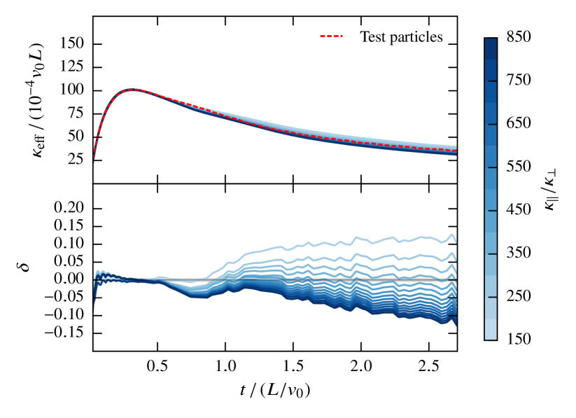
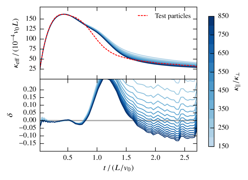
Figure 2: Impact of the choice of the ratio $r=\kappa_{\parallel}/\kappa_{\perp}$ for a magnetic field with $s=-5/3$ (left-hand column), and $s=-2$ (right-hand column). The top panels show the time evolution of the effective global diffusivity $\kappa_{\text{eff}}$ for properly calibrated Telegraph models with different choices of $r$ (colour-coded, with the colour bar shown oon the right of each column). The bottom panels show the fractional error in $\kappa_{\text{eff}}$.

3.2 Fluid simulations

We found that it is possible to reproduce the behaviour of the test particle simulation with the Telegraph fluid simulation. For a fixed value of $r=\kappa_{\parallel}/\kappa_{\perp}$, we found that $t_{\text{peak}}$ and $\kappa_{\text{peak}}$ are controlled by $\tau$ and $\kappa_{\parallel}$, respectively. Therefore, the fluid simulation can be calibrated using the following simple iterative procedure, where the iteration steps are labelled with index $i$:

$$\kappa_{\parallel}^{(i+1)}=\kappa_{\parallel}^{(i)}\left.\frac{\kappa_{\text{peak}}^{\text{particle}}}{\kappa_{\text{peak}}^{(i)}}\right.\;,\quad\tau^{(i+1)}=\tau^{(i)}\left.\frac{t_{\text{peak}}^{\text{particle}}}{t_{\text{peak}}^{(i)}}\right.\,.$$ (8)

Thus, one runs a fluid simulation for given $\kappa_{\parallel}^{(i)}$ and $\tau^{(i)}$, and from this run $\kappa_{\text{peak}}^{(i)}$ and $t_{\text{peak}}^{(i)}$ are computed. Then, in the next iteration, the fluid simulation is re-run using $\kappa_{\parallel}^{(i+1)}$ and $\tau^{(i+1)}$; note that for this particular simulation setup the computational cost of each run is very low. The iteration is performed until both $\kappa_{\text{peak}}$ and $t_{\text{peak}}$ differ from $\kappa_{\text{peak}}^{\text{particle}}$ and $t_{\text{peak}}^{\text{particle}}$, respectively, by less than $0.5$ per cent. The iterations typically converge to this accuracy in 2–4 steps.

In Fig. 2, each of the curves is obtained with a different choice of $r$, calibrated using Eq. (8). This ratio controls the slope of $\kappa_{\text{eff}}(t)$ at late times, therefore controlling the asymptotic value of $\kappa_{\text{eff}}$. The relative difference between $\kappa_{\text{eff}}$ obtained from the fluid and particle simulations, $\delta=(\kappa_{\text{eff}}^{\text{fluid}}-\kappa_{\text{eff}}^{\text{particle}})/\kappa_{\text{eff}}^{\text{particle}}$, is shown in the bottom panel. We use the time averaged value $\langle\delta\rangle$ as a goodness-of-fit measure, which is shown in Fig. 3. We find that the ratio $r=\kappa_{\parallel}/\kappa_{\perp}$ giving the best fit to the test-particle results depends on the spectrum of the magnetic field, with $r\approx 325$ for $s=-5/3$, and $r\approx 525$ for $s=-2$.

Table 1: The best-fit parameters used in th fluid simulations shown in Fig. 1, values of $t_{\text{peak}}$ and $\kappa_{\text{peak}}$, and their relation to the model parameters.

	$s=-5/3$	$s=-2$
$\kappa_{\text{peak}}/(v_{0}L)$	0.010	0.016
$\kappa_{\parallel}/(v_{0}L)$	0.054	0.109
$\kappa_{\perp}/(v_{0}L)$	0.00017	0.00021
$\kappa_{\parallel}/\kappa_{\perp}$	325	525
$t_{\text{peak}}/(L/v_{0})$	0.31	0.43
$\tau/(L/v_{0})$	0.17	0.33
$\kappa_{\parallel}/\kappa_{\text{peak}}$	5.35	6.70
$\tau/t_{\text{peak}}$	0.55	0.77
$(\kappa_{\parallel}/\tau)^{1/2}/v_{0}$	0.56	0.57

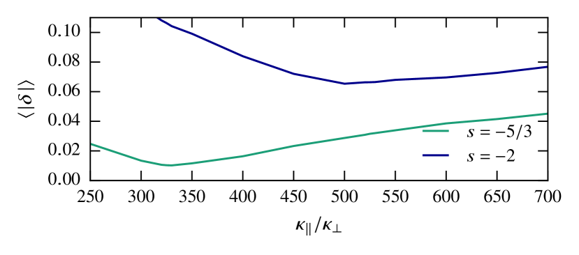
Figure 3: The time-averaged fractional error in $\kappa_{\text{eff}}$ as a function of the ratio of CR diffusivities for two choices of the spectral index of the magnetic spectrum as specified in the legend.

The best fit parameters are summarised in Table 1 and correspond to the solid green curves in Fig. 1. The dashed orange curves in those figures show the Fickian prescription for the same choice of $\kappa_{\parallel}$ and $\kappa_{\perp}$. The lower panels of those figures show $\delta$ for both fluid prescriptions compared with the test particle simulation. For $s=-5/3$, the effective diffusivity, $\kappa_{\text{eff}}$ of the CR distribution resulting from the calibrated Telegraph simulation differs from that in the test particle simulation by at most $2$ per cent at any time. For $s=-2$ we find similarly small differences in $\kappa_{\text{eff}}$ for $t\lesssim 0.8L/v_{0}$ and $t\gtrsim 1.7L/v_{0}$, but $\delta$ increases up to $\sim 30$ per cent for $t\approx 1.1L/v_{0}$. This leaves an imprint in the variance at later times (top right panel of Fig. 1). Albeit small, such a feature occurs independent of the specific parameter choice (see right panel of Fig. 2). The Fickian solution does not capture the ballistic phase of particle propagation. However, at sufficiently large times, the effective diffusivity in the Fickian case is in good agreement with both the Telegraph and test particle results. In considering these differences, it is perhaps worth noting that the diffusion coefficient is typically unknown by almost a factor of two.

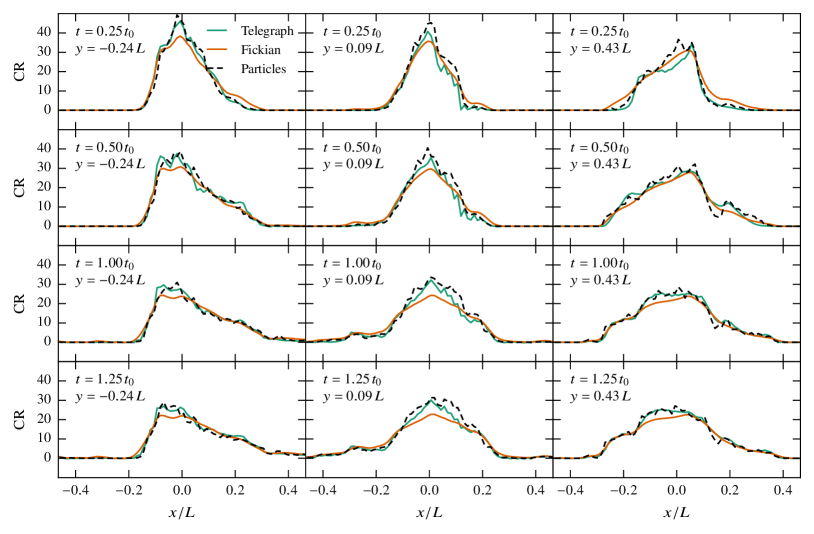
Figure 4: Time evolution (top to bottom) of the CR distribution along the $x$-axis obtained by integrating the results over parallelepipeds extended along the $x$-axis and $0.05L$ in width along $y$ and $z$ passing through arbitrarily chosen positions in $y$ and $z$ (left to right). The vertical axis shows, in arbitrary units, the total number of particles and their energy in the integration domain. The higher accuracy of the Telegraph model is apparent.

The calibrated Telegraph model is able to reproduce local features, as shown in Fig. 4, where slices through the test particle simulation box are compared with the corresponding slices of the fluid simulations at various times and locations. Both the asymmetry in the distribution and small-scale variations are reproduced better by the Telegraph model.

3.3 Variability of $t_{\text{peak}}$ in test particle simulations

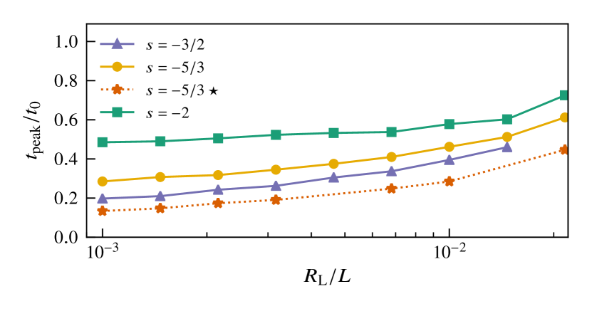
Figure 5: Dependence of $t_{\rm peak}$ on the Larmor radius $R_{\mathrm{L}}$ (expressed in units of $L$) in the test particle simulations, for different choices of the magnetic spectral index $s$. The data points shown with stars are obtained with a CR self-scattering model discussed in the text. These results show that an adequate choice of the parameter $\tau$ needs to correctly account for the energy of the modelled CR population and the form of the (subgrid) magnetic spectrum. (Data shown in Table 2.)

Table 2: Larmor radius and $t_{\text{peak}}$ for different choices of magnetic spectral index, $s$. The star indicates the run with CR self-scattering model (see text).

	$t_{\rm peak}/t_{0}$
$10^{3}R_{\text{L}}/L$	$s=-3/2$	$s=-5/3$	$s=-5/3\;\star$	$s=-2$
1.00	0.20	0.28	0.13	0.48
1.47	0.21	0.31	0.15	0.49
2.15	0.24	0.32	0.17	0.51
3.16	0.26	0.34	0.19	0.52
4.64	0.30	0.38		0.53
6.81	0.34	0.41	0.25	0.54
10.0	0.40	0.46	0.28	0.58
14.7	0.46	0.51		0.60
21.5	0.55	0.61	0.45	0.72
31.6		0.78	0.67	0.76

In the above, we have selected $R_{\mathrm{L}}$ for test particles that allows for reasonable comparison with fluid simulations. However, the dynamically important CRs in the ISM have much smaller $R_{\mathrm{L}}$. Since it appears that the time of the peak, $t_{\text{peak}}$, and $\tau$ are connected, an investigation of how $t_{\text{peak}}$ varies with particle energy (or $R_{\mathrm{L}}$) may suggest a suitable range of $\tau$ to use in more realistic fluid simulations. In this section, we perform test-particle simulations, but now utilizing the continuum model for the magnetic field described by Snodin et al. (2016), where the magnetic field is constructed in the form of Fourier series with random phases. This implementation allows one to probe much lower particle energies than the discrete mesh model used above, where the mesh spacing controls the smallest value of $R_{\mathrm{L}}$ accessible. However, it still remains impractical to faithfully explore energies much below $R_{\mathrm{L}}\lesssim 10^{-4}L$, and so one can at best extrapolate to infer the behaviour at the smallest relevant scales. This model magnetic field has fluctuations at a wide range of geometrically-spaced wave numbers to ensure sufficient resonant scattering of the particles at small scales. We take $k_{\text{max}}^{\text{particle}}/k_{\text{min}}=1024$, and $N=1024$ distinct wave vectors.

In Fig. 5 (data shown in Table 2, we show the dependence of $t_{\text{peak}}$ on $R_{\mathrm{L}}$ and on the spectral index, $s$, using a set of test particle simulations. The scaling with $R_{\mathrm{L}}$ is approximately linear in all cases. At sufficiently large $R_{\mathrm{L}}$ ($R_{\mathrm{L}}\gtrsim 0.03L$ for the values of $s$ considered here), the peaks vanish (i.e. the peak and asymptotic values coincide), so $t_{\text{peak}}$ cannot be determined. Apparently, there is a non-zero intercept at low $R_{\mathrm{L}}$, which appears to depend linearly on $s$.

At such small scales, it is expected that particles will be scattered by self-generated waves (e.g., Kulsrud & Pearce, 1969; Wentzel, 1974), which may have some effect on $t_{\text{peak}}$. In an attempt to account for this we adopt the simple scattering model used by Seta et al. (2018), which introduces an isotropic random change to the particle pitch angle with respect to the local magnetic field once per Larmor time $t_{\rm L}$. In this model, the average change in the angle is proportional to $(R_{L}/L)^{1/4}$. Applying this to the $s=-5/3$ case, we find a reduction in the intercept, but not a significant difference in the slope, as shown in Fig. 5.

4 Discussion and Conclusions

Inspection of Fig. 1 shows that the Fickian prescription for the diffusion of cosmic rays is unable to capture the transition from a ballistic to a diffusive regime, which is manifest at earlier times in test particle simulations. Nevertheless, the effective diffusivity asymptotically converges to that of the test particles using $\kappa_{\parallel}$ and $\kappa_{\perp}$ as calibrated for the Telegraph prescription.

The detailed agreement between the test-particle results and solutions of the telegraph equation in Fig. 4 is remarkable, given that the diffusion coefficients adopted are global constants that have no direct dependence on the local magnetic field properties. This suggests strongly that the telegraph equation is a viable model for simulations of cosmic ray propagation using a fluid description, with a subgrid model for their diffusion. The higher is the spatial resolution of such simulations and the larger is the particle energy, the more important can be initial deviations of the particle propagation from a diffusive behaviour at the numerically resolved scales, and the properly calibrated telegraph equation proves to be able to capture such behaviours.

Our results lead to an estimate of the time scale $\tau$, a parameter in the telegraph equation. Taking the outer scale of the turbulence $L\approx 100\,{\rm pc}$ and assuming that the dynamically important CRs (mainly protons) have energy of order $1\,{\rm GeV}$ (i.e., $R_{L}\simeq 10^{12}\,{\rm cm}$), the presence of a nonzero intercept in Fig. 5 indicates that $\tau\simeq 20\,{\rm yr}$ – under the assumption of $\tau\approx 0.5t_{\text{peak}}$ and taking ${t_{\text{peak}}\approx 0.12\times(100\,{\rm pc})/c}$, extrapolated from the self-scattering ${s=-5/3}$ case. The maximum propagation speed for disturbances in the CR fluid is related to $\tau$ and follows as ${v_{\text{max}}=(\kappa_{\parallel}/\tau)^{1/2}\simeq 10^{9}\,{\rm cm}\,{\rm s}^{-1}}$.

It is worth noticing that the asymptotic value of the global diffusivity, $\kappa_{\text{eff}}$, is about an order of magnitude smaller than the local diffusivity, $\kappa_{\parallel}$, which is applied at the mesh scale in the fluid simulation. This must be taken into account when choosing simulation parameters: to achieve a global effective diffusivity of order $10^{28}\,{\rm cm}^{2}\,{\rm s}^{-1}$ — consistent with best fits to CR observational data (Strong et al., 2007) — our results suggest that a local diffusivity of at least $\kappa_{\parallel}\sim 10^{29}\,{\rm cm}^{2}\,{\rm s}^{-1}$ needs to be adopted.

We have assumed CRs are scattered primarily by extrinsic turbulence, rather than self-generated waves that would lead to self-confinement (see, e.g., Zweibel, 2017, for a discussion of these two regimes). (For self-confined CRs, one might employ modified fluid equations, such as those of Thomas & Pfrommer 2019.) We have also neglected dynamical effects of CRs on the gas density and velocity and, thereby, on the magnetic field. It is, however, unlikely that such effects can change the nature of the CR diffusion process.

References

- Bakunin (2008) Bakunin O. G., 2008, Turbulence and Diffusion: Scaling Versus Equations. Springer-Verlag Berlin Heidelberg, doi:10.1007/978-3-540-68222-6
- Brandenburg & Dobler (2010) Brandenburg A., Dobler W., 2010, Pencil: Finite-difference Code for Compressible Hydrodynamic Flows, Astrophysics Source Code Library (ascl:1010.060)
- Farber et al. (2018) Farber R., Ruszkowski M., Yang H. Y. K., Zweibel E. G., 2018, ApJ, 856, 112
- Girichidis et al. (2016) Girichidis P., et al., 2016, ApJ, 816, L19
- Gombosi et al. (1993) Gombosi T. I., Jokipii J. R., Kota J., Lorencz K., Williams L. L., 1993, ApJ, 403, 377
- Grenier et al. (2015) Grenier I. A., Black J. H., Strong A. W., 2015, ARA&A, 53, 199
- Hanasz et al. (2009) Hanasz M., Wóltański D., Kowalik K., 2009, ApJ, 706, L155
- Holguin et al. (2018) Holguin F., Ruszkowski M., Lazarian A., Farber R., Yang H. Y. K., 2018, preprint, (arXiv:1807.05494)
- Kulsrud (2005) Kulsrud R. M., 2005, Plasma Physics for Astrophysics. Princeton University Press, Princeton
- Kulsrud & Pearce (1969) Kulsrud R., Pearce W. P., 1969, ApJ, 156, 445
- Litvinenko & Noble (2016) Litvinenko Y. E., Noble P. L., 2016, Physics of Plasmas, 23, 062901
- Litvinenko & Schlickeiser (2013) Litvinenko Y. E., Schlickeiser R., 2013, A&A, 554, A59
- Malkov & Sagdeev (2015) Malkov M. A., Sagdeev R. Z., 2015, ApJ, 808, 157
- Seta et al. (2018) Seta A., Shukurov A., Wood T. S., Bushby P. J., Snodin A. P., 2018, MNRAS, 473, 4544
- Simpson et al. (2016) Simpson C. M., Pakmor R., Marinacci F., Pfrommer C., Springel V., Glover S. C. O., Clark P. C., Smith R. J., 2016, ApJ, 827, L29
- Snodin et al. (2006) Snodin A. P., Brandenburg A., Mee A. J., Shukurov A., 2006, MNRAS, 373, 643
- Snodin et al. (2016) Snodin A. P., Shukurov A., Sarson G. R., Bushby P. J., Rodrigues L. F. S., 2016, MNRAS, 457, 3975
- Strong et al. (2007) Strong A. W., Moskalenko I. V., Ptuskin V. S., 2007, Ann. Rev. Nucl. Particle Sci., 57, 285
- Tautz & Lerche (2016) Tautz R. C., Lerche I., 2016, Res. Astron. Astrophys., 16, 162
- Thomas & Pfrommer (2019) Thomas T., Pfrommer C., 2019, MNRAS, 485, 2977
- Wentzel (1974) Wentzel D. G., 1974, ARA&A, 12, 71
- Zweibel (2013) Zweibel E. G., 2013, Phys. Plasmas, 20, 055501
- Zweibel (2017) Zweibel E. G., 2017, Phys. Plasmas, 24, 055402