Parameter Synthesis Problems for one parametric clock Timed Automata

Abstract

In this paper, we study the parameter synthesis problem for a class of parametric timed automata. The problem asks to construct the set of valuations of the parameters in the parametric timed automaton, referred to as the feasible region, under which the resulting timed automaton satisfies certain properties. We show that the parameter synthesis problem of parametric timed automata with only one parametric clock (unlimited concretely constrained clock) and arbitrarily many parameters is solvable when all the expressions are linear expressions. And it is moreover the synthesis problem is solvable when the form of constraints are parameter polynomial inequality not just simple constraint and parameter domain is nonnegative real number.

1 Introduction

Real-time applications are increasing importance, so are their complexity and requirements for trustworthiness, in the era of Internet of Things (IoT), especially in the areas of industrial control and smart homes. Consider, for example, the control system of a boiler used in house. Such a system is required to switch on the gas within a certain bounded period of time when the water gets too cold. Indeed, the design and implementation of the system not only have to guarantee the correctness of system functionalities, but also need to assure that the application is in compliance with the non-functional requirements, that are timing constraints in this case.

Timed automata (TAs) [4, 5] are widely used for modeling and verification of real-time systems. However, one disadvantage of the TA-based approach is that it can only be used to verify concrete properties, i.e., properties with concrete values of all timing parameters occurring in the system. Typical examples of such parameters are upper and lower bounds of computation time, message delay and time-out. This makes the traditional TA-based approach not ideal for the design of real-time applications because in the design phase concrete values are often not available. This problem is usually dealt with extensive trial-and-error and prototyping activities to find out what concrete values of the parameters are suitable. This approach of design is costly, laborious, and error-prone, for at least two reasons: (1) many trials with different parameter configurations suffer from unaffordable costs, without enough assurance of a safety standard because a sufficient coverage of configurations is difficult to achieve; (2) little or no feedback information is provided to the developers to help improve the design when a system malfunction is detected.

1.1 Decidable parametric timed automata

To mitigate the limitations of the TA-based approach, parametric timed automata (PTAs) are proposed [7, 11, 12, 26], which allow more general constraints on invariants of notes (or states) and guards of edges (or transitions) of an automaton. Informally, a clock $x$ of a PTA $\mathcal{A}$ is called a parametrically constrained clock if $x$ and some parameters both occur in a constraint of $\mathcal{A}$. Obviously, given any valuation of the parameters in a PTA, we obtain a concrete TA. One of the most important questions of PTAs is the parameter synthesis problem, that is, for a given property to compute the entire set of valuations of the parameters for a PTA such that when the parameters are instantiated by these valuations, the resulting TAs all satisfy the property. The synthesis problem for general PTAs is known to be undecidable. There are, however, several proposals to restrict the general PTAs from different perspectives to gain decidability. Two kinds of restrictions that are being widely investigated are (1) on the number of clocks/parameters in the PTA; and (2) on the way in which parameters are bounded, such as the L/U PTAs [26].

There are many works about parametric timed automata. An algorithm based on backward to solve nontrivial class of parametric verification problems is presented in [7]. The authors have proved that a large class of parametric verification problems are undecidable; they have also showed that the remaining (intermediate) class of parametric verification problems for which then have neither decision procedures nor undecidability results are closely related to various hard and open problems of logic and automata theory. A semi-algorithm approach based on (1) expressive symbolic representation structures is called parametric DBP’s, and (2) accurate extrapolation techniques allow to speed up the reachability analysis and help its termination is proposed in [11]. An algorithm and the tools for reachability analysis of hybrid systems is presented in [3]. They combine the notion of predicate abstraction with resent techniques for approximating the set of reachable states of linear systems using polyhedron. The main diffcult of this method is how to find the enough predicates. In [27], the authors give a method without an explicit enumeration to synthesize all the values of parameters and give symbolic algorithms for reachability and unavoidability properties. An adaptation of counterexample guided abstraction refinement (CEGAR) with which one can obtain an under approximation of the set of good parameters using linear programming is proposed in [22]. An inverse method which synthesizes the constraint of parameters for an existing trace such that it can guarantee its executes of parametric timed automata under this constraint with same previous trace is provided in [9]. In [27], the authors provide a subclass of parametric timed automata which they can actually and efficiently analyze. The author of [8] makes a survey of decision and computation problems progress based on the recent 25 years’ researches on these problems.

The constraints in above works are simple constraint which means that in the form of constraint as $x\prec c$ ($x-y\prec c$), $x\prec p$ ($x-y\prec p$) or logical combination of above forms where $x,y$ are clocks, $c$ is a constant and $p$ is parameter. In this paper, we will extended the form to $x\prec f(p_{1},\cdots,p_{m})$ ($x-y\prec f(p_{1},\cdots,p_{m})$) where $p_{1},\cdots,p_{m}$ are parameters and $f$ is a polynomial in $\mathbb{Z}[p_{1},\cdots,p_{m}]$.

There are many works related to solving polynomial constraints problems e.g. [31, 18].

As one would expect, Tarski’s procedure consequently has been much im- proved. Most notably, Collins [18] gave the first relatively effective method of quantifier elimination by cylindrical algebraic decomposition (CAD). The CAD procedure itself has gone through many revisions [19, 25, 29, 30, 15, 20, 23]. The CAD algorithm works by decomposing $\mathbb{R}^{k}$ into connected components such that, in each cell, all of the polynomials from the problem are sign-invariant. To be able to perform such a particular decomposition, CAD first performs a projection of the polynomials from the initial problem. This projection includes many new polynomials, derived from the initial ones, and these polynomials carry enough information to ensure that the decomposition is indeed possible. Unfortunately, the size of these projections sets grows exponentially in the number of variables, causing the projection phase to be a key hurdle to CAD scalability.

1.1.1 Contribution

In this paper, we study the parameter synthesis problem of a class of parametric time automata. We show that the parameter synthesis problem of parametric timed automata with only one parametric clock (unlimited concretely constrained clock) and arbitrarily many parameters is solvable when all the expressions are linear expressions. And it is moreover the synthesis problem is solvable when the form of constraints are parameter polynomial inequality and parameter domain is nonnegative real number.

Table 1: Our PTA results

$\mathbb{T}$	$\mathbb{P}$	Constraints	P-clocks	NP-clocks	Params	emptiness	synthesis
$\mathbb{N}$	$\mathbb{R}$	Polynomial constraints	1	0	any		solvable
$\mathbb{N}$	$\mathbb{Z}$	Simple constraints	1	any	any		solvable

• “$\mathbb{T}$” to denote the domain of clock.

• “$\mathbb{P}$” to denote the domain of parameter.

• “Constraints” is form of constraint in PTA include constraints occurring in property.

• “P-clocks” is the number of parametric clock.

• “NP-clocks” is the number of concretely constrained clock.

• “Params” is the number of parameters occurring in PTA.

• “emptiness” denote the whether decidable of emptiness problem.

• “synthesis” denote the whether decidable of synthesis problem.

1.1.2 Related work

Besides the above mentioned works, there are several other results that related to ours. The idea of limiting the number of parameters used such that upper and lower bounds cannot share a same parameter is also presented in [6] where the authors studied the logic LTL augmented with parameters. And our topic parametric timed automata is different from theirs. An extension of the model checker UPPAAL presented in [26] is capable of synthesizing linear parameter constraints for the correctness of parametric timed automata and it also identifies a subclass of parametric timed automata  (L/U automata) for which the emptiness problem is decidable. Decidability results for L/U automata have been further investigated in [14] where the constrained versions of emptiness and universality of the set of parameter valuations for which there is a corresponding infinite accepting run of the automaton is studied and decidability if parameters of different types (lower and upper bound parameters) are not compared in the linear constraint is obtained. They show how to compute the explicit representation of the set of parameters when all the parameters are of the same type (L-automata and U-automata). Compared with [14] which considers liveness problems of the system, our results are related to synthesis parameter which satisfies a given property. In [16], the authors show that the model-checking problem is decidable and the parameter synthesis problem is solvable, in discrete time, over a PTA with one parametric clock, if equality is not allowed in the formula. Compared with it, we do not have equality restriction. In [10], the authors proved that the language-preservation problem is decidable for deterministic for the parametric timed automata with all lower bound parameters or all upper bound parameters and one parameter. However, the limitations we consider for obtaining decidability is orthogonal to those presented in [10]. In [17], the authors prove that the emptiness problem of parametric timed automata with two parameter clocks and one parameter is decidable.

1.1.3 Organization

After the introduction, the definition of parametric timed automata is presented in Section 2. In Section 3 some theoretical results about parameter synthesis problem are given. Based on result of CAD we prove that with only one parametric clock and arbitrarily many parameters is solvable. And it is moreover the form of constraints are parameter polynomial inequality. In Section 4, We show that the parameter synthesis problem of parametric timed automata with only one parametric clock (unlimited concretely constrained clock) and arbitrarily many parameters is solvable when all the expressions are linear expressions.

2 Parametric Timed Automata

We introduce the basis of PTAs and set up terminology for our discussion. We first define some preliminary notations before we introduce PTAs. We will use a model of labeled transition systems (LTS) to define semantic behavior of PTAs.

2.1 Preliminaries

We use $\mathbb{Z}$, $\mathbb{N}$, $\mathbb{R}$ and $\mathbb{R}^{+}$ to denote the sets of integers, natural numbers, real numbers and non-negative real numbers, respectively. Although each PTA involves only a finite number of clocks and a finite number parameters, we need an infinite set of clock variables (also simply called clocks), denoted by $\mathcal{X}$ and an infinite set of parameters, denoted by $\mathcal{P}$, both are enumerable. We use $X$ and $P$ to denote (finite) sets of clocks and parameters and $x$ and $p$, with subscripts if necessary, to denote clocks and parameters, respectively. We use $\mathbb{T}$ to denote the domain of clocks. We are mostly interested in the case that $\mathbb{T}=\mathbb{N}$ or $\mathbb{T}=\mathbb{R}^{+}$ of nonnegative reals. Unless explicitly specified, our results are applicable in either case. We use $\mathbb{P}$ to denote the domain of clocks. We are mostly interested in the case that $\mathbb{P}=\mathbb{Z}$ or $\mathbb{P}=\mathbb{R}$.

We mainly consider dense time, and thus we define a clock valuation $\omega$ as a function of the type $\mathcal{X}\mapsto\mathbb{T}$. For a finite set $X=\{x_{1},\ldots,x_{n}\}$ of clocks, an evaluation $\omega$ restricted on $X$ can be represented by a $n$-dimensional point $\omega(X)=(\omega(x_{1}),\omega(x_{2}),\ldots,\omega(x_{n}))$, and it is called an parameter valuation of $X$ and simply denoted as $\omega$ when there is no confusion. Given a constant $d\in\mathbb{T}$, we use $\omega+d$ to denote the evaluation that assigns any clock $x$ with the value $\omega(x)+d$, and $(\omega+d)(X)=(\omega(x_{1})+d,\omega(x_{2})+d,\ldots,\omega(x_{n})+d)$. When $n=1$, we directly use $\omega$ as the value of clock $x_{1}$. Similarly, a parameter valuation $\gamma$ is an assignment of values to the parameters, that is $v:\mathcal{P}\mapsto\mathbb{P}$. For a finite set $P=\{p_{1},\ldots,p_{m}\}$ of $m$ parameters, a parameter valuation $\gamma$ restricted on $P$ corresponds to a $m$-dimensional point $(\gamma(p_{1}),\gamma(p_{2}),\ldots,\gamma(p_{m}))\in\mathbb{P}^{m}$, and we use this vector to denote the valuation $\gamma$ of $P$ when there is no confusion. When $m=1$, we directly use $\gamma$ as the value of $p_{1}$.

Definition 1 (Expression)

A linear expression $e$ is either an expression of the form $c_{0}+c_{1}p_{1}+\cdots+c_{n}p_{n}$ where $c_{0},\cdots,c_{n}\in\mathbb{Z}$, or $\infty$. We use ${\tt cf}(e,p)$ to denote the coefficient of $p$ in linear expression $e$. A polynomial expression is an expression of the form $\sum_{i=0}^{h}c_{i}p_{1}^{k_{i,1}}c\cdots p_{m}^{k_{i,m}}$ where $c_{0},\cdots,c_{h}\in\mathbb{Z},k_{i,j}\in\mathbb{N}$.

We also write polynomial $f$ as form

$$f(Y,x)=c_{l}^{\prime}p_{m}^{d_{l}}+c_{l-1}^{\prime}p_{m}^{d_{l-1}}+\cdots+c_{1}^{\prime}p_{m}^{\prime d_{1}}+c_{0}^{\prime}$$

where $Y=[y_{1},\cdots,y_{k}],\ 0<d_{1}<\cdots<d_{l}$, and the coefficients $c_{i}^{\prime}$ are in $\mathbb{Z}[y_{1},\cdots,y_{k}]$ with $c_{l}^{\prime}\neq 0$.

We use $\mathcal{LE}$ and $\mathcal{PE}$ to denote the set of linear expressions and polynomial expression, respectively. We use $\mathcal{E}$ to denote set $\mathcal{LE}\cup\mathcal{PE}$. For an $e\in\mathcal{LE}$, we use $\textit{con}(e)$ the constant $c_{0}$, and ${\tt cf}(e,p)$ the coefficient of $p$ in $e$, i.e. $c_{i}$ if $p$ is $p_{i}$ for $i=1,\ldots,m$, and $0$, otherwise. For the convenience of discussion, we also say the infinity $\infty$ is a expression. We call expression $e$ a parametric expression if it contains some parameter, a concrete expression, otherwise (i.e., $e$ is parameter free).

A PTA only allows parametric constraints of the form $x-y\sim e$, where $x$ and $y$ are clocks, $e$ is an expression, and the ordering relation $\sim\in\{>,\geq,<,\leq,=\}$. A constraint $g$ is called a parameter-free (or concrete) constraint if the expression in it is concrete. For an expression $e$, a parameter valuation $\gamma$, a clock valuation $\omega$ and a constraint $g$, let

• $e[\gamma]$ be the (concretized) expression obtained from $e$ by substituting the value $\gamma(p_{i})$ for $p_{i}$ in $e$, i.e. when $e$ is a linear expression $e=c_{0}+c_{1}p_{1}+\cdots,c_{m}p_{m}$, then $e[\gamma]=c_{0}+c_{1}\times\gamma(p_{1})+\ldots+c_{m}\times\gamma(p_{m})$,

• $g[\gamma]$ be the predicate obtained from constraint $g$ by substituting the value $\gamma(p_{i})$ for $p_{i}$ in $g$, and

• $\omega\models g$ holds if $g[\omega]$ holds.

A pair $(\gamma,\omega)$ of parameter valuation and clock valuation gives an evaluation to any parametric constraint $g$. We use $g[\gamma,\omega]$ to denote the truth value of $g$ obtained by substituting each parameter $p$ and each clock $x$ by their values $\gamma(p)$ and $\omega(x)$, respectively. We say the pair of valuations $(\gamma,\omega)$ satisfies constraint $g$, denoted by $(\gamma,\omega)\models g$, if $g[\gamma,\omega]$ is evaluated to true. For a given parameter valuation $\gamma$, we define $[\![g[\gamma]]\!]=\{\omega\mid(\gamma,\omega)\models g\}$ to be the set of clock valuations which together with $\gamma$ satisfy $g$.

A clock $x$ is reset by an update which is an expression of the form $x:=b$, where $b\in\mathbb{N}$. Any reset $x:=b$ will change a clock valuation $\omega$ to a clock valuation $\omega^{\prime}$ such that $\omega^{\prime}(x)=b$ and $\omega^{\prime}(y)=\omega(y)$ for any other clock $y$. Given a clock valuation $\omega$ and a set $u$ of updates, called an update set, which contains at most one reset for one clock, we use $\omega[u]$ to denote the clock valuation after applying all the clock resets in $u$ to $\omega$. We use $c[u]$ to denote the constraint which is used to assert the relation of the parameters with the clocks values after the clock resets of $u$. Formally, $c[u](\omega)\ \widehat{=}\ c(\omega[u])$ for every clock valuation $\omega$.

It is easy to see that the general constraints $x-y\sim e$ can be expressed in terms of atomic constraints of the form $b_{1}x-b_{2}y\prec e$, where $\prec\in\{<,\leq\}$ and $b_{1},b_{2}\in\{0,1\},e\in\mathcal{E}$. To be explicit, an atomic constraint is in one of the following three forms $x-y\prec e$, $x\prec e$, or $-x\prec e$. We can write $-x_{i}\prec e$ as $x_{i}\succ-e$. and $x-y\prec e$ as $y-x\succ-e$, where $\succ\in\{>,\geq\}$. However, in this paper we mainly consider simple constraints that are finite conjunctions of atomic constraints.

2.2 Parametric timed automata

We assume the knowledge of timed automata (TAs), e.g., [2, 13]. A clock constraint of a TA either a invariant property when the TA is in a state (or location) or a guard condition to enable the changes of states (or a state transition). Such a constraint is in general a Boolean expression of parametric free atomic constraints. However, we can assume that the guards and invariants of TA are simple concrete constraints, i.e. conjunctions of concrete atomic constraints. This is because we can always transform a TA with disjunctive guards and invariants to an equivalent TA with guards and invariants which are simple constraints only.

In what follows, we define PTAs which extend TAs to allow the use of parametric simple constraints as guards and invariants (see [7]).

Definition 2 (PTA)

Given a finite set of clocks $X$ and a finite set of parameters $P$, a PTA is a 5-tuple $\mathcal{A}=(\Sigma,Q,q_{0},I,\rightarrow)$, where

• $\Sigma$ is a finite set of actions.

• $Q$ is a finite set of locations and $q_{0}\in Q$ is called the initial location,

• $I$ is the invariant, assigning to every $q\in Q$ a simple constraint $I_{q}$ over the clocks $X$ and parameters $P$, and

• $\rightarrow$ is a discrete transition relation whose elements are of the form $(q,g,a,u,q^{\prime})$, where $q,q^{\prime}\in Q$, $u$ is an update set, $a\in\Sigma$ and $g$ is a simple constraint.

Given a PTA $\mathcal{A}$, a tuple $(q,g,a,u,q^{\prime})\in\rightarrow$ is also denoted by $q\xrightarrow{g\&a[u]}q^{\prime}$, and it is called a transition step (by the guarded action $g\&a$). In this step, $a$ is the action that triggers the transition. The constraint $g$ in the transition step is called the guard of the transition step, and only when $g$ holds in a location can the transition take place. By this transition step, the system modeled by the automaton changes from location $q$ to location $q^{\prime}$, and the clocks are reset by the updates in $u$. However, the meaning of the guards and clock resets and acceptable runs of a PTA will be defined by a labeled transition system (LTS) later on. At this moment, we define a syntactic run of a PTA $\mathcal{A}$ as a sequence of consecutive transitions step starting from the initial location

$$\tau=(q_{0},I_{q_{0}})\xrightarrow{g_{1}\&a_{1}[u_{1}]}(q_{1},I_{q_{1}})\cdots\xrightarrow{g_{\ell}\&a_{\ell}[u_{\ell}]}(q_{\ell},I_{q_{\ell}}).$$

We call a syntactic run $\tau$ is a simple syntactic run if $\tau$ has no location variants and clock resets.

Given a PTA $\mathcal{A}$, a clock $x$ is said to be a parametrically constrained clock in $\mathcal{A}$ if there is a parametric constraint containing $x$. Otherwise, $x$ is a concretely constrained clock. We can follow the procedures in [7] and [17] to eliminate from $\mathcal{A}$ all the concretely constrained clocks. Thus, the rest of this paper only considers the PTAs in which all clocks are parametrically constrained. We use $\textit{expr}(\mathcal{A})$ and $\textit{para}(\mathcal{A})$ to denote the set of all expressions and parameters in a PTA $\mathcal{A}$, respectively.

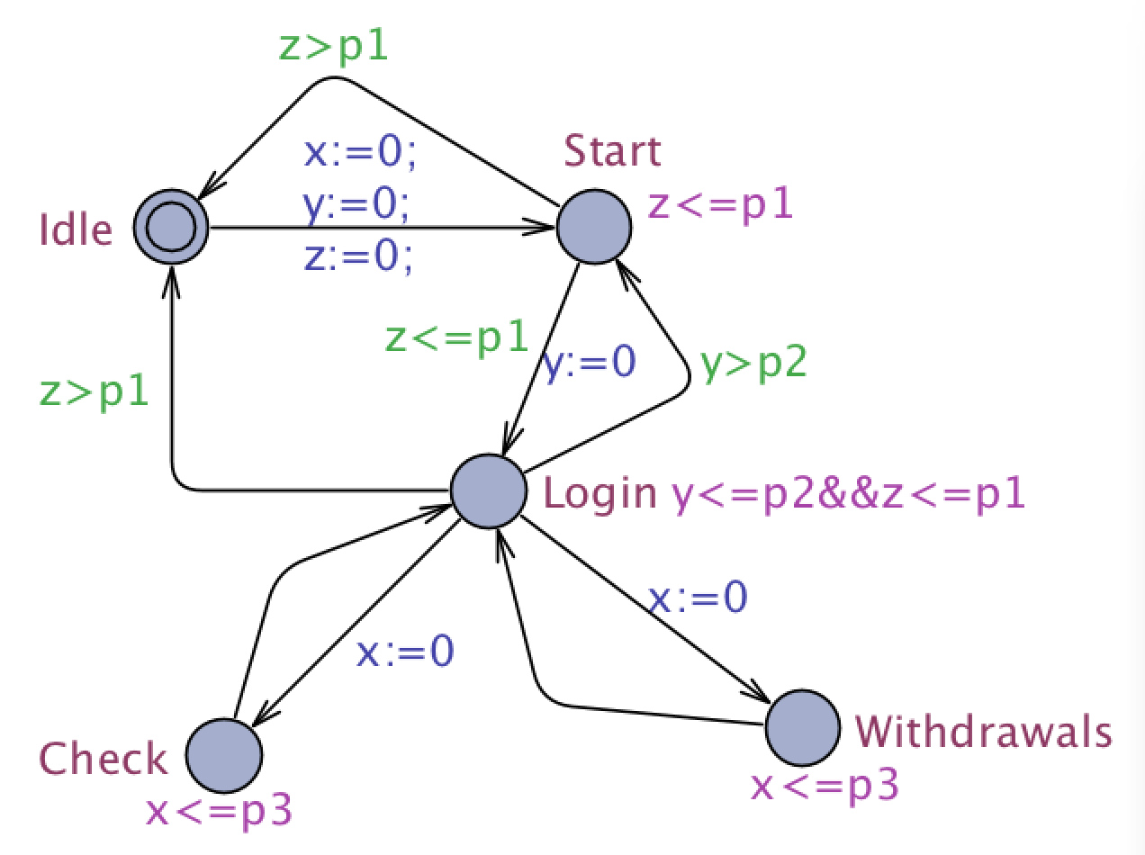
Figure 1: An ATM modeled using a PTA.

Example 1

The PTA in Fig. 1 models an ATM. It has 5 locations, 3 clocks $\{x,y,z\}$ and 3 parameters $\{p_{1},p_{2},p_{3}\}$. This PTA is deterministic and all the clocks are parametric. To understand the behavior of state transitions, for examples, the machine can initially idle for an arbitrarily long time. Then, the user can start the system by, say, pressing a button and the PTA enters location “Start” and resets the three clocks. The machine can remain in “Start” location as long as the invariant $z\leq p_{1}$ holds, and during this time the user can drive the system (by pressing a corresponding button) to login their account and the automaton enters location “Login” and resets clock $y$. A time-out action occurs and it goes back to “Idle” if the machine stays at “Start” for too long and the invariant $z\leq p_{1}$ becomes false. Similarly, the machine can remain in location “Login” as long as the invariant $y\leq p_{2}\wedge z\leq p_{1}$ holds and during this time the user can decide either to “Check” (her balance) or to “Withdraw” (money), say by pressing corresponding buttons. However, if the user does not take any of these actions $p_{2}$ time units after the machine enter location “Login”, the machine will back to “Start” location.

2.3 Semantics of PTA via labeled transition systems

We use a standard model of labeled transition systems (LTS) for describing and analyzing the behavioral properties of PTA.

Definition 3 (LTS)

A labeled transition system (LTS) over a set of (action) symbols $\Delta$ is a triple $\mathcal{L}=(S,S_{0},\rightarrow)$, where

• $S$ is a set of states with a subset $S_{0}\subseteq S$ of states called the initial states.

• $\rightarrow\subseteq S\times\Delta\times S$ is a relation, called the transition relation.

We write $s\xrightarrow{a}s^{\prime}$ for a triple $(s,a,s^{\prime})\in\rightarrow$ and it is called a transition step by action $a$.

A run of $\mathcal{L}$ is a finite alternating sequence of states in $S$ and actions $\Delta$, $\xi=s_{0}a_{1}s_{1}\ldots a_{\ell}s_{\ell}$, such that $s_{0}\in S_{0}$ and $s_{i-1}\xrightarrow{a_{i}}s_{i}\in\rightarrow$ for $i=1,\ldots,\ell$. A run $\xi$ can be written in the form of $s_{0}\xrightarrow{a_{1}}s_{1}\xrightarrow{a_{2}}\cdots\xrightarrow{a_{\ell}}s_{\ell}$. The length of a run $\xi$ is its number $\ell$ of transitions steps and it is denoted as $|\xi|$, and a state $s\in S$ is called reachable in $\mathcal{L}$ if $s$ is the last state a run of $\mathcal{L}$, e.g. $s_{\ell}$ of $\xi$.

Definition 4 (LTS semantics of PTA)

For a PTA $\mathcal{A}=(\Sigma,Q,q_{0},I,\rightarrow)$ and a parameter valuation $\gamma$, the concrete semantics of PTA under $\gamma$, denoted by $\mathcal{A}[\gamma]$, is the LTS $(S,S_{0},\rightarrow)$ over $\Sigma\cup\mathbb{R}^{+}$, where

• a state in $S$ is a location $q$ of $\mathcal{A}$ augmented with the clock valuations which together with the parameter valuation $\gamma$ satisfy the invariant $I_{q}$ of the location, that is

  $$S=\{(q,\omega)\in Q\times(X\rightarrow\mathbb{R}^{+})\mid(\gamma,\omega)\models I_{q}\}$$

  $$S_{0}=\{(q_{0},\omega)\mid(\gamma,\omega)\models I_{q_{0}}\wedge\omega=(0,\cdots,0)\}$$

• any transition step in the transition $\rightarrow$ of the LTS is either an instantaneous transition step by an action in $\Sigma$ defined by $\mathcal{A}$ or by a time advance, that are specified by the following rules, respectively

  • instantaneous transition: for any $a\in\Sigma$, $(q,\omega)\xrightarrow{a}(q^{\prime},\omega^{\prime})$ if there are simple constraint $g$ and an update set $u$ such that $q\xrightarrow{g\&a[u]}q^{\prime}$, $(\gamma,\omega)\models g$ and $\omega^{\prime}=\omega[u]$; and

  • time advance transition $(q,\omega)\xrightarrow{d}(q^{\prime},\omega^{\prime})$ if $q^{\prime}=q$ and $\omega^{\prime}=\omega+d$.

A concrete run of a PTA $\mathcal{A}$ for a given valuation $\gamma$ is a sequence of consecutive state transition steps $\xi=s_{0}\xrightarrow{t_{1}}s_{1}\xrightarrow{t_{2}}\cdots\xrightarrow{t_{\ell}}s_{\ell}$ of the LTS $\mathcal{A}[\gamma]$, which we also call a run of the LTS $\mathcal{A}[\gamma]$. A state $s=(q,\omega)$ of $\mathcal{A}[\gamma]$ is a reachable state of $\mathcal{A}[\gamma]$ if there exists some run $\xi=s_{0}\xrightarrow{t_{1}}s_{1}\xrightarrow{t_{2}}\cdots\xrightarrow{t_{\ell}}s_{\ell}$ of $\mathcal{A}[\gamma]$ such that $s=s_{\ell}$.

Without the loss of generality, we merge any two consecutive time advance transitions respectively labelled by $d_{i}$ $d_{i+1}$ into a single time advance transition labels by $d_{i}+d_{i+1}$. We can further merger a consecutive pair $s\xrightarrow{d}s^{\prime}\xrightarrow{a}s^{\prime\prime}$ of a timed advance transition by $d$ and an instantaneous transition by an action $a$ in a run into a single observable transition step $s\xrightarrow{a}s^{\prime\prime}$. If we do this repeatedly until all time advance steps are eliminated, we obtain an untimed run of the PTA (and the LTS), and the sequence of actions in an untimed run is called a trace.

We call an untimed run $\xi=s_{0}\xrightarrow{a_{1}}s_{1}\cdots\xrightarrow{a_{\ell}}s_{\ell}$ a simple run if $\omega_{i}\geq\omega_{i-1}$ for $i=1,\cdots,\ell$, where $s_{i}=(q_{i},\omega_{i})$. It is easy to see that $\xi$ is a simple untimed run if each transition by $a_{i}$ does not have any clock reset in $\xi$.

Definition 5 (LTS of trace)

For a PTA $\mathcal{A}$ and a syntactic run

$$\tau=(q_{0}{,}I_{q_{0}})\xrightarrow{g_{1}\&a_{1}[u_{1}]}(q_{1}{,}I_{q_{1}}){\cdots}\xrightarrow{g_{\ell}{\&}a_{\ell}[u_{\ell}]}(q_{\ell}{,}I_{q_{\ell}})$$

we define the PTA $\mathcal{A}_{\tau}{=}(\Sigma_{\tau}{,}Q_{\tau}{,}q_{0,\tau}{,}I_{\tau},\rightarrow_{\tau})$, where

• $\Sigma_{\tau}=\{a_{i}\mid i=1,\cdots,\ell\}$,

• $Q_{\tau}=\{q_{0},\cdots,q_{\ell}\}$ and $q_{0,\tau}=q_{0}$,

• $I_{\tau}(i)=I_{q_{i}}$ for $i\in Q$, and

• $\rightarrow_{\tau}=\{(q_{i-1},g_{i},a_{i},u_{i},q_{i})\mid i=1,\cdots,\ell\}$.

Give a parameter valuation $\gamma$, the concrete semantics of $\tau$ under $\gamma$ is defined to be the LTS $\mathcal{A}_{\tau}[\gamma]$.

For a syntactic run

$$\tau=(q_{0}{,}I_{q_{0}})\xrightarrow{g_{1}\&a_{1}[u_{1}]}(q_{1}{,}I_{q_{1}}){\cdots}\xrightarrow{g_{\ell}{\&}a_{\ell}[u_{\ell}]}(q_{\ell}{,}I_{q_{\ell}})$$

We use $R(\mathcal{A}_{\tau}[\gamma])$ to denote the set of states $(q_{k},\omega_{k})$ of $\mathcal{A}_{\tau}[\gamma]$ such that the following is an untimed run of $\mathcal{A}_{\tau}[\gamma]$

$$\xi=(q_{0},\omega_{0})\xrightarrow{a_{1}}(q_{1},\omega_{1})\cdots\xrightarrow{a_{k}}(q_{k},\omega_{k})\cdots\xrightarrow{a_{\ell}}(q_{\ell},\omega_{\ell}).$$

We also call $\xi$ is a run of syntactic run $\tau$ under $\gamma$. We use $\Gamma(\mathcal{A}_{\tau})$ to denote the entire set of parameter valuation $\gamma$ which makes $R(\mathcal{A}_{\tau}[\gamma])\neq\emptyset$.

2.4 Two decision problems for PTA

We first present the properties of PTAs which we consider in this paper.

Definition 6 (Properties)

A state property and a system property for a PTA are specified by a state predicate $\phi$ and a temporal formula $\psi$ defined by the following syntax, respectively: for $x,y\in X$, $e\in\mathcal{E}$ and $\prec\in\{<,\leq,=\}$ and $q$ is a location.

$$\begin{array}[]{lllll}\phi&::=&x\prec e\mid-x\prec e\mid x-y\prec e\mid q\mid\neg\phi\mid\phi\wedge\phi\mid\phi\vee\phi\\ \psi&::=&\forall\Box\phi\mid\exists\Diamond\phi\end{array}$$

Let $\gamma$ be a parameter valuation and $\phi$ be a state formula. We say $\mathcal{A}[\gamma]$ satisfies $\exists\Diamond\phi$, denoted by $\mathcal{A}[\gamma]\models\exists\Diamond\phi$, if there is a reachable state $s$ of $\mathcal{A}[\gamma]$ such that $\phi$ holds in state $s$. Similarly, $\mathcal{A}[\gamma]$ satisfies $\forall\Box\phi$, denoted by $\mathcal{A}[\gamma]\models\forall\Box\phi$, if $\phi$ holds in all reachable states of $\mathcal{A}[\gamma]$. We can see that if $\mathcal{A}[\gamma]{\models}\exists\Diamond\phi$, there is an syntactic run $\tau$ such that there is a state in $R(\mathcal{A}_{\tau}[\gamma])$ satisfies $\phi$. In this case, we also say that the syntactic run $\tau$ satisfies $\phi$ under the parameter valuation $\gamma$. We denote it by $\tau[\gamma]\models\phi$.

We are now ready to present the formal statement of the parameter synthesis problem and the emptiness problem of PTA.

Problem 1 (The parameter synthesis problem)

Given a PTA $\mathcal{A}$ and a system property $\psi$, compute the entire set $\Gamma(\mathcal{A},\psi)$ of parameter valuations such that $\mathcal{A}[\gamma]\models\psi$ for each $\gamma\in\Gamma(\mathcal{A},\psi)$.

Solutions to the problems are important in system plan and optimization design. Notice that when there are no parameters in $\mathcal{A}$, the problem is decidable in PSPACE [5]. This implies that if there are parameters in $\mathcal{A}$, the satisfaction problem $\mathcal{A}[\gamma]\models\psi$ is decidable in PSPACE for any given parameter valuation $\gamma$.

A special case of the synthesis problem is the emptiness problem, which is by itself very important and formulated below.

Problem 2 (Emptiness problem)

Given a PTA $\mathcal{A}$ and a system property $\psi$, is there a parameter valuation $\gamma$ so that $\mathcal{A}[\gamma]\models\psi$?

This is equivalent to the problem of checking if the set $\Gamma(\mathcal{A},\psi)$ of feasible parameter valuations is empty.

Many safety verification problems can be reduced to the emptiness problem. We say that Problem 2 is a special case of Problem 1 because solving the latter for a PTA $\mathcal{A}$ and a property $\psi$ solves Problem 2.

It is known that the emptiness problem is decidable for a PTA with only one clock [7]. However, the problem becomes undecidable for PTAs with more than two clocks [7]. Significant progress could only be made in 2002 when the subclass of L/U PTA were proposed in [26] and the emptiness problem was proved to be decidable for these automata. In the following, we will extend these results and define some classes of PTAs for which we propose solutions to the parameter synthesis problem and the emptiness problem.

3 Parametric timed automata with one parametric clock

In this section we consider parameter synthesis problem of PTA with one parametric clock and arbitrarily many parameters. The time values $\mathbb{T}=\mathbb{N}$ and parameter values $\mathbb{P}=\mathbb{R}$. We first provide some result of CAD, then prove the synthesis problem of PTA with one parametric clock is solvable.

3.1 Cylindrical Algebraic Decomposition

Delineability plays a crucial role in the theory of CAD. Following the terminology used in CAD, we say a connected subset of $\mathbb{R}^{m}$ is a region. Given a region $S$, the cylinder $Z$ over $S$ is $S\times\mathbb{R}$. A $\theta$-section of $Z$ is a set of points $\left<{\vec{\alpha}},\theta({\vec{\alpha}})\right>$, where ${\vec{\alpha}}$ is in $S$ and $\theta$ is continuous function from $S$ to $\mathbb{R}$. A $(\theta_{1},\theta_{2})$-sector of $Z$ is the set of points $\left<{\vec{\alpha}},\beta\right>$, where ${\vec{\alpha}}$ is in $S$ and $\theta_{1}({\vec{\alpha}})<\beta<\theta_{2}({\vec{\alpha}})$ for continuous functions $\theta_{1}<\theta_{2}$ from $S$ to $\mathbb{R}$. Sections and sectors are also regions. Given a subset of $S$ of $\mathbb{R}^{m}$, a decomposition of $S$ is a finite collection of disjoint regions $S_{1},\cdots,S_{k}$ such than $S_{1}\cup\cdots\cup S_{k}=S$. Given a region $S$, and a set of continuous functions $\theta_{1}<\cdots<\theta_{k}$ from $S$ to $\mathbb{R}$, we can decompose the cylinder $S\times\mathbb{R}$ into the following regions:

• the $\theta_{i}$-sections, for $1\leq i\leq k$, and

• $(\theta_{i},\theta_{i+1})$-sections, for $0\leq i\leq k$,

where, with sight abuse of notation, we define $\theta_{0}$ as the constant function that return $-\infty$ and $\theta_{k+1}$ the constant function that return $\infty$. A set of polynomials $\{f_{1},\cdots,f_{s}\}\subset\mathbb{Z}[P,x],$ $P=[p_{1},\cdots,p_{m}]$, is said to be delineable in a region $S\subset\mathbb{R}^{m-1}$ if the following conditions hold:

1. For every $1\leq i\leq s$, the total number of complex roots of $f_{i}({\vec{\alpha}},x)$ remains invariant for any ${\vec{\alpha}}\in S$.

2. For every $i\leq i\leq s$, the number of distinct complex roots of $f_{i}({\vec{\alpha}},x)$ remains invariant for any ${\vec{\alpha}}$ in $S$.

3. For every $1\leq i<j\leq s$, the number of common complex roots of $f_{i}({\vec{\alpha}},x)$ and $f_{j}({\vec{\alpha}},x)$ remains invariant for any ${\vec{\alpha}}$ in $S$.

A sign assignment for a set of polynomials $F$ is a mapping $\delta$, from polynomials in $F$ to $\{-1,0,1\}$. Given a set of polynomials $F\subset\mathbb{Z}[P,p]$, we say a sign assignmemnt $\delta$ is realizable with respect to some ${\vec{\alpha}}$ in $\mathbb{R}^{m}$ , if there exists a $\beta\in\mathbb{R}$ such that every $f\in F$ takes the sign corresponding to its sign assignment, i.e., sgn$(f({\vec{\alpha}},\beta))=\delta(f)$. The function sgn maps a real number to its sign $\{-1,0,1\}$. We use ${\tt signs}(F,{\vec{\alpha}})$ to denote the set of realizable sign assignments of $F$ with respect to ${\vec{\alpha}}$.

Theorem 3.1 (Lemma 1 of [28])

If a set of polynomials $F\subset\mathbb{Z}[P,x]$ is delineable over a region $S$, then ${\tt signs}(F,{\vec{\alpha}})$ is invariant over $S$.

Theorem 3.2 (Main algorithm of [18])

$F$ is a set of polynomials in $\mathbb{Z}[P,x]$, there is a algorithm which computes decomposition $\mathbb{R}^{m}$ $S_{1},\cdots,S_{k}$ such that $F$ is delineable over $S_{i}$ for $i=1,\cdots,k$.

Lemma 1

For a polynomials formula $\phi$ where each polynomial of $\phi$ in $\mathbb{Z}[P,x]$, there is a decomposition $S_{1},\cdots,S_{k}$ of $\mathbb{R}^{m}$ such that $\phi$ is true or false for each point of $S_{i}$ for $i=1,\cdots,k$. Moreover, CAD  provides a sample point ${\vec{\alpha}}_{i}$ where ${\vec{\alpha}}_{i}\in S_{i}$ for $i=1,\cdots,k$.

3.2 Parametric timed automata with one parametric clock

The establishment and proof of this theorem involve a sequence of techniques to reduce the problem to computing the set of reachable states of an LTS. The major steps of reduction include

1. Reduce the problem of satisfaction of a system property $\psi$, say in the form of $\exists\Diamond\phi$, by a run $\tau$ to a reachability problem. This is done by encoding the state property in $\psi$ as a conjunction of the invariant of a state.

2. Then we move the state invariants in a run out of the states and conjoin them to the guards of the corresponding transitions.

3. Construct feasible runs for a given syntactic run in order to reach a given location. This requires to define the notions of lower and upper bounds of guards of transitions, through which an lower bound of feasible parameter valuation is defined.

3.3 Reduce satisfaction of system to reachability problem

We note that $\psi$ is either of the form $\exists\Diamond\phi$ or the dual form $\forall\Box\phi$, where $\phi$ is a state property. Therefore, we only need to consider the problem of computing the set $\Gamma(\mathcal{A},\psi)$ for the case when $\psi$ is a formula of the form $\exists\Diamond\phi$, i.e., there is a syntactic run $\tau$ such that $\tau[\gamma]\models\phi$ for every $\gamma\in\Gamma(\mathcal{A},\psi)$. Our idea is to reduce the problem of deciding $\mathcal{A}\models\psi$ to a reachability problem of an LTS by encoding the state property $\phi$ in $\exists\Diamond\phi$ into the guards of the transitions of $\mathcal{A}$.

Definition 7 (Encoding state property)

Let $\phi$ be a state formula and $q$ be a location. We definite $\alpha(\phi,q)$ as follows, where $\equiv$ is used to denote syntactic equality between formulas:

• $\alpha(\phi,q)\equiv\phi$ if $\phi\equiv x-y\prec e$, $\phi\equiv x\prec e$ or $\phi\equiv-x\prec e$, where $x$ and $y$ are clocks and $e$ is an expression.

• when $\phi$ is a location $q^{\prime}$, $\alpha(\phi,q^{\prime})\equiv true$ if $q^{\prime}$ is $q$ and $false$ otherwise.

• $\alpha$ preserves all Boolean connectives, that is $\alpha(\neg\phi_{1},q)\equiv\neg\alpha(\phi_{1},q)$, $\alpha(\phi_{1}\wedge\phi_{2},q)\equiv\alpha(\phi_{1},q)\wedge\alpha(\phi_{2},q)$, and $\alpha(\phi_{1}\vee\phi_{2},q)\equiv\alpha(\phi_{1},q)\vee\alpha(\phi_{2},q)$.

We can easily prove the following lemma.

Lemma 2

Given a PTA $\mathcal{A}$, $\psi\equiv\exists\Diamond\phi$, and a syntactic run of $\mathcal{A}$

$$\tau=(q_{0},I_{q_{0}})\xrightarrow{g_{1}\&a_{1}[u_{1}]}(q_{1},I_{q_{1}}){\cdots}\xrightarrow{g_{\ell}\&a_{\ell}[u_{\ell}]}(q_{\ell},I_{q_{\ell}})$$

we overload the function notation $\alpha$ and define the encoded run $\alpha(\tau)$ to be

$$(q_{0},I_{q_{0}})\xrightarrow{g_{1}\&a_{1}[u_{1}]}(q_{1}{,}I_{q_{1}}){\cdots}\xrightarrow{g_{\ell}\&a_{\ell}[u_{\ell}]}(q_{\ell}{,}I_{q_{\ell}}{\wedge}\alpha(\phi{,}q_{\ell}))$$

Then $\tau$ satisfies $\psi$ under parameter valuation $\gamma$ if and only if $R(\mathcal{A}_{\alpha(\tau)}[\gamma])\neq\emptyset$.

Notice the term guard is slightly abused in the lemma as $\alpha(\phi,q_{\ell})$ may have disjunctions, and thus it may not be a simple constraint.

3.4 Moving state invariants to guards of transitions

It is easy to see that both the invariant $I_{q}$ in the pre-state of the transition and the guard $g$ in a transition step $(q,I_{q})\xrightarrow{g\&a[u]}(q^{\prime},I_{q^{\prime}})$ are both enabling conditions for the transition to take place. Furthermore, the invariant $I_{q^{\prime}}$ in the post-state of a transition needs to be guaranteed by the set of clock resets $u$. Thus we can also understand this constraint as a guard condition for the transition to take place (the transition is not allowed to take place if the invariant of the post-state is false.

For a PTA $\mathcal{A}$ and a syntactic run

$$\tau=(q_{0},I_{q_{0}})\xrightarrow{g_{1}\&a_{1}[u_{1}]}(q_{1}{,}I_{q_{1}}){\cdots}\xrightarrow{g_{\ell}\&a_{\ell}[u_{\ell}]}(q_{\ell},I_{q_{\ell}}).$$

Let $\overline{g}_{i}=(g_{i}\wedge I_{q_{i-1}}\wedge I_{q_{i}}[u_{i}])$. We define $\beta(\tau)$ as

$$\begin{split}(q_{0},true)\xrightarrow{\overline{g}_{1}\&a_{1}[u_{1}]}(q_{1},true)\cdots\xrightarrow{\overline{g}_{\ell}\&a_{\ell}[u_{\ell}]}(q_{\ell},true)\end{split}$$

Lemma 3

For a PTA $\mathcal{A}$, parameter valuation $\gamma$ and a syntactic run

$$\tau=(q_{0},I_{q_{0}})\xrightarrow{g_{1}\&a_{1}[u_{1}]}(q_{1}{,}I_{q_{1}}){\cdots}\xrightarrow{g_{\ell}\&a_{\ell}[u_{\ell}]}(q_{\ell},I_{q_{\ell}})$$

we have $(\gamma,(0,\cdots,0))\models I_{q_{0}}$ and $R(\mathcal{A}_{\beta(\tau)}[\gamma])\neq\emptyset$ if and only if $R(\mathcal{A}_{\tau}[\gamma])\neq\emptyset$.

Proof

Assume $(\gamma,x=0)\models I_{q_{0}}$ and $R(\mathcal{A}_{\beta(\tau)}[\gamma])\neq\emptyset$. There is run $\xi$ of $\mathcal{A}_{\beta(\tau)}[\gamma]$ which is an alternating sequence of instantaneous and time advance transition steps

$$\xi=(q_{0}{,}\omega_{0})\xrightarrow{d_{0}}(q_{0}{,}\omega_{0}^{\prime})\xrightarrow{a_{1}}(q_{1}{,}\omega_{1})\cdots\xrightarrow{a_{\ell}}(q_{\ell}{,}\omega_{\ell})$$

such that $(\gamma,\omega_{i}^{\prime})\models g_{a_{i+1}}\wedge I_{q_{i}}\wedge I_{q_{i+1}}[u_{a_{i+1}}]$ and $\omega_{i+1}=\omega_{i}^{\prime}[u_{a_{i}}]$ for $i=0,\cdots,\ell-1$. Hence, by the definition of $\mathcal{A}_{\tau}[\gamma]$, $\xi$ is also a run of $\tau$ under $\gamma$, and thus $R(\mathcal{A}_{\tau}[\gamma])\neq\emptyset$.

For the “if” direction, assume there is $\xi$ as defined above which is a run of $\tau$ for the parameter valuation $\gamma$. Then by the definition of the concrete semantics, we have $(\gamma,x=0)\models I_{q_{0}}$, $(\gamma,\omega_{i}^{\prime})\models g_{a_{i+1}}\wedge I_{q_{i}}$ and $(\gamma,\omega_{i}^{\prime}[u_{a_{i+1}}])\models I_{q_{i+1}}$ for $i=0.\cdots,\ell-1$. In other words, $(\gamma,\omega_{i}^{\prime})\models I_{q_{i+1}}[u_{a_{i+1}}]$ for $i=0.\cdots,\ell-1$. Therefore, $(\gamma,(0,\cdots,0))\models I_{q_{0}}$ and $\xi$ is a run of $\beta(\tau)$ under $\gamma$, i.e., $R(\mathcal{A}_{\beta(\tau)}[\gamma])\neq\emptyset$. ∎

Since there is one parametric clock $x$, we can divide the conjuncts of simple constraint $g$ into two parts ${\tt lb}(g)$ and ${\tt up}(g)$ where $g={\tt lb}(g)\wedge{\tt up}(g)$ and every conjunct of ${\tt lb}(g)$ with form $-x\prec e$, every conjunct of ${\tt up}(g)$ with form $x\prec e$.

Definition 8

For a concrete constraint $g$ we use ${\tt linf}(g)$ to denote the infimum nonnegative value which satisfies ${\tt lb}(g)$, if there is no value which makes ${\tt lb}(g)$ satisfy then ${\tt linf}(g)=\infty$. And we use ${\tt usup}(g)$ to denote the supremum nonnegative value which satisfies ${\tt up}(g)$, if there is no value which makes ${\tt up}(g)$ satisfy then ${\tt usup}(g)=0$.

Definition 9

For a syntactic run

$$\tau=(q_{0},true)(g_{1},a_{1},\emptyset)(q_{1},true)\cdots(g_{\ell},a_{\ell},\emptyset)(q_{\ell},true)$$

with one clock $x$ in PTA $\mathcal{A}$ where $q_{i}\in Q,(q_{i-1},g_{i},a_{i},\emptyset,q_{i})\in\rightarrow$ and a parameter valuation $\gamma$, we use $\varphi_{i,j}(\tau,\gamma)$ denote formula

$$\left(\left(x\geq 0\right)\wedge{\tt lb}(g_{i}[\gamma])\wedge{\tt up}(g_{j}[\gamma])\right).$$

Lemma 4

For a syntactic run

$$\tau=(q_{0},true)(g_{1},a_{1},\emptyset)(q_{1},true)\cdots(g_{\ell},a_{\ell},\emptyset)(q_{\ell},true)$$

with one clock $x$ in PTA $\mathcal{A}$ where $q_{i}\in Q,(q_{i-1},g_{i},a_{i},\emptyset,q_{i})\in\rightarrow$, $R(\mathcal{A}_{\tau}[\gamma])\neq\emptyset$ under parameter valuation $\gamma$ if and only if formula $\varphi_{i,j}(\tau,\gamma)$ is satisable for $j=i,\cdots,\ell,\ i=1,\cdots,\ell$.

Proof

The “if” side is easy to check. For prove “only if” side, let

$$\omega_{i}=\frac{\max\{{\tt linf}(g_{j}[\gamma])\mid j=1,\cdots,i\}+\min\{{\tt usup}(g_{j}[\gamma])\mid j=i,\cdots,\ell\}}{2}.$$

We claim that

$$\xi=s_{0}d_{0}s_{0}^{\prime}a_{1}s_{1}\cdots d_{\ell-1}s_{\ell-1}^{\prime}a_{\ell}s_{\ell}$$

is a run of $\mathcal{A}$ where $s_{0}=(q_{0},0),\ d_{i}=\omega_{i+1}-\omega_{i},\ s_{i}=(q_{i},\omega_{i}),\ s_{i}^{\prime}=(q_{i},\omega_{i+1})$ for $i=0,\cdots,\ell$. Since $\varphi_{i,j}$ is satisable, ${\tt linf}(g_{i}[\gamma])\leq{\tt usup}(g_{j}[\gamma])$ if $j\geq i$. Hence ${\tt linf}(g_{i}[\gamma])\leq{\tt usup}(g_{i}[\gamma]))$ for $i=1,\cdots,\ell$. Since

$$\omega_{i+1}=\frac{\max\{{\tt linf}(g_{j}[\gamma])\mid j=1,\cdots,i+1\}+\min\{{\tt usup}(g_{j}[\gamma])\mid j=i+1,\cdots,\ell\}}{2},$$

$\max\{{\tt linf}(g_{j}[\gamma])\mid j=1,\cdots,i+1\}\geq\max\{{\tt linf}(g_{j}[\gamma])\mid j=1,\cdots,i\}$ and $\min\{{\tt usup}(g_{j}[\gamma])\mid j=i+1,\cdots,\ell\}\geq\min\{{\tt usup}(g_{j}[\gamma])\mid j=i,\cdots,\ell\}$. So, $\omega_{i+1}\geq\omega_{i}$.

Hence, for proving the claim we only need to prove that $\omega_{i}$ makes constraint $g_{i}[\gamma]$ satisable for $i=1,\cdots,\ell$. As ${\tt linf}(g_{i}[\gamma])\leq{\tt usup}(g_{j}[\gamma])$ when $j\geq i$,

$$\begin{split}\omega_{i}&=\frac{\max\{{\tt linf}(g_{j}[\gamma])\mid j=1,\cdots,i\}+\min\{{\tt usup}(g_{j}[\gamma])\mid j=i,\cdots,\ell\}}{2}\\ &\geq\frac{{\tt linf}(g_{i}[\gamma])+\min\{{\tt usup}(g_{j}[\gamma])\mid j=i,\cdots,\ell\}}{2}\\ &\geq\frac{{\tt linf}(g_{i}[\gamma])+{\tt linf}(g_{i}[\gamma])}{2}\\ &={\tt linf}(g_{i}[\gamma])\end{split}$$ (1)

and

$$\begin{split}\omega_{i}&=\frac{\max\{{\tt linf}(g_{j}[\gamma])\mid j=1,\cdots,i\}+\min\{{\tt usup}(g_{j}[\gamma])\mid j=i,\cdots,\ell\}}{2}\\ &\leq\frac{\max\{{\tt linf}(g_{j}[\gamma])\mid j=1,\cdots,i\}+{\tt usup}(g_{i}[\gamma])}{2}\\ &\leq\frac{{\tt usup}(g_{i}[\gamma])+{\tt usup}(g_{i}[\gamma])}{2}\\ &={\tt usup}(g_{i}[\gamma]).\end{split}$$ (2)

We prove the claim by cases

• When $\omega_{i}>{\tt linf}(g_{i}[\gamma])$ and $\omega_{i}<{\tt usup}(g_{i}[\gamma])$. It is easy to check it this case, formula $\omega_{i}\models g_{i}[\gamma]$ holds.

• When $\omega_{i}={\tt linf}(g_{i}[\gamma])$ and $\omega_{i}<{\tt usup}(g_{i}[\gamma])$. As the definition of equation (1), there is a ${\tt usup}(g_{j}[\gamma])=\omega_{i}$ and $j\geq i$. Since $\varphi_{i,j}(\tau,\gamma)$ is satisable, $\omega_{i}$ is the only value which makes $\varphi_{i,j}(\tau,\gamma)$ hold. Hence, $\omega_{i}$ satisfies constraint ${\tt lb}(g_{i}[\gamma])$. Moreover, formula $\omega_{i}\models g_{i}[\gamma]$ holds.

• When $\omega_{i}>{\tt linf}(g_{i}[\gamma])$ and $\omega_{i}={\tt usup}(g_{i}[\gamma])$. As the definition of equation (2), there is a ${\tt linf}(g_{j}[\gamma])=\omega_{i}$ and $j\leq i$. Since $\varphi_{j,i}(\tau,\gamma)$ is satisable and $\omega_{i}$ is the only value which makes $\varphi_{j,i}(\tau,\gamma)$ hold. Hence, formula $\omega_{i}\models{\tt up}(g_{i}[\gamma])$ hold. Moreover, formula $\omega_{i}\models g_{i}[\gamma]$ holds.

• When $\omega_{i}={\tt linf}(g_{i}[\gamma])$ and $\omega_{i}={\tt usup}(g_{i}[\gamma])$. As the definition of equation (1), there is a ${\tt usup}(g_{j}[\gamma])=\omega_{i}$ and $j\geq i$. Since $\varphi_{i,j}(\tau,\gamma)$ is satisable and $\omega_{i}$ is the only value which makes $\varphi_{i,j}(\tau,\gamma)$ hold. Hence, $\omega_{i}\models{\tt lb}(g_{i}[\gamma])$. As the definition of equation (2), there is a ${\tt linf}(g_{j}[\gamma])=\omega_{i}$ and $j\leq i$. Since $\varphi_{j,i}$ is satisable and $\omega_{i}$ is the only value which make $\varphi_{j,i}(\tau,\gamma)$ hold. Hence, formula $\omega_{i}\models{\tt up}(g_{i}[\gamma])$ hols. So, formula $\omega_{i}\models g_{i}[\gamma]$ holds.

∎

Lemma 4 only solves the case when there is no update in the syntactic run. The following lemma will furtherly solve the case when there exists update.

Lemma 5

For a syntactic run

$$\tau=(q_{0},true)(g_{1},a_{1},u_{1})(q_{1},true)\cdots(g_{\ell},a_{\ell},u_{\ell})(q_{\ell},true)$$

in PTA $\mathcal{A}$ with one clock $x$ where $q_{i}\in Q,(q_{i-1},g_{i},a_{i},u_{i},q_{i})\in\rightarrow$, $R(\mathcal{A}_{\tau}[\gamma])\neq\emptyset$ under parameter valuation $\gamma$ if and only if formula $\varphi_{i,j}(\tau,\gamma)$ is satisable for $j=i,\cdots,\ell,\ i=1,\cdots,\ell$.

Proof

The “if” side is easy to check. Let $k$ be the number of transition which contain non-empty update set. We proof by induction k. When $k=0$, by the Lemma 4, the conclusion holds.

Assume that the conclusion holds, when $k\leq K$ where $K\geq 0$. When $k=K+1$, let $h$ be first index which contains non-empty update set. Let

$$\tau_{1}=(q_{0},true)(g_{1},a_{1},u_{1})(q_{1},true)\cdots(g_{h},a_{h},u_{h})(q_{h},true)$$

and

$$\tau_{2}=(q_{0},true)(g_{1},a_{1},u_{1})(q_{1},true)\cdots(g_{h},a_{h},true)(q_{h},true).$$

As $\tau_{2}$ obtained from relaxing the last update of $\tau_{1}$, employing Lemma 4 we have $R(\mathcal{A}_{\tau_{2}}[\gamma])\neq\emptyset$. By the proof procedure of Lemma 4, there is a run

$$\xi=s_{0}d_{0}^{\prime}s_{0}^{\prime}a_{1}s_{1}\cdots d_{h-1}^{\prime}s_{h-1}^{\prime}a_{h}s_{h}$$

of $\tau_{2}$ where $s_{0}=(q_{0},0),\ d_{i}^{\prime}=\omega_{i+1}-\omega_{i},\ s_{i}=(q_{i},\omega_{i}),\ s_{i}^{\prime}=(q_{i},\omega_{i+1})$ for $i=0,\cdots,h$. After updating $s_{h}=(q_{h},\omega_{h}[u_{h}])$, $\xi$ is a run of $\tau_{1}$. Let $\tau_{3}$ be a syntactic run

$$(q^{\prime},true)(x=\omega_{h}[u_{h}],a,\emptyset)(q_{h},true)(g_{h+1},a_{h+1},u_{h+1})\cdots(g_{\ell},a_{\ell},u_{\ell})(q_{\ell},true),$$

where $x=\omega_{i}[u_{h}]$ is shorthand of $\left(x\leq\omega_{i}[u_{h}]\right)\wedge\left(-x\leq-\omega_{i}[u_{h}]\right)$. Since the number of transition which contain non-empty update set is $K$ in $\tau_{3}$, by assumption, $R(\mathcal{A}_{\tau_{3}}[\gamma])\neq\emptyset$. Combining $R(\mathcal{A}_{\tau_{1}}[\gamma])\neq\emptyset$ and $R(\mathcal{A}_{\tau_{3}}[\gamma])\neq\emptyset$, we obtain $R(\mathcal{A}_{\tau}[\gamma])\neq\emptyset$. Hence, the conclusion holds when $k=K+1$. Thus, the conclusion holds when $k\geq 0$. ∎

Theorem 3.3 (One parameter clock)

For a PTA $\mathcal{A}$ with one parameter clock $x$ and arbitrarily many parameters, set $\Gamma(\mathcal{A},\psi)$ is solvable if $\psi$ be $\exists\Diamond\phi$.

Proof

Let $F$ be a set of polynomials which contains all constrained polynomials occurring in $\mathcal{A}$ and $\psi$. Employing Lemma 1, there is a decomposition $S_{1},\cdots,S_{k}$ of $\mathbb{R}^{m}$ such that $\varphi$ is true or false in $S_{i}$ for $i=1,\cdots,k$ where $\varphi$ is a combinations formula of constraints occurring in $\mathcal{A}$ and $\psi$. Moreover, CAD provide a sample point ${\vec{\alpha}}_{i}$ where ${\vec{\alpha}}_{i}\in S_{i}$ for $i=1,\cdots,k$.

We claim that if $\left(\gamma\in S_{i}\right)\wedge\left(\mathcal{A}[\gamma]\models\psi\right)$, then $\mathcal{A}[\gamma^{\prime}]\models\psi$ for each $\gamma^{\prime}\in S_{i}$, where $i=1,\cdots,k$.

The claim can be proved as follows:

Since $\left(\gamma\in S_{i}\right)\wedge\left(\mathcal{A}[\gamma]\models\psi\right)$, there is a syntactic run

$$\tau=(q_{0},I_{q_{0}})(g_{a_{1}},a_{1},u_{a_{1}})(q_{1},I_{q_{1}})\cdots(g_{a_{\ell}},a_{\ell},u_{a_{\ell}})(q_{\ell},I_{q_{\ell}})$$

where $q_{i}\in Q,(q_{i-1},g_{a_{i}},a_{i},u_{a_{i}},q_{i})\in\rightarrow$ such that $\tau[\gamma]\models\psi$. Employing Lemma 2 and Lemma 3, there is a a syntactic run

$$\begin{split}\tau_{1}=(q_{0},true)(g_{1},a_{1},u_{a_{1}})(q_{1},true)\cdots(g_{\ell},a_{\ell},u_{a_{\ell}})(q_{\ell},true)\end{split}$$

such that $\tau[\gamma]\models\psi$ if and only if $R(\mathcal{A}_{\tau_{1}}[\gamma])\neq\emptyset$ for each $\gamma$. By Lemma 5, $R(\mathcal{A}_{\tau_{1}}[\gamma])\neq\emptyset$ under parameter valuation $\gamma$ if and only if formula $\varphi_{i,j}(\tau_{1},\gamma)$ is satisfiable for $j=i,\cdots,\ell,\ i=1,\cdots,\ell$. Since $\varphi_{i,j}$ is constraint which combines with some constraints in $F$, $\varphi_{i,j}(\tau_{1},\gamma)$ is true or false in $S_{h}$ for $h=1,\cdots,k$. Hence, if $R(\mathcal{A}_{\tau_{1}}[{\vec{\alpha}}_{i}])\neq\emptyset$, then $R(\mathcal{A}_{\tau_{1}}[\gamma])\neq\emptyset$ for each $\gamma\in S_{i}$, $i=1,\cdots,k$. Therefore, the claim holds, moreover the conclusion holds. ∎

Corollary 1

For a PTA $\mathcal{A}$ with one parameter clock $x$ and arbitrarily many parameters, set $\Gamma(\mathcal{A},\psi)$ is solvable if $\psi$ be $\forall\Box\phi$.

4 Parametric timed automata with linear expression

The Theorem 3.3 is a beautiful result, but it based one CAD. Thus, even with the improvements and various heuristics, CAD’s doubly-exponential worst-case behavior has remained as a serious impediment. Hence, for giving a practical algorithm, we limit the expression which occurring in PTA $\mathcal{A}$ and property $\psi$ entirely contain in $\mathcal{LE}$.

In this section we consider synthesis problem of PTA with one parameter clock $x$ and arbitrarily many parameters. The time values $\mathbb{T}=\mathbb{N}$ and parameter values $\mathbb{P}=\mathbb{Z}$.

In this section, all the expressions are restricted to linear expression. When there is a non-close constraint $e_{1}<e_{2}$, as each variable take value in integer and each coefficient of $e_{1},e_{2}$ are integer, $e_{1}<e_{2}$ is equivalent to $e_{1}\leq e_{2}-1$. So in the following we only consider close constraint.

$$\left\{\begin{array}[]{@{}ll@{}}a_{11}p_{1}+\cdots+a_{1n}p_{m}\geq b_{1},\\ \vdots\\ a_{r1}p_{1}+\cdots+a_{rm}p_{m}\geq b_{r},\\ a_{(r+1)1}p_{1}+\cdots+a_{(r+1)m}p_{m}=b_{r+1},\\ \vdots\\ a_{(r+t)1}p_{1}+\cdots+a_{(r+t)m}p_{m}=b_{r+t},\end{array}\right.$$ (3)

with $a_{ij},b_{j}\in\mathbb{Z}$. In order to solve it we will use the following supplementary systems of linear Diophantine equations:

$$\left\{\begin{array}[]{@{}ll@{}}a_{11}p_{1}+\cdots+a_{1n}p_{m}-p_{m+1}=b_{1},\\ \vdots\\ a_{r1}p_{1}+\cdots+a_{rm}p_{m}-p_{m+r}=b_{r},\\ a_{(r+1)1}p_{1}+\cdots+a_{(r+1)m}p_{m}=b_{r+1},\\ \vdots\\ a_{(r+t)1}p_{1}+\cdots+a_{(r+t)m}p_{m}=b_{r+t}.\end{array}\right.$$ (4)

The variables $p_{m+1},\dots,p_{m+r}$ are usually known in the literature as slack variables. There are many works about providing algorithm to solve solution of equation (4) [21, 24].

Lemma 6

Let $\phi$ be a a linear formula where each constraint of $\phi$ is form $e_{1}\prec e_{2}$ where $e_{1},e_{2}$ are linear expression in $\mathbb{Z}[p_{1},\cdots,p_{m},x]$. There is a decomposition $S_{1},\cdots,S_{k}$ of $\mathbb{R}^{m}$ which each element $S_{i}$ can be presented as form of equation (3) such that $\phi$ is true or false for each point of $S_{i}$ for $i=1,\cdots,k$. Moreover, CAD  provides a sample point ${\vec{\alpha}}_{i}$ where ${\vec{\alpha}}_{i}\in S_{i}$ for $i=1,\cdots,k$.

Theorem 4.1 (One parameter clock)

For a PTA $\mathcal{A}$with one parameter clock $x$ andarbitrarily many parameters, set $\Gamma(\mathcal{A},\psi)$ is solvable if $\psi$ be $\exists\Diamond\phi$.

Corollary 2

For a PTA $\mathcal{A}$with one parameter clock $x$ and arbitrarily many parameters, set $\Gamma(\mathcal{A},\psi)$ is solvable if $\psi$ be $\forall\Box\phi$.

References

- [1]
- [2] Alur, R. Timed automata. In Computer Aided Verification (1999), Springer, pp. 8–22.
- [3] Alur, R., Dang, T., and Ivančić, F. Reachability analysis of hybrid systems via predicate abstraction. In Hybrid Systems: Computation and Control. Springer, 2002, pp. 35–48.
- [4] Alur, R., and Dill, D. Automata for modeling real-time systems. In Automata, Languages and Programming (1990), Springer Berlin Heidelberg, pp. 322–335.
- [5] Alur, R., and Dill, D. L. A theory of timed automata. Theoretical Computer Science 126, 2 (1994), 183–235.
- [6] Alur, R., Etessami, K., La Torre, S., and Peled, D. Parametric temporal logic for “model measuring”. ACM Transactions on Computational Logic (TOCL) 2, 3 (2001), 388–407.
- [7] Alur, R., Henzinger, T. A., and Vardi, M. Y. Parametric real-time reasoning. In Proceedings of the twenty-fifth annual ACM symposium on Theory of computing (1993), ACM, pp. 592–601.
- [8] André, É. What’s decidable about parametric timed automata? In Formal Techniques for Safety-Critical Systems (2016), Springer International Publishing, pp. 52–68.
- [9] André, É., Chatain, T., Fribourg, L., and Encrenaz, E. An inverse method for parametric timed automata. International Journal of Foundations of Computer Science 20, 05 (2009), 819–836.
- [10] André, É., and Markey, N. Language preservation problems in parametric timed automata. In International Conference on Formal Modeling and Analysis of Timed Systems (2015), Springer, pp. 27–43.
- [11] Annichini, A., Asarin, E., and Bouajjani, A. Symbolic techniques for parametric reasoning about counter and clock systems. In Computer Aided Verification (2000), Springer, pp. 419–434.
- [12] Bandini, G., Spelberg, R., de Rooij, R. C., and Toetenel, W. Application of parametric model checking-the root contention protocol. In System Sciences, 2001. Proceedings of the 34th Annual Hawaii International Conference on (2001), IEEE, pp. 10–pp.
- [13] Bengtsson, J., and Yi, W. Timed automata: Semantics, algorithms and tools. In Lectures on Concurrency and Petri Nets. Springer, 2004, pp. 87–124.
- [14] Bozzelli, L., and La Torre, S. Decision problems for lower/upper bound parametric timed automata. Formal Methods in System Design 35, 2 (2009), 121.
- [15] Brown, C. W. Improved projection for cylindrical algebraic decomposition. J. Symb. Comput. 32, 5 (2001), 447–465.
- [16] Bruyere, V., and Raskin, J. Real-time model-checking: Parameters everywhere. Logical Methods in Computer Science 3, 1 (2007), 1–30.
- [17] Bundala, D., and Ouaknine, J. Advances in parametric real-time reasoning. In International Symposium on Mathematical Foundations of Computer Science (2014), Springer, pp. 123–134.
- [18] Collins, G. E. Quantifier elimination for real closed fields by cylindrical algebraic decompostion. In Automata Theory and Formal Languages 2nd GI Conference Kaiserslautern, May 20–23, 1975 (1975), Springer, pp. 134–183.
- [19] Collins, G. E. Quantifier elimination by cylindrical algebraic decomposition–twenty years of progress. In Quantifier elimination and cylindrical algebraic decomposition. Springer, 1998, pp. 8–23.
- [20] Dolzmann, A., Seidl, A., and Sturm, T. Efficient projection orders for cad. In Proc. ISSAC’2004 (2004), ACM, pp. 111–118.
- [21] Domich, P. D., Kannan, R., and Trotter, E. L. Hermite normal form computation using modulo determinant arithmetic. Mathematics of Operations Research 12, 1 (1987), 50–59.
- [22] Frehse, G., Jha, S. K., and Krogh, B. H. A counterexample-guided approach to parameter synthesis for linear hybrid automata. In Hybrid Systems: Computation and Control. Springer, 2008, pp. 187–200.
- [23] Han, J., Dai, L., and Xia, B. Constructing fewer open cells by gcd computation in cad projection. international symposium on symbolic and algebraic computation (2014), 240–247.
- [24] Hochbaum, D. S., and Pathria, A. Can a system of linear diophantine equations be solved in strongly polynomial time? Citeseer (1994).
- [25] Hong, H. An improvement of the projection operator in cylindrical algebraic decomposition. In Proc. ISSAC’1990 (1990), ACM, pp. 261–264.
- [26] Hune, T., Romijn, J., Stoelinga, M., and Vaandrager, F. Linear parametric model checking of timed automata. The Journal of Logic and Algebraic Programming 52-53 (2002), 183 – 220.
- [27] Jovanović, A., Lime, D., and Roux, O. H. Integer parameter synthesis for real-time systems. IEEE Transactions on Software Engineering 41, 5 (2015), 445–461.
- [28] Jovanovic, D., and De Moura, L. M. Solving non-linear arithmetic. ACM Communications in Computer Algebra 46 (2013), 104–105.
- [29] McCallum, S. An improved projection operation for cylindrical algebraic decomposition of three-dimensional space. J. Symb. Comput. 5, 1 (1988), 141–161.
- [30] McCallum, S. An improved projection operation for cylindrical algebraic decomposition. In Quantifier Elimination and Cylindrical Algebraic Decomposition. Springer, 1998, pp. 242–268.
- [31] Tarski, A. A decision method for elementary algebra and geometry. In Quantifier Elimination and Cylindrical Algebraic Decomposition (1998), B. F. Caviness and J. R. Johnson, Eds., Springer Vienna, pp. 24–84.