Relativistic Gravitational Phase Transitions and Instabilities of the Fermi Gas

Abstract

We describe microcanonical phase transitions and instabilities of the ideal Fermi gas in general relativity at nonzero temperature confined in the interior of a spherical shell. The thermodynamic behaviour is governed by the compactness of rest mass, namely of the total rest mass over radius of the system. For a fixed value of rest mass compactness, we study the caloric curves as a function of the size of the spherical box. At low compactness values, low energies and for sufficiently big systems the system is subject to a gravothermal catastrophe, which cannot be halted by quantum degeneracy pressure, and the system collapses. For small systems, there appears no instability at low energies. For intermediate sizes, between two marginal values, gravothermal catastrophe is halted and a microcanonical phase transition occurs from a gaseous phase to a condensed phase with a nearly degenerate core. The system is subject to a relativistic instability at low energy, when the core gets sufficiently condensed above the Oppenheimer-Volkoff limit. For sufficiently high values of rest mass compactness the microcanonical phase transitions are suppressed. They are replaced either by an Antonov type gravothermal catastrophe for sufficiently big systems or by stable equilibria for small systems. At high energies the system is subject to the ‘relativistic gravothermal instability’, identified by Roupas in [1], for all values of compactness and any size.

1 Introduction

The stability of self-gravitating systems in the framework of statistical mechanics was for the first time studied by Antonov [2] in the case of nonrelativistic classical particles like stars in globular clusters. He considered the problem of maximizing the Boltzmann entropy at fixed mass and energy (he had to enclose the particles within a spherical box of radius $R$ in order to prevent the evaporation of the system). He showed that the Boltzmann entropy has no global maximum but that it may have a local maximum, corresponding to a star system with a Maxwell-Boltzmann distribution, provided that the density contrast between the center and the boundary of the box is less than $709$. Lynden-Bell and Wood [3] confirmed and extended the results of Antonov [2] by calculating the series of equilibria of self-gravitating isothermal spheres using the results known in the context of stellar structure [4, 5]. Indeed, the equation of state of a stellar system with a Maxwell-Boltzmann distribution is that of an isothermal gas with an equation of state $P=\rho k_{B}T/m$ (here $\rho$ is the mass density). They showed that the caloric curve $T(E)$ forms a spiral and that no equilibrium state exists in the microcanonical ensemble below a minimum energy $E_{\rm min}=-0.335GM^{2}/R$. Similarly, there is no equilibrium state in the canonical ensemble below a minimum temperature $T_{\rm min}=GMm/(2.52Rk_{B})$ (this result was already known to Emden; see Chapter XI of [4]). They studied the thermodynamic stability of isothermal spheres by using the Poincaré theory of linear series of thermodynamic equilibria. They showed that the instability in the microcanonical ensemble occurs at the first turning point of energy $E_{\rm min}$, corresponding to a density contrast of $709$, in agreement with the result of Antonov [2]. Similarly, in the canonical ensemble, the instability occurs at the first turning point of temperature $T_{\rm min}$, corresponding to a density contrast of $32.1$. They interpreted these instabilities in relation to the negative specific heats of self-gravitating systems and introduced the term “gravothermal catastrophe” to name the instability discovered by Antonov.

The study of Lynden-Bell and Wood [3] was completed by Horwitz and Katz [7] and Katz [6] who generalized the turning point criterion of Poincaré. They applied it to different statistical ensembles (microcanonical, canonical and grand canonical) and established that statistical ensembles have a different physical meaning in long-range interacting systems, and that they are not equivalent regarding the stability properties of thermal equilibria. Padmanabhan [10] provided a simplification of the calculations of Antonov regarding the stability of isothermal spheres in the microcanonical ensemble based on the sign of the second variations of entropy. Chavanis [11, 12] adapted the method of Padmanabhan [10] to the canonical ensemble [11] and to other ensembles [12], thereby recovering and extending the results of Lynden-Bell and Wood [3], Horwitz and Katz [7], and Katz [6]. The same results were obtained from a field theory approach by de Vega and Sanchez [13, 14]. Some reviews on the subject are given in [15, 16, 17].

Sorkin et al. [18] and, more recently, Chavanis [19, 20] have considered the statistical mechanics of a self-gravitating radiation confined within a cavity in general relativity. Radiation is equivalent to a relativistic gas of massless bosons (photons) with a linear equation of state $P=\epsilon/3$, where $\epsilon$ denotes the energy density (this equation of state also corresponds to the ultra-relativistic limit of an ideal gas of any kind of massive particles, classical, fermions or bosons). They showed that the caloric curve $T_{\infty}(E)$ (here $T_{\infty}$ denotes the temperature at infinity) forms a spiral and that no equilibrium state exists above a maximum energy $E_{\rm max}=0.246\,Rc^{4}/G$ for an isolated system or above a maximum temperature $k_{B}(T_{\infty})_{\rm max}=0.445\,(\hbar^{3}c^{7}/GR^{2})^{1/4}$ for a system in contact with a heat bath (see Fig. 15 of [20]). The system becomes unstable when it is too “hot” because energy is mass so it gravitates. It can be shown [18, 19, 20, 21] that the series of equilibria becomes dynamically and thermodynamically unstable after the first turning point of energy, in agreement with the Poincaré criterion. This corresponds to a density contrast $22.4$ [19, 20]. Gravitational collapse is expected to lead to the formation of a black hole.

The statistical mechanics of relativistic classical self-gravitating systems was studied by Roupas [1, 22], who found that the caloric curve has the form of a double spiral. He identified an instability of the ideal gas at high energies, the high-energy gravothermal instability caused by the gravitation of thermal energy. At low energies he showed that a relativistic generalization of gravothermal catastrophe, the ‘low-energy gravothermal instability’, sets in. The double spiral reflects the two types of a gravothermal instability and shrinks as the compactness $2GmN/Rc^{2}$ approaches the critical value $0.3528$. Above this value no equilibrium is achievable under any conditions.

The nonrelativistic self-gravitating fermions were studied by Hertel and Thirring [23] and Bilic and Viollier [24]. Again, it is necessary to confine the system within a box in order to prevent its evaporation. They generalized at nonzero temperatures the results obtained at $T=0$ by Fowler [25], Stoner [26], Milne [27] and Chandrasekhar [28] in the context of white dwarfs. In the canonical ensemble they evidenced a first order phase transition below a critical temperature from a gaseous phase to a condensed phase (fermion star). This canonical phase transition bridges a region of negative specific heats in the microcanonical ensemble. This phase transition occurs provided the size of the system is sufficiently large (for a given number of particles). A more general study was made by Chavanis [17] who found that the self-gravitating Fermi gas exhibits two critical points, one in each ensemble. Small systems with $R<R_{\rm CCP}(N)$ do not experience any phase transition, intermediate size systems with $R_{\rm CCP}(N)<R<R_{\rm MCP}(N)$ experience a canonical phase transition and large systems with $R>R_{\rm MCP}(N)$ experience both canonical and microcanonical phase transitions. When quantum mechanics is taken into account for nonrelativistic systems, an equilibrium state exists for any value of energy and temperature. In other words, the pressure arising from the Pauli exclusion principle is able to prevent the gravitational collapse of nonrelativistic classical isothermal spheres.

Oppenheimer & Volkoff [29] studied the statistical mechanics of self-gravitating ideal gas of fermions in general relativity at zero temperature and identified a relativistic instability for sufficiently high masses. They determined this maximum mass $M_{OV}=0.7M_{\odot}$ for ideal neutron cores. Roupas [30] generalized to all temperatures the original calculation of Oppenheimer & Volkoff, providing the analogue of Oppenheimer-Volkoff analysis for the whole cooling stage of a neutron star; from the ultra hot progenitor, the proto-neutron star [31, 32, 33], down to the final cold star. Bilic and Viollier [34], earlier, had studied the statistical mechanics of self-gravitating fermions in general relativity confined in a box. They considered specific values of parameters for one particular situation where the number of particles $N$ is below the ‘Oppenheimer-Volkoff (OV) limit’ $N_{\rm OV}$, namely the maximum $N$ at zero temperature and zero boundary pressure for which the system is stable (see A.1) and the radius of the system is large enough so that a first order canonical phase transition from a gaseous phase to a condensed phase occurs like in the nonrelativistic case. A more general study of phase transitions in the general relativistic Fermi gas was made by Alberti and Chavanis [35] who determined the complete phase diagram of the system in the $(R,N)$ plane. They showed in particular that for a fixed radius there is no equilibrium state below a critical temperature or below a critical energy when $N>N_{\rm OV}$. In that case, the system is expected to collapse since quantum degeneracy pressure cannot stabilize the system anymore. Alberti and Chavanis [35] studied the caloric curves and the phase transitions in the general relativistic Fermi gas by fixing the system size $R$ and varying the number of particles $N$. In this paper, we shall use the system size $R$ and the compactness of rest mass $GNm/Rc^{2}$ as independent variables. The classical limit is recovered for $R,N\rightarrow+\infty$ with $N/R$ fixed. This approach will allow us to study quantum corrections to the classical limit when $R$ is reduced.

In the next section we review the relativistic Fermi gas. In section 3 we setup the problem in the general relativistic context and define our control parameters. In section 4 we identify the gravitational phase transitions and instabilities and present our main results. We discuss our conclusions in section 5. In the A we discuss the various regimes of our control parameters with respect to the results of [35].

2 The relativistic Fermi gas

For an ideal relativistic quantum gas [36], the one-particle energy distribution is given by the Fermi-Dirac or Bose-Einstein distributions for fermions or bosons respectively:

$$g(\epsilon)=\frac{1}{e^{\beta(\epsilon-\mu)}\pm 1}\;,\;\left\{\begin{array}[]{l}(+)\;\mbox{for fermions}\\[8.61108pt] (-)\;\mbox{for bosons}\end{array}\right.$$ (1)

where $\epsilon$ is the energy per particle, including rest mass in the relativistic case, $\mu$ the chemical potential and $\beta=1/kT$ the inverse temperature. Substituting the relativistic definition of energy

$$\epsilon=\sqrt{m^{2}c^{4}+p^{2}c^{2}},$$ (2)

where $m$ is the mass of one particle and $p$ its momentum, and applying the Juttner transformation

$$\frac{p}{mc}=\sinh\theta,$$ (3)

the distribution (1) may be written in terms of $\theta$ as

$$g(\theta)=\frac{1}{e^{b\cosh\theta-\alpha}\pm 1},$$ (4)

where

$$b=\frac{mc^{2}}{kT}$$ (5)

and

$$\alpha=\frac{\mu}{kT}.$$ (6)

Let us focus on the case of fermions. The phase space one-particle distribution function for quantum degeneracy $g_{s}$ (e.g. $g_{s}=2$ for neutrons) is

$$f(\vec{r},\vec{p})=\frac{g_{s}}{h^{3}}g(\epsilon),$$ (7)

where $h$ is Planck constant. It is rather straightforward using the distribution (7) to show [5] that the pressure $P$, number density $n$ and total mass-energy density $\rho$ may be written as

$$P\equiv\frac{1}{3}\int f(\vec{r},\vec{p})p\frac{\partial\epsilon}{\partial p}d^{3}\vec{p}=\frac{4\pi g_{s}m^{4}c^{5}}{3h^{3}}\int_{0}^{\infty}\frac{\sinh^{4}\theta d\theta}{e^{b\cosh\theta-\alpha}+1},$$ (8)

$$\rho\equiv\int f(\vec{r},\vec{p})\epsilon d^{3}\vec{p}=\frac{4\pi g_{s}m^{4}c^{3}}{h^{3}}\int_{0}^{\infty}\frac{\sinh^{2}\theta\cosh^{2}\theta d\theta}{e^{b\cosh\theta-\alpha}+1},$$ (9)

$$n\equiv\int f(\vec{r},\vec{p})d^{3}\vec{p}=\frac{4\pi g_{s}m^{3}c^{3}}{h^{3}}\int_{0}^{\infty}\frac{\sinh^{2}\theta\cosh\theta d\theta}{e^{b\cosh\theta-\alpha}+1},$$ (10)

Following Chandrasekhar [5] we define the functions $J_{\nu}(\alpha,b)$ as

$$J_{\nu}(\alpha,b)=\int_{0}^{\infty}\frac{\cosh(\nu\theta)}{e^{b\cosh\theta-\alpha}+1}d\theta.$$ (11)

Equations (8), (9), (10) may then be written as

$$P=\frac{4\pi g_{s}m^{4}c^{5}}{3h^{3}}\left(\frac{3}{8}J_{0}-\frac{1}{2}J_{2}+\frac{1}{8}J_{4}\right),$$ (12)

$$\rho=\frac{4\pi g_{s}m^{4}c^{3}}{h^{3}}\left(-\frac{1}{8}J_{0}+\frac{1}{8}J_{4}\right),$$ (13)

$$n=\frac{4\pi g_{s}m^{3}c^{3}}{h^{3}}\left(-\frac{1}{4}J_{1}+\frac{1}{4}J_{3}\right).$$ (14)

The equation of state may be expressed with the doublet $P,\rho$ above. A formulation in different variables is achieved by use of the, so called, generalized Fermi-Dirac integrals as in [37].

Let us now briefly discuss the completely degenerate and nondegenerate (classical) limits. The parameter $\alpha=\mu/kT$ controls the degeneracy of the system. We have the following limits:

$$\alpha\rightarrow+\infty:\mbox{ Completely degenerate limit}$$ (15)

$$\alpha\rightarrow-\infty:\mbox{ Nondegenerate (classical) limit}$$ (16)

We stress that the second criterion is sufficient but not necessary. The classical limit may apply for any $\alpha$, positive or negative, provided that $\beta\epsilon-\alpha\gg 1$.

In the first case (15), the chemical potential is positive and large compared to the temperature and we denote it $\mu=\epsilon_{F}$. The distribution function (1) becomes:

$$g(\epsilon)\overset{\alpha\rightarrow\infty}{\longrightarrow}\left\{\begin{array}[]{l}1,\;\epsilon\leq\epsilon_{F}\\[8.61108pt] 0,\;\epsilon>\epsilon_{F}\end{array}\right.$$ (17)

Thus, the integrals (8-9) have an upper limit $p_{F}$ and we get

$$P=\frac{4\pi g_{s}m^{4}c^{5}}{3h^{3}}\int_{0}^{p_{F}}\sinh^{4}\theta d\theta,$$ (18)

$$\rho=\frac{4\pi g_{s}m^{4}c^{3}}{h^{3}}\int_{0}^{p_{F}}\sinh^{2}\theta\cosh^{2}\theta d\theta,$$ (19)

$$n=\frac{4\pi g_{s}m^{3}c^{3}}{h^{3}}\int_{0}^{p_{F}}\sinh^{2}\theta\cosh\theta d\theta.$$ (20)

The integration may be performed analytically as in p. 360 of [5]. The chemical potential $\mu=\epsilon_{F}$ is identified with the Fermi energy.

In the second case (16), the chemical potential is large and negative $-\mu\gg kT$ leading to the Boltzmann distribution

$$g(\epsilon)\overset{\alpha\rightarrow-\infty}{\longrightarrow}e^{-\beta(\epsilon-\mu)}.$$ (21)

The integral $J_{\nu}(\alpha,b)$ becomes the modified Bessel function $K_{\nu}(b)$

$$\lim_{\alpha\rightarrow-\infty}J_{\nu}(\alpha,b)=e^{\alpha}K_{\nu}(b)\;,\;K_{\nu}(b)=\int_{0}^{\infty}e^{-b\cosh\theta}\cosh(\nu\theta)d\theta.$$ (22)

Using the recursive relations

$$K_{\nu+1}(b)-K_{\nu-1}(b)=\frac{2\nu}{b}K_{\nu}(b),$$ (23)

equations (12), (13) and (14) become

$$P=\frac{4\pi g_{s}m^{4}c^{5}}{h^{3}}e^{\alpha}\frac{K_{2}}{b^{2}},$$ (24)

$$\rho=\frac{4\pi g_{s}m^{4}c^{3}}{h^{3}}e^{\alpha}\frac{K_{2}}{b}(1+\mathcal{F}),$$ (25)

$$n=\frac{4\pi g_{s}m^{3}c^{3}}{h^{3}}e^{\alpha}\frac{K_{2}}{b},$$ (26)

where

$$\mathcal{F}(b)=\frac{K_{1}(b)}{K_{2}(b)}+\frac{3}{b}-1.$$ (27)

These give the equation of state in the classical relativistic limit

$$P=\frac{nmc^{2}}{b}\;\mbox{or equivalently}\;P=\frac{\rho c^{2}}{b(1+\mathcal{F})}.$$ (28)

3 TOV equation

The Tolman-Oppenheimer-Volkoff (TOV) equation (29) expresses the condition of hydrostatic equilibrium for a spherical, perfect fluid in general relativity and may be derived from Einstein’s equations (e.g. [38]), together with equation (30) for the total mass-energy $\hat{M}(r)$ contained within radius $r$:

$$\frac{dP}{dr}=-(\rho+\frac{P}{c^{2}})\left(\frac{G\hat{M}(r)}{r^{2}}+4\pi G\frac{P}{c^{2}}r\right)\left(1-\frac{2G\hat{M}(r)}{rc^{2}}\right)^{-1},$$ (29)

$$\frac{d\hat{M}}{dr}=4\pi r^{2}\rho.$$ (30)

We denote with $P$ the pressure and $\rho$ the total mass-energy density (rest $+$ gravitational $+$ kinetic) of the system. We reserve the symbol $M$ with no hat for the total mass-energy of the system until the boundary radius $R$ of the sphere, i.e.

$$M=\hat{M}(R)=\int_{0}^{R}\rho(r)\,4\pi r^{2}dr.$$ (31)

The entropy is written as

$$S=\int_{0}^{R}s(r)\left(1-\frac{2G\hat{M}(r)}{rc^{2}}\right)^{-\frac{1}{2}}4\pi r^{2}dr$$ (32)

and the number of fermions is given by

$$N=\int_{0}^{R}n(r)\left(1-\frac{2G\hat{M}(r)}{rc^{2}}\right)^{-\frac{1}{2}}4\pi r^{2}dr.$$ (33)

where the entropy density and particle number density $s$, $n$ satisfy the Euler’s relation (sometimes called integrated Gibbs-Duhem relation)

$$Ts=\rho c^{2}+P-\mu n.$$ (34)

The temperature $T$ measured by a local observer at $r$ is not constant in equilibrium in General Relativity [39, 40], so that $T=T(r)$. It follows the distribution according to the differential equation

$$\frac{T^{\prime}}{T}=\frac{P^{\prime}}{P+\rho c^{2}}.$$ (35)

In General Relativity, the thermodynamic parameter conjugate to the energy [21, 41] is not the inverse of the local temperature but the inverse of the so-called Tolman temperature. It is constant and homogeneous at equilibrium and identified with the temperature measured by an observer at infinity,

$$\tilde{T}=T(r)\sqrt{g_{tt}}=const.\Rightarrow\tilde{T}=T(R)\left(1-\frac{2GM}{Rc^{2}}\right)^{\frac{1}{2}}.$$ (36)

Quantum mechanics introduces a scale to the system, namely the elementary phase-space cell $h^{3}$. Combined with general relativity, the Planck scale is obtained. Then, the rest mass $m$ of the elementary constituent of the gas determines the Oppenheimer-Volkoff (OV) scales for all quantities as follows (see A.1):

$$\rho_{\star} =\frac{4\pi g_{s}m^{4}c^{3}}{h^{3}},$$ (37)

$$r_{\star} =\left(\frac{4\pi G}{c^{2}}\rho_{\star}\right)^{-\frac{1}{2}},$$ (38)

$$M_{\star} =\frac{r_{\star}c^{2}}{G}.$$ (39)

These scales are implied by the TOV equation (29) and by equations (8) and (9). Note that these OV scales may be written as

$$\rho_{\star} =4\pi g_{s}\frac{m}{\lambda_{C}^{3}},$$ (40)

$$r_{\star} =l_{P}\,\frac{m_{P}^{2}}{m^{2}}\sqrt{\frac{\pi}{2g_{s}}},$$ (41)

$$M_{\star} =m_{P}\,\frac{m_{P}^{2}}{m^{2}}\sqrt{\frac{\pi}{2g_{s}}},$$ (42)

where $m_{P}=(\hbar c/G)^{1/2}$ is the Planck mass and $l_{P}=(\hbar G/c^{3})^{1/2}$ is the Planck length. We introduce the dimensionless quantities:

$$x=\frac{r}{r_{\star}},\quad\quad u=\frac{\hat{M}}{M_{\star}},\quad\quad\bar{\rho}=\frac{\rho}{\rho_{\star}},\quad\quad\bar{P}=\frac{P}{\rho_{\star}c^{2}}.$$ (43)

Defining $\psi(x)$ by the relation

$$b(x)=b(0)e^{\psi(x)},$$ (44)

where $b(x)=mc^{2}/k_{B}T(x)$ and combining equation (35) with the TOV equation (29), we find that equations (29), (30), (12) and (13) become

$$\frac{d\psi(x)}{dx}={\left(\frac{u(x)}{x^{2}}+\bar{P}(x)x\right)\left(1-\frac{2u(x)}{x}\right)^{-1}},$$ (45)

$$\frac{du(x)}{dx}=\bar{\rho}(x)x^{2},$$ (46)

$$\bar{P}(\alpha,b(x))=\frac{1}{24}\left(3J_{0}(\alpha,b(x))-4J_{2}(\alpha,b(x))+J_{4}(\alpha,b(x))\right),$$ (47)

$$\bar{\rho}(\alpha,b(x))=\frac{1}{8}\left(-J_{0}(\alpha,b(x))+J_{4}(\alpha,b(x))\right).$$ (48)

This forms the system of equations that determines the thermodynamic equilibria with initial conditions:

$$\psi(0)=0,\quad\quad u(0)=0,\quad\quad b(0)=b_{0},$$ (49)

for some $b_{0}$, whose exact value is determined by the number of particles constraint. Equations (47) and (48) define the equation of state of the special relativistic Fermi gas. When they are implemented in the context of General Relativity, they are realized as local equations with $P=P(r)$, $\rho=\rho(r)$, and $T=T(r)$. The local relations between $P$, $\rho$, $T$ remain the same as in special relativity, while the global behavior, i.e. the dependence on position is dictated by gravity.

We define the compactness $\xi$ of rest mass $\mathcal{M}=mN$

$$\xi=\frac{2G\mathcal{M}}{Rc^{2}}$$ (50)

and the dimensionless radius of the system

$$\zeta=\frac{R}{r_{\star}},$$ (51)

that we will use as control parameters. Introducing also the dimensionless particle density

$$\bar{n}=\frac{mn}{\rho_{\star}}$$ (52)

the number of particles constraint may be written as

$$\xi=\frac{2}{\zeta}\int_{0}^{\zeta}\bar{n}x^{2}\left(1-\frac{2u}{x}\right)^{-\frac{1}{2}}dx={\rm const.}$$ (53)

In order to generate the series of equilibria at fixed $\mathcal{M}=mN$ and $R$, we can solve the system (45-48) for a given $b_{0}$, integrating $\psi$ and $u$ in an interval $x\in[0,\zeta]$ up to a fixed $\zeta$ each time, and calculating at each iteration the corresponding $\alpha$ which satisfies the constraint (53) for a fixed $\xi$. In this manner we obtain the value of $ER/G{\cal M}^{2}$ and $\tilde{\beta}G{\cal M}m/R$ corresponding to that $b_{0}$. By varying $b_{0}$ we can obtain the complete series of equilibria corresponding to the selected values of $\xi$ and $\zeta$. This procedure can then be repeated for various values of $\xi$ and $\zeta$. In the following, we shall fix the rest mass compactness $\xi$ and vary the size $\zeta$.

We stress that the rest mass compactness, given in equation (50), is the relativistic parameter which controls the intensity of general relativity, with $\xi\rightarrow 0$ being related to the nonrelativistic limit (we shall see that this is true only for small and large radii). On the other hand, $\zeta$, which may also be written as

$$\zeta=\frac{R}{l_{P}}\,\frac{m^{2}}{m_{P}^{2}}\sqrt{\frac{2g_{s}}{\pi}},$$ (54)

is the quantum parameter which controls quantum degeneracy, with $\zeta\rightarrow\infty$ being the classical limit. A more detailed characterization of the nonrelativistic and classical limits is given in [35] and in A.

4 Phase transitions and instabilities

In this section we provide an illustration of microcanonical phase transitions and instabilities in the general relativistic Fermi gas. We refer to [35] and A for the justification of the transition values of $\xi$ and $\zeta$ separating the different regimes discussed below.

In Figure 1 are shown the series of equilibria for a compactness $\xi=0.01$ and several values of the system size $\zeta\geq\zeta_{\rm min}=2.93\times 10^{-4}$. The chosen value of $\xi$ corresponds to $R\gg R_{S}$, where $R_{S}=2G{\cal M}/c^{2}$ is the Schwartzschild radius of the system constructed with the rest mass ${\cal M}$. Since $R$ is much greater than $R_{S}$ we expect to be in the Newtonian gravity limit. The Newtonian gravity results are represented in Figures 14, 21 and 31 of [17]. For small systems ($\zeta<\zeta_{\rm MCP}=154$) the gravothermal catastrophe does not occur and the system passes progressively from a non-degenerate to a nearly degenerate configuration as energy is decreasing. The caloric curve presents a vertical asymptote at $E_{\rm min}$ corresponding to the ground state ($\tilde{T}=0$ or $\tilde{\beta}=+\infty$) of the self-gravitating Fermi gas. For larger systems ($\zeta>\zeta_{\rm MCP}=154$) the gravothermal catastrophe does occur. In the Newtonian gravity case, the collapse is halted by a degenerate configuration in any case [17]. When general relativity is taken into account, the system is subject to a relativistic instability at sufficiently low energy. The reason is that, following the gravothermal catastrophe, the system takes a core-halo structure with a dense degenerate core of mass $M_{\rm C}$ (equal to a fraction $\sim 1/3$ of the total mass $M$ [35]) and size $R_{\rm C}\ll R$ surrounded by an essentially nondegenerate isothermal halo. This type of core-halo configuration renders the total size of the system $R$ irrelevant. In that case, what determines the validity, or the invalidity, of the Newtonian gravity approximation is the size of the core. Therefore, for large enough systems the Newtonian gravity approximation breaks down because $R_{\rm C}\sim R_{S}$ even though $R\gg R_{S}$. When the degenerate core becomes sufficiently condensed, it collapses.

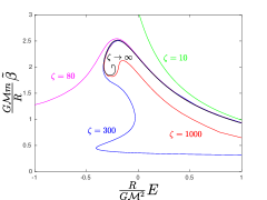
(a) Low energy.

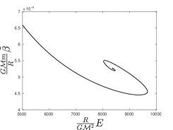
(b) High energy.

Figure 1: Caloric curves for rest mass compactness $\xi=0.01$ and various values of the system size $\zeta$. The number of particles and the size of the system are fixed. This value of $\xi$ corresponds to $R\gg R_{S}$ suggesting that the system is in the Newtonian gravity limit. We denote $E$ the energy of the system subtracted by the total rest mass $E=Mc^{2}-\mathcal{M}c^{2}$. Left: The black spiral curve corresponds to the classical limit $\zeta\rightarrow\infty$. Every curve ends to the right with an anti-clockwise spiral, shown in the right panel, that denotes a relativistic gravothermal instability. The curve $\zeta=80$ continues indefinitely (though not shown here) towards zero temperature ($\tilde{\beta}\rightarrow+\infty$) tending asymptotically to a minimum energy $E_{\rm min}$ like in Figure 5(a). The curve $\zeta=300$ designates equilibria with a condensed nearly degenerate core and, although the chosen value of $\xi$ implies $R\gg R_{S}$, the core radius satisfies $R_{\rm C}\sim R_{S}$, as may be inferred from Figure 4. It undergoes a relativistic instability at sufficiently low energy when the core is sufficiently condensed (such that $N_{C}>N_{\rm OV}$). Right: This spiral designates the high-energy gravothermal instability [1, 22]. The self-gravitating gas collapses under the weight of its own thermal energy. For this value of $\xi$, the value of $\zeta$ does not alter significantly the turning point of stability, but at relativistic $\xi$ values, the $\zeta$ value does affect this instability, as shown in Figure 6.

(a) Inverse temperature

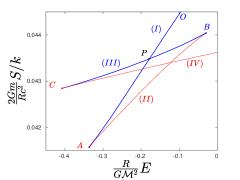
(b) Entropy

Figure 2: $\xi=0.01$, $\zeta=300$. Blue, thick branches $(I)$ and $(III)$ are stable, while red, thin branches $(II)$ and $(IV)$ are unstable in the microcanonical ensemble. The stability of the solutions can be deduced from the Poincaré turning point criterion [42]. Branch $(I)$ is in the gaseous phase while branch $(III)$ is in the condensed phase. Point $P$ designates a first order phase transition from configuration $P_{1}$ to $P_{2}$ (it can be determined from the Maxwell construction or from the equality of the entropy of the two phases). We note that the first order phase transition does not take place in practice because of the very long lifetime of metastable states, scaling as $e^{N}$, for systems with long-range interactions [17]. Therefore, the physical phase transition is the zeroth order phase transition which takes place at the spinodal point $A$ where the metastable gaseous phase disappears (gravothermal catastrophe). At point $C$ a relativistic instability sets in to the nearly degenerate, condensed core, which collapses further when the number of particles that it contains passes above the OV limit.

There appear two marginal values $\zeta_{\rm MCP}=154$ and $\zeta_{c}=396$ of the system size. For $\zeta<\zeta_{\rm MCP}=154$ the gravothermal catastrophe is suppressed and does not occur as in the cases $\zeta=10,80$ of Figure 1. For $\zeta_{\rm MCP}=154<\zeta<\zeta_{c}=396$ the gravothermal catastrophe does occur at $E_{A}$, but it is halted by a degenerate configuration, as in the case $\zeta=300$ in Figures 1 and 2. In this case a gravitational phase transition takes place from the gaseous phase to the condensed phase. However, this (nearly) degenerate configuration undergoes a new type of instability on its turn at $E_{C}$. This happens when the number of particles $N_{C}$ in the core passes above the OV limit $N_{\rm OV}$ leading to core collapse. The turning point of this instability is denoted by the letter $C$ in Figure 2(a), while letter $A$ denotes the gravothermal catastrophe. The density and temperature distributions of the two phases, core-halo phase and gaseous phase, are given in Figure 3. For $\zeta>\zeta_{c}=396$ the gravothermal catastrophe not only occurs but collapse at $E_{A}$ cannot be halted because $E_{C}>E_{A}$ or because every condensed configuration is unstable as in the case $\zeta=1000$ of Figure 1 (the condensed phase disappears or becomes unstable for $\zeta>\zeta^{\prime}_{*}$ slightly larger than $\zeta_{c}$).

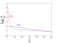
(a) Density

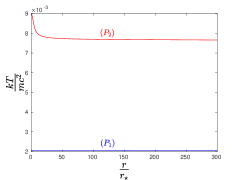
(b) Temperature

Figure 3: $\xi=0.01$, $\zeta=300$. The density and temperature profiles for the gaseous phase $(P_{1})$, which corresponds to point $P_{1}$ of Figure 2(a), and the condensed phase $(P_{2})$, which corresponds to point $P_{2}$ of Figure 2(a). Clearly $(P_{2})$ consists of an ultra-dense core and a diluted halo, while $(P_{1})$ is comparatively nearly homogeneous. The condensed phase occurs at higher temperature than the gaseous phase and the core is substantially hotter than the halo with a significant Tolman-Ehrenfest effect taking place. In contrast, the temperature of the gaseous phase is nearly homogeneous. This is because the gaseous phase is weakly relativistic while the condensed phase is strongly relativistic. Both configurations have common entropy corresponding to point $P$ of Figure 2(b).

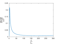
(a) Compactness

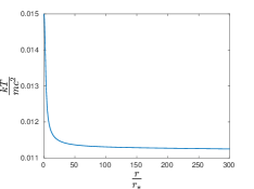
(b) Temperature

Figure 4: $\xi=0.01$, $\zeta=300$. The compactness and temperature profiles of the equilibrium at point $C$ of Figure 2(a), where a relativistic instability sets in. Although for the whole sphere the compactness $2GM/Rc^{2}\simeq 2G\mathcal{M}/Rc^{2}=0.01$ is small, the Newtonian approximation is not valid because the system has developed a very relativistic dense core ($R_{C}\ll R$) for which $2GM_{C}/R_{C}c^{2}\simeq 0.22$, leading to a general relativistic instability.

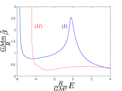
(a) Inverse temperature

(b) Entropy

Figure 5: $\xi=0.01$, $\zeta=80$. Above $\zeta_{1}=40.8$ appear two distinct series of equilibria. Blue, thick branch $(I)$ is stable and has a higher entropy than the red thin unstable branch $(II)$. It is the analogue of branch $(IV)$ of Figure 2(a), but separated. The branches present two vertical asymptotes at $E_{\rm min}$ and $E^{\prime}_{\rm min}$ where $\tilde{\beta}\rightarrow+\infty$. They correspond to the stable and first unstable equilibrium states of the general relativistic Fermi gas at $T=0$. The two series of equilibria merge at $\zeta_{\rm OV}=90.0$ where the asymptotes disappear.

The series of equilibria are intersecting in various cases as in Figures 2(a) and 5(a). This does not a raise a problem, because what is plotted is the Tolman temperature. So there is a third parameter (apart from the energy and the Tolman temperature) that defines each configuration. This is the central temperature $b_{0}$. Therefore at the point of intersection there correspond two distinct equilibria with the same Tolman temperature and energy but with different central temperature. As already implied, the equilibrium in the condensed phase has a much larger central temperature so that the core is much hotter than the center region of the corresponding gaseous phase that does not posses a core. Note, however, that as we explained earlier the temperature normalized to the corresponding Fermi temperature is smaller for the core than the gaseous phase. Only one of these two configurations is stable. The condensed configurations on branch (IV) in Figure 2(a) and on branch (II) in Figure 5(a) are unstable while the gaseous configurations on branch (I) in Figures 2(a) and 5(a) are stable.

In Figure 6 are drawn the caloric curves for $\xi=0.25$ and various $\zeta=0.5,\;1,\;10$ (here $\zeta_{\rm min}=0.185$). This value of $\xi$ corresponds to a very strong gravitational field where general relativity cannot be ignored at any case. For this value of $\xi$ the phase transitions are suppressed for any $\zeta$. For $\zeta<\zeta_{\rm OV}=3.60$ the first branch presents an asymptote at $E_{\rm min}$ where $\tilde{\beta}\rightarrow+\infty$. A second branch with an asymptote at $E^{\prime}_{\rm min}$ appears at $\zeta_{1}=1.45$ (this branch is unstable, similar to branch (II) in Figure 5(a), and is not presented). The first and second branches (i.e. the asymptotes at $E_{\rm min}$ and $E^{\prime}_{\rm min}$) merge at $\zeta_{\rm OV}=3.60$.

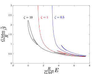
Figure 6: $\xi=0.25$. This value of $\xi$ corresponds to a very strong gravitational field. The phase transition to a condensed phase is suppressed. There are only two possibilities depending on the value of the system’s size $\zeta$: the appearance of the low energy gravothermal instability when $\zeta>\zeta_{\rm OV}=3.60$ or the complete suppression of it and the existence of equilibria until $\tilde{T}=0$ and $E_{\rm min}$ (ground state) when $\zeta<\zeta_{\rm OV}=3.60$. At sufficient high energy there appears the high-energy gravothermal instability [1, 22] for any value of compactness and size.

5 Summary and conclusion

We have provided an illustration of microcanonical phase transitions and instabilities in the general relativistic Fermi gas at nonzero temperature. We have specified a value of the rest mass compactness $\xi=2G{\cal M}/Rc^{2}$ and studied the caloric curves as a function of the system size $\zeta=R/r_{*}$. We have first considered a low value of the rest mass compactness, $\xi=0.01$, so that our system is expected to be close to the Newtonian gravity limit. For $\zeta<\zeta_{\rm MCP}$ there is no phase transition but a region of negative specific heat appears for $\zeta>\zeta_{\rm CCP}$. For $\zeta>\zeta_{\rm MCP}$ the system undergoes a gravothermal catastrophe at some critical relativistic Antonov energy $E_{A}$. For $\zeta_{\rm MCP}<\zeta<\zeta_{c}$ the gravothermal catastrophe is halted by quantum degeneracy (Pauli’s exclusion principle) so that a microcanonical phase transition from a gaseous phase to a condensed phase occurs. However, at a lower energy $E_{C}$, the condensed phase undergoes a relativistic instability which occurs for $\zeta>\zeta_{\rm OV}$. This is because the condensed phase has a core-halo structure and the degenerate core becomes relativistically unstable. For $\zeta>\zeta_{c}$, we find that quantum mechanics cannot arrest the gravothermal catastrophe at $E_{A}$ so that the gaseous phase collapses without passing through a condensed state. We have then considered a higher value of the rest mass compactness, $\xi=0.25$, corresponding to a strongly relativistic regime. In that case, there is no phase transition. However, a low-energy gravothermal instability occurs for $\zeta>\zeta_{\rm OV}$. The high-energy gravothermal instability appears for any values of the control parameters $\xi$, $\zeta$. This is evidence of its universal character [22].

Appendix A Domains of validity of the different regimes

In this Appendix, we determine the domains of validity of the different regimes as a function of $\xi$ and $\zeta$ using the general results from [35].

A.1 The general relativistic Fermi gas at $T=0$

Figure 7: Particle number-radius relation for the general relativistic Fermi gas at $T=0$.

We first consider the general relativistic Fermi gas at $T=0$. This model was originally studied by Oppenheimer and Volkoff [29] in the context of neutron stars. In that case, the system is self-confined and the material box is not necessary. The particle number-radius relation is plotted in Fig. 7. It has a snail-like (spiral) structure. There is no equilibrium state above a maximum particle number

$$N_{\rm OV}=0.39853\,\sqrt{\frac{2}{g}}\left(\frac{\hbar c}{G}\right)^{3/2}\frac{1}{m^{3}}=0.449693\,N_{\star}.$$ (55)

The corresponding maximum mass and minimum radius are

$$M_{\rm OV}=0.38426\,\sqrt{\frac{2}{g}}\left(\frac{\hbar c}{G}\right)^{3/2}\frac{1}{m^{2}}=0.433591\,M_{\star},$$ (56)

$$R_{\rm OV}=8.7360\,\frac{GM_{\rm OV}}{c^{2}}=3.3569\,\sqrt{\frac{2}{g}}\left(\frac{\hbar^{3}}{Gc}\right)^{1/2}\frac{1}{m^{2}}=3.78786\,r_{\star}.$$ (57)

For $N<N_{1}$, where

$$N_{1}=0.18131\,\sqrt{\frac{2}{g}}\left(\frac{\hbar c}{G}\right)^{3/2}\frac{1}{m^{3}}=0.20459\,N_{\star},$$ (58)

with corresponding mass and radius

$$M_{1}=0.19893\,\sqrt{\frac{2}{g}}\left(\frac{\hbar c}{G}\right)^{3/2}\frac{1}{m^{2}}=0.22447\,M_{\star},$$ (59)

$$R_{1}=2.0556\,\sqrt{\frac{2}{g}}\left(\frac{\hbar^{3}}{Gc}\right)^{1/2}\frac{1}{m^{2}}=2.3195\,r_{\star},$$ (60)

there is only one equilibrium state at $T=0$ and it is stable. For $N_{1}<N<N_{\rm OV}$ there are two or more (up to an infinity) equilibrium states at $T=0$. However, only the equilibrium states on the main branch, before the first turning point of $N(\epsilon_{0})$ at $N_{\rm max}$, are stable (this corresponds to a mass-radius ratio less than $(2GM/Rc^{2})_{\rm max}=0.229$). The other equilibrium states are unstable and they have more and more modes of instability as the $N(R)$ curve spirals inwards. Below, we shall consider only the first unstable equilibrium state. It appears suddenly at $N_{1}$ (as we increase $N$) and merges with the stable equilibrium state at $N_{\rm OV}$.

This observation allows us to understand one important feature of the caloric curves of the general relativistic Fermi gas. For $N<N_{\rm OV}$ there exists a stable equilibrium state at $T=0$. This is the limit point of the main branch of the caloric curve ending on an asymptote at $E_{\rm min}$ and $\tilde{\beta}=+\infty$ (ground state). For $N_{1}<N<N_{\rm OV}$ there exists in addition an unstable equilibrium state at $T=0$. This is the limit point of the secondary branch of the caloric curve ending on an asymptote at $E^{\prime}_{\rm min}$ and $\tilde{\beta}=+\infty$ (at $N=N_{1}$ we have $E^{\prime}_{\rm min}R/G{\cal M}^{2}=0.53617R$ and $E_{\rm min}R/G{\cal M}^{2}=-0.0570R$). The two branches merge at $N_{\rm OV}$ where the asymptotes at $E_{\rm min}$ and $E^{\prime}_{\rm min}$ meet each other (at $N=N_{\rm OV}$ we have $E^{\prime}_{\rm min}R/G{\cal M}^{2}=E_{\rm min}R/G{\cal M}^{2}=-0.08985R$). For $N>N_{\rm OV}$ there is no ground state, i.e., there is no stable equilibrium state at $T=0$ anymore. As a result, there is no vertical asymptote in the caloric curve. In that case, the system undergoes gravitational collapse below a critical temperature or below a critical energy. They correspond to turning points of temperature $\tilde{T}(\epsilon_{0})$ and energy $E(\epsilon_{0})$ in the series of equilibria.

A.2 The phase diagram of the nonrelativistic Fermi gas

In the nonrelativistic limit, the caloric curve of the self-gravitating Fermi gas depends on a single control parameter (instead of depending on $N$ and $R$ individually) which can be written as [17]:

$$\mu=\sqrt{2\frac{N}{N_{\star}}\frac{R^{3}}{r_{\star}^{3}}}.$$ (61)

The phase diagram of the nonrelativistic self-gravitating Fermi gas is given in [17]. It is shown in this paper that a canonical phase transition appears above $\mu_{\rm CCP}=83$ and that a microcanonical phase transition appears above $\mu_{\rm MCP}=2670$. For a given radius $R$, using equation (61), we conclude that the canonical phase transition appears above the particle number

$$\frac{N^{\rm NR}_{\rm CCP}(R)}{N_{*}}=3.44\times 10^{3}\left(\frac{r_{*}}{R}\right)^{3},$$ (62)

and that the microcanonical phase transition appears above the particle number

$$\frac{N^{\rm NR}_{\rm MCP}(R)}{N_{*}}=3.57\times 10^{6}\left(\frac{r_{*}}{R}\right)^{3}.$$ (63)

A.3 The phase diagram of the general relativistic Fermi gas in the $(R,N)$ plane

In the general relativistic case, the caloric curves of the self-gravitating Fermi gas depend on $R$ and $N$ individually. The phase diagram of the general relativistic Fermi gas in the $(R,N)$ plane has been obtained in [35]. It is reproduced in Figure 8 with the notations of the present paper. We recall below the meaning of the different curves (we refer to [35] for a more detailed description):

(i) The curve $N_{1}(R)$ signals the appearance of a second branch of solutions in the caloric curve (corresponding to unstable equilibrium states). For $R/r_{*}>R_{1}/r_{*}=2.32$, we have $N_{1}/N_{*}=0.204$. For $R/r_{*}\ll R_{1}/r_{*}=2.32$, we have $N_{1}(R)/N_{*}\sim 0.234(R/r_{*})^{3/2}$.

(ii) The curve $N_{\rm OV}(R)$ signals the disappearance of the ground state (i.e. there is no equilibrium state at $T=0$ anymore). At that point, the asymptotes at $E_{\rm min}$ and $E^{\prime}_{\rm min}$ of the first and second branches in the caloric curve merge, then disappear. For $R/r_{*}>R_{\rm OV}/r_{*}=3.79$, we have $N_{\rm OV}/N_{*}=0.450$. For $R/r_{*}\ll R_{\rm OV}/r_{*}=3.79$, we have $N_{\rm OV}(R)/N_{*}\sim 0.292(R/r_{*})^{3/2}$.

(iii) The curve $N_{\rm max}(R)$ is the maximum particle number for which there are equilibrium states. For $R/r_{*}\gg R_{\rm OV}/r_{*}=3.79$, we have $N_{\rm max}(R)/N_{*}=0.1764R/r_{*}$. For $R/r_{*}\ll R_{\rm OV}/r_{*}=3.79$, we have $N_{\rm max}(R)/N_{*}\sim 0.292(R/r_{*})^{3/2}$.

(iv) There is no canonical phase transition when $R/r_{*}<R_{\rm CCP}/r_{*}=13.5$. When $R/r_{*}>R_{\rm CCP}/r_{*}=13.5$, the curve $N_{\rm CCP}(R)$ signals the appearance of a canonical phase transition. For $R/r_{*}\gg R_{\rm CCP}/r_{*}=13.5$, we have $N_{\rm CCP}/N_{*}\sim 3.44\times 10^{3}(r_{*}/R)^{3}$. The curve $N_{*}(R)$ signals the disappearance of the condensed phase in the canonical ensemble. Note that $N_{*}(R)$ is very close to the value $N_{c}^{\rm CE}(R)$ at which the isothermal collapse is not halted by quantum mechanics.

(v) There is no microcanonical phase transition when $R/r_{*}<R_{\rm MCP}/r_{*}=104$. When $R/r_{*}>R_{\rm MCP}/r_{*}=104$, the curve $N_{\rm MCP}(R)$ signals the appearance of a microcanonical phase transition. For $R/r_{*}\gg R_{\rm MCP}/r_{*}=104$, we have $N_{\rm MCP}/N_{*}\sim 3.57\times 10^{6}(r_{*}/R)^{3}$. The curve $N_{*}^{\prime}(R)$ signals the disappearance of the condensed phase in the microcanonical ensemble. Note that $N_{*}^{\prime}(R)$ is very close to the value $N_{c}^{\rm MCE}(R)$ at which the gravothermal catastrophe is not halted by quantum mechanics.

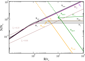
Figure 8: The phase diagram of the general relativistic Fermi gas in the $(R,N)$ plane (taken from [35]).

A.4 The $(\xi,\zeta)$ variables

In the present paper, we have taken the rest mass compactness

$$\xi=\frac{2GNm}{Rc^{2}}=\frac{2N/N_{\star}}{R/r_{\star}}$$ (64)

and the box radius

$$\zeta=\frac{R}{r_{\star}}$$ (65)

as control parameters. We shall fix the relativistic parameter $\xi$ and describe the caloric curves and the phase transitions as a function of the box radius $\zeta$, using the phase diagram of Fig. 8. We note that fixing $\xi$ determines a straight line of equation $N/N_{\star}=(\xi/2)(R/r_{\star})$ in the phase diagram of Fig. 8. Therefore, changing $\zeta$ at fixed $\xi$ amounts to moving along that line. For a fixed value of $\xi$, we find that:

(i) There is no equilibrium state above $\xi_{\rm max}=0.353$, whatever the value of the energy and of the temperature.

(ii) The smallest possible value of $\zeta$ is $\zeta_{\rm min}(\xi)$. For $\xi\ll\xi_{\rm max}=0.353$ we have $\zeta_{\rm min}(\xi)\sim 2.93\xi^{2}$.

(ii) The second branch in the caloric curve appears at $\zeta_{1}(\xi)$. For $\xi\ll\xi_{\rm max}=0.353$ we have $\zeta_{1}(\xi)\sim 0.408/\xi$.

(iii) The ground state (equilibrium state at $T=0$) disappears at $\zeta_{\rm OV}(\xi)$. At that point, the asymptotes at $E_{\rm min}$ and $E^{\prime}_{\rm min}$ of the first and second branches merge, then disappear. For $\xi\ll\xi_{\rm max}=0.353$ we have $\zeta_{\rm OV}(\xi)\sim 0.900/\xi$.

(iv) There is no canonical phase transition when $\xi>\xi_{\rm CCP}=0.0707$. When $\xi<\xi_{\rm CCP}=0.0707$, the canonical phase transition appears at $\zeta_{\rm CCP}(\xi)$. When $\xi\ll\xi_{\rm CCP}=0.0707$, we have $\zeta^{\rm NR}_{\rm CCP}(\xi)=9.11/\xi^{1/4}$. The canonical phase transition disappears at $\zeta_{*}(\xi)$. Note that $\zeta_{*}(\xi)$ is very close to the value $\zeta_{c}^{\rm CE}(\xi)$ at which the isothermal collapse is not halted by quantum mechanics.

(v) There is no microcanonical phase transition when $\xi>\xi_{\rm MCP}=0.0272$. When $\xi<\xi_{\rm MCP}=0.0272$, the microcanonical phase transition appears at $\zeta_{\rm MCP}(\xi)$. When $\xi\ll\xi_{\rm MCP}=0.0272$, we have $\zeta^{\rm NR}_{\rm MCP}(\xi)=51.7/\xi^{1/4}$. The microcanonical phase transition disappears at $\zeta^{\prime}_{*}(\xi)$. Note that $\zeta^{\prime}_{*}(\xi)$ is very close to the value $\zeta_{c}^{\rm MCE}(\xi)$ at which the gravothermal catastrophe is not halted by quantum mechanics. Two situations may occur. Let us first assume $\xi<\xi^{\prime}_{\rm MCP}=0.00461$. In that case: when $\zeta_{\rm MCP}(\xi)<\zeta<\zeta_{\rm OV}(\xi)$ the condensed phase is stable for all energies because $N<N_{\rm OV}$; when $\zeta_{\rm OV}(\xi)<\zeta<\zeta^{\prime}_{*}(\xi)$ the condensed phase collapses at small energies because $N>N_{\rm OV}$. Let us now assume $\xi^{\prime}_{\rm MCP}=0.00461<\xi<\xi_{\rm MCP}=0.0272$. In that case, the condensed phase collapses at small energies because $N>N_{\rm OV}$.

In this paper, for illustration, we have considered two specific values of $\xi$.

For $\xi=0.01$, we plot on Fig. 8 the straight line $N/N_{\star}=0.005R/r_{\star}$. We have $\zeta_{\rm min}=2.93\times 10^{-4}$. The second branch appears at $\zeta_{1}=40.8$. The first and second branches merge at $\zeta_{\rm OV}=90.0$. The canonical phase transition appears at $\zeta_{\rm CCP}=28.7$ and ends at $\zeta_{*}=93.5$. The microcanonical phase transition appears at $\zeta_{\rm MCP}=154$ and ends at $\zeta^{\prime}_{*}=395.7$.

For $\xi=0.25$, we plot on Fig. 8 the straight line $N/N_{\star}=0.125R/r_{\star}$. We have $\zeta_{\rm min}=0.185$. The second branch appears for $\zeta_{1}=1.45$. The first and second branches merge at $\zeta_{\rm OV}=3.60$. There is no canonical and no microcanonical phase transition.

A.5 Validity of the nonrelativistic and classical limits

As discussed in detail in [35], the nonrelativistic limit corresponds to $R\rightarrow+\infty$ and $N\rightarrow 0$ (physically $R\gg R_{\rm OV}$ and $N\ll N_{\rm OV}$) with $NR^{3}$ fixed. This corresponds to the lower right panel of Fig. 8. In terms of the variables ($\xi,\zeta$), for a given value of $\xi\ll\xi_{\rm max}$, this corresponds to $1\ll\zeta\ll\zeta_{\rm OV}(\xi)$ and $\zeta\gg\zeta_{c}(\xi)$ (these two distinct regions are explained in Sec. XI of [35]). On the other hand, the classical limit corresponds to $R\rightarrow+\infty$ and $N\rightarrow+\infty$ (physically $R\gg R_{\rm OV}$ and $N\gg N_{\rm OV}$) with $N/R$ fixed. This corresponds to the upper right panel of Fig. 8. In terms of the variables ($\xi,\zeta$), for a given value of $\xi<\xi_{\rm max}$, this corresponds to $\zeta\gg\zeta_{\rm OV}(\xi)$.

References

References

- [1] Z. Roupas. Relativistic gravothermal instabilities. Class. Quant. Grav., 32(13):135023, 2015.
- [2] V. A. Antonov. Solution of the problem of stability of stellar system with Emden’s density law and the spherical distribution of velocities. Vestnik Leningradskogo Universiteta, Leningrad: University, 1962.
- [3] D. Lynden-Bell and R. Wood. The gravo-thermal catastrophe in isothermal spheres and the onset of red-giant structure for stellar systems. MNRAS, 138:495, 1968.
- [4] R. Emden. Gaskugeln. Teubner Verlag, Leipzig, 1907.
- [5] S. Chandrasekhar. An introduction to the study of stellar structure. Chicago, iLLINOIS, 1938.
- [6] J. Katz. On the number of unstable modes of an equilibrium. MNRAS, 183:765–770, June 1978.
- [7] G. Horwitz and J. Katz. Steepest descent technique and stellar equilibrium statistical mechanics. III Stability of various ensembles. ApJ, 222:941–958, June 1978.
- [8] A. Campa, T. Dauxois, D. Fanelli, and S. Ruffo. Physics of Long-Range Interacting Systems. Oxford University Press, 2014.
- [9] Terell L. Hill. Statistical Mechanics: Principles and Selected Applications. Dover Publications inc., 1956.
- [10] T. Padmanabhan. Antonov instability and gravothermal catastrophe - Revisited. Astrophys. J. Supp., 71:651–664, November 1989.
- [11] P. H. Chavanis. Gravitational instability of finite isothermal spheres. Astron. Astrophys., 381:340–356, January 2002.
- [12] P. H. Chavanis. Gravitational instability of isothermal and polytropic spheres. Astron. Astrophys., 401:15–42, April 2003.
- [13] H. J. de Vega and N. Sánchez. Statistical mechanics of the self-gravitating gas: I. Thermodynamic limit and phase diagrams. Nuclear Physics B, 625:409–459, March 2002.
- [14] H. J. de Vega and N. Sánchez. Statistical mechanics of the self-gravitating gas: II. Local physical magnitudes and fractal structures. Nuclear Physics B, 625:460–494, March 2002.
- [15] T. Padmanabhan. Statistical mechanics of gravitating systems. Phys. Rep. , 188:285–362, April 1990.
- [16] J. Katz. Thermodynamics and Self-Gravitating Systems. Found. Phys., 33:223–269, 2003.
- [17] P. H. Chavanis. Phase Transitions in Self-Gravitating Systems. International Journal of Modern Physics B, 20:3113–3198, 2006.
- [18] R. D. Sorkin, R. M. Wald, and Z. Z. Jiu. Entropy of self-gravitating radiation. General Relativity and Gravitation, 13(12):1127–1146, 1981.
- [19] P. H. Chavanis. Gravitational instability of finite isothermal spheres in general relativity. Analogy with neutron stars. Astron. Astrophys., 381:709–730, January 2002.
- [20] P. H. Chavanis. Relativistic stars with a linear equation of state: analogy with classical isothermal spheres and black holes. Astron. Astrophys., 483:673–698, June 2008.
- [21] Z. Roupas. Thermodynamical instabilities of perfect fluid spheres in General Relativity. Classical and Quantum Gravity, 30(11):115018, June 2013.
- [22] Z. Roupas. Relativistic gravothermal instability: the Weight of Heat. arXiv:1809.04408, September 2018.
- [23] P. Hertel and W. Thirring. Free energy of gravitating fermions. Communications in Mathematical Physics, 24:22–36, March 1971.
- [24] N. Bilić and R. D. Viollier. Gravitational phase transition of fermionic matter. Physics Letters B, 408:75–80, February 1997.
- [25] R. H. Fowler. On dense matter. MNRAS, 87:114–122, December 1926.
- [26] E.C. Stoner. Phil. Mag., 7:63, 1929.
- [27] E. A. Milne. The analysis of stellar structure. MNRAS, 91:4–55, November 1930.
- [28] S. Chandrasekhar. Xlviii. the density of white dwarf stars. The London, Edinburgh, and Dublin Philosophical Magazine and Journal of Science, 11(70):592–596, 1931.
- [29] J. R. Oppenheimer and G. M. Volkoff. On Massive Neutron Cores. Physical Review, 55:374–381, February 1939.
- [30] Z. Roupas. Thermal mass limit of neutron cores. Phys. Rev. D, 91(2):023001, January 2015.
- [31] Adam Burrows and James M. Lattimer. The birth of neutron stars. Astrophys.J., 307:178–196, 1986.
- [32] Madappa Prakash, Ignazio Bombacia, Manju Prakasha, Paul J. Ellisb, James M. Lattimerd, and Roland Knorren. Composition and structure of protoneutron stars. Physics Reports, 280:1–77, 1997.
- [33] J. M. Lattimer and M. Prakash. The equation of state of hot, dense matter and neutron stars. Phys. Rep. , 621:127–164, March 2016.
- [34] N. Bilić and R. D. Viollier. Gravitational phase transition of fermionic matter in a general-relativistic framework. European Physical Journal C, 11:173–180, November 1999.
- [35] G. Alberti and P.-H. Chavanis. Caloric curves of self-gravitating fermions in general relativity. arXiv:1808.01007, August 2018.
- [36] P. T. Landsberg and J. Dunning-Davies. Statistical thermodynamics of the ideal relativistic quantum gas. In J. Meixner, editor, Statistical Mechanics of Equilibrium and Non-equilibrium, page 36, 1965.
- [37] J. P. Cox and R. T. Giuli. Principles of stellar structure . 1968.
- [38] S. Weinberg. Gravitation and Cosmology: Principles and Applications of the General Theory of Relativity. July 1972.
- [39] Richard C. Tolman. On the weight of heat and thermal equilibrium in general relativity. Phys. Rev., 35:904, 1930.
- [40] Richard C. Tolman and Paul Ehrenfest. Temperature equilibrium in a static gravitational field. Phys. Rev., 36:1791–1798, 1930.
- [41] Z. Roupas. Corrigendum: Thermodynamical instabilities of perfect fluid spheres in General Relativity. Classical and Quantum Gravity, 32(11):119501, June 2015.
- [42] H. Poincaré. Sur l’équilibre d’une masse fluide animée d’un mouvement de rotation. Acta. Math., 7:259, 1885.