Where are the double-degenerate progenitors of type Ia supernovae?

Abstract

Double white dwarf binaries with merger timescales smaller than the Hubble time and with a total mass near the Chandrasekhar limit (i.e. classical Chandrasekhar population) or with high-mass primaries (i.e. sub-Chandrasekhar population) are potential supernova type Ia (SNIa) progenitors. However, we have not yet unambiguously confirmed the existence of these objects observationally, a fact that has been often used to criticise the relevance of double white dwarfs for producing SNIa. We analyse whether this lack of detections is due to observational effects. To that end we simulate the double white dwarf binary population in the Galaxy and obtain synthetic spectra for the SNIa progenitors. We demonstrate that their identification, based on the detection of H$\alpha$ double-lined profiles arising from the two white dwarfs in the synthetic spectra, is extremely challenging due to their intrinsic faintness. This translates into an observational probability of finding double white dwarf SNIa progenitors in the Galaxy of $(2.1\pm 1.0)\times 10^{-5}$ and $(0.8\pm 0.4)\times 10^{-5}$ for the classical Chandrasekhar and the sub-Chandrasekhar progenitor populations, respectively. Eclipsing double white dwarf SNIa progenitors are found to suffer from the same observational effect. The next generation of large-aperture telescopes are expected to help in increasing the probability for detection by $\sim$1 order of magnitude. However, it is only with forthcoming observations such as those provided by LISA that we expect to unambiguously confirm or disprove the existence of double white dwarf SNIa progenitors and to test their importance for producing SNIa.

1 Introduction

Supernovae Type Ia (SNIa) are one of the most luminous events in the Universe, which makes them ideal tools for cosmological studies since they can be detected at very large distances. In particular, SNIa have been used to prove the accelerated expansion of the Universe, a discovery which was awarded the Nobel prize in physics in 2011 (e.g. Riess et al., 1998; Perlmutter et al., 1999; Astier & Pain, 2012). However, there is not yet a consensus on the leading paths to SNIa (see Livio & Mazzali, 2018; Soker, 2018; Wang, 2018, for recent reviews). This progenitor uncertainty may introduce some not yet known systematic errors in the determination of extragalactic distances, thus compromising the use of SNIa as standard candles (Linden et al., 2009; Howell, 2011).

Several evolutionary channels have been proposed that lead to a SNIa explosion. For a comprehensive review, see Livio & Mazzali (2018); Wang (2018). Among these, the two classical scenarios are the single- and the double-degenerate channels. In the single-degenerate channel a WD in a binary system accretes mass from a non-degenerate donor until it grows near the Chandrasekhar limit (Whelan & Iben, 1973; Han & Podsiadlowski, 2004; Nomoto & Leung, 2018). In the double-degenerate channel two WDs in a close binary system merge due to angular momentum loss caused by the emission of gravitational waves and the resulting merger has a mass near the Chandrasekhar limit (Whelan & Iben, 1973; Iben & Tutukov, 1984; Liu et al., 2018). Additional evolutionary channels for SNIa include the double-detonation mechanism (Woosley & Weaver, 1986; Livne & Arnett, 1995; Shen et al., 2012), the violent merger model (Pakmor et al., 2010; Sato et al., 2016), the core-degenerate channel (Sparks & Stecher, 1974; Livio & Riess, 2003; Kashi & Soker, 2011; Wang et al., 2017) and a mechanism which involves the collision of two WDs (Benz et al., 1989; Kushnir et al., 2013; Aznar-Siguán et al., 2013). In the double-detonation scenario a WD accumulates helium-rich material on its surface, which is compressed and ultimately detonates. The compression wave propagates towards the center of the WD and a second detonation occurs near the center of its carbon-oxygen core. In the violent merger model, the detonation of the white dwarf core is initiated during the early stages of the merger. This can happen, for example, due to compressional heating by accretion from the disrupted secondary or due to a preceeding detonation of accreted helium (alike the double-detonation scenario) that is ignited dynamically (Pakmor et al., 2010, 2011, 2012, 2013; Guillochon et al., 2010; Kashyap et al., 2015; Sato et al., 2015, 2016). In the core-degenerate scenario a WD merges with the hot core of an asymptotic giant branch star during (or after) a common envelope phase. Finally, the evolutionary phase involving the collision of two WDs requires a tertiary star which brings the two WDs to collide due to the Kozai-Lidov mechanism, or dynamical interactions in a dense stellar system, where this kind of interaction is more likely to happen.

The viability of the above described SNIa formation channels has been intensively studied during the last several years both theoretically and observationally – see, for example, the reviews by Hillebrandt et al. (2013); Maoz et al. (2014); Wang (2018); Soker (2018) and references therein. However, there is not yet an agreement on how these different evolutionary paths contribute to the observed population of SNIa, with all channels presenting advantages and drawbacks. In particular, from the theoretical perspective, it is not clear whether double WD mergers arising from the double-degenerate channel result in a SNIa explosion or rather in an accretion-induced collapse to a neutron star (Nomoto & Iben, 1985; Shen et al., 2012). The hypothesis that WD mergers containing less massive primaries, i.e. the so called sub-Chandrasekhar WDs, play a decisive role in reproducing the observed SNIa luminosity function is also under debate (e.g. Shen et al., 2017). It is also fair to mention that double-degenerate models predict a delay time distribution which is in better agreement with the one derived from observations (e.g. Maoz & Graur, 2017). Furthermore, several additional observational analyses have provided support for the double-degenerate channel (Tovmassian et al., 2010; Rodríguez-Gil et al., 2010; González Hernández et al., 2012; Olling et al., 2015). However, perhaps with the exception of the central binary system of the planetary nebula Henize 2-428 (Santander-García et al., 2015), there is no single system yet that has robustly been confirmed as a double-degenerate SN Ia progenitor. The nature of Henize 2-428 as a direct SNIa double-degenerate progenitor has been criticised by García-Berro et al. (2016), who claim that the binary system may be formed by a WD and a low-mass main sequence companion, or two WDs of smaller combined mass than that estimated by Santander-García et al. (2015).

Finding close double-degenerate binaries is not straightforward since their spectra are virtually identical to those of single WDs. Hence, their identification has been mainly based on the detection of radial velocity variations (Marsh et al., 1995; Maxted et al., 2000, 2002; Maxted & Marsh, 1999; Brown et al., 2013, 2016; Kilic et al., 2017; Rebassa-Mansergas et al., 2017). In particular, the observational effort carried out by the ESO SNIa Progenitor (SPY) Survey (Napiwotzki et al., 2001, 2007) has provided radial velocities for hundreds of double WDs, including the identification of several double-lined binaries (Koester et al., 2001). More recently, Breedt et al. (2017) analysed multiple spectra available for individual WDs in the SDSS to preselect targets displaying variability for follow-up observations. Although no direct SNIa progenitors has been identified, the analysis of both samples (SPY and SDSS) have allowed constraining the binary fraction, merger rate and separation distributions of double WDs in the Galaxy (Maoz et al., 2012; Badenes & Maoz, 2012; Maoz et al., 2018) as well as identifying hot sub-dwarf plus white dwarf binaries (Geier et al., 2010) and white dwarf plus M dwarf binaries (Rebassa-Mansergas et al., 2011, 2016).

The fact that not a single double-degenerate progenitor has been unambiguously identified among our currently available large samples of double WDs may be used as an argument indicative of the double-degenerate mechanism not being a viable channel for SNIa. However, it is also fair to mention that identifying SNIa progenitors not only requires measuring the orbital periods but also the component masses of the two WDs. Even with such large superb samples of double WDs at hand, only few of them have well measured component masses (see Rebassa-Mansergas et al., 2017, and reference therein). The obvious question is then: what is the probability of identifying SNIa double-degenerate progenitors? Or in other words: are we not identifying double-degenerate progenitors because it is observationally challenging or because they simply do not exist? We assess these questions quantitatively in this paper. To that end we simulate the close double WD population in the Galaxy and we analyse whether or not the SNIa progenitors in our simulations would be easily identified observationally with our current telescopes and instrumentation.

Table 1: The total number of double WDs in the four populations considered in this work. The numbers vary according to the common envelope prescription adopted in the simulations. Note that our simulations exclude all binaries in which any of the WD components has a $g$ magnitude $>23$ mag.

CE formalism	Ch. direct	SCh. direct	Ch. nmer	SCh. nmer
$\alpha\alpha$	176	51	14065	7431
$\gamma\alpha$	107	22	21596	8476

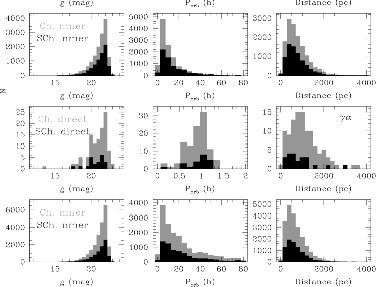
Figure 1: The distribution of $g$ magnitudes, orbital periods and distances for the four populations considered in this work (black for SCh. and gray for Ch. progenitors) when a cut off at $g=23$ mag is adopted for the WD components (see Table 1). The top and middle-top panels illustrate systems that evolved through $\alpha\alpha$ common envelopes, the bottom-middle and bottom panels systems that evolved through $\gamma\alpha$ common envelopes.

2 Synthetic binary population models

We create synthetic models for the Galactic population of double WDs by means of the binary population synthesis (BPS) method. We employ the code SeBa (Portegies Zwart & Verbunt, 1996; Toonen et al., 2012; Toonen & Nelemans, 2013) to simulate the formation and evolution of interacting binaries producing double WDs.

The initial binaries are generated according to a classical set-up for BPS calculations in the following way:

• We draw a mass from the initial mass function of Kroupa et al. (1993) within the range 0.1-100$\mathrm{M}_{\odot}$;

• The masses of the companion stars follow a uniform mass ratio distribution between 0 and 1 (Raghavan et al., 2010; Duchêne & Kraus, 2013; De Rosa et al., 2014; Cojocaru et al., 2017);

• The orbital separation $a$ is drawn from a uniform distribution in $\rm log(a)$ (Abt, 1983). Note that a log-normal distribution peaking at around $10^{5}$d is preferred observationally for Solar-type stars (Duquennoy & Mayor, 1991; Raghavan et al., 2010; Duchêne & Kraus, 2013; Moe & Di Stefano, 2017). This affects the number of simulated double WDs to less than 5% (Toonen et al., 2017);

• The eccentricities ($e$) follow a thermal distribution (Heggie, 1975): $f(e)=2e$ with $0<e<1$;

• We adopt a constant binary fraction of 50% which is appropriate for A-, F-, and G-type stars (Raghavan et al., 2010; Duchêne & Kraus, 2013; De Rosa et al., 2014; Moe & Di Stefano, 2017). A binary fraction of 75% (as observed for O- and B-type stars, e.g. Sana et al., 2012) would increase the numbers of double WDs by 36%;

• The orbital inclinations $i$ are obtained from a uniform distribution of $\sin i$.

It was shown in Toonen et al. (2014) that the main sources of differences between the synthetic models of different BPS codes is due to the choice of input physics and initial conditions. For double WDs, the most impactful assumption is that of the physics of unstable mass transfer; in which systems is the mass transfer not self-regulating, and what is the effect on the binary orbit and stellar components? Unstable mass transfer gives rise to a short phase in the evolution of a binary system in which both stars share a common-envelope (CE). Even though CE-evolution plays an essential role in the formation of compact binaries, and despite the enormous effort of the community, the CE-phase is poorly understood (e.g. Ivanova et al., 2013, for a review). For this reason we employ two different models for the CE-phase, model $\alpha\alpha$  and model $\gamma\alpha$, which are described below.

The classical model (model $\alpha\alpha$) is based on the energy budget (Paczynski, 1976; Tutukov & Yungelson, 1979; Webbink, 1984; Livio & Soker, 1988):

$$E_{\rm gr}=\alpha(E_{\rm orb,initial}-E_{\rm orb,final}),$$ (1)

where $E_{\rm gr}$ is the binding energy of the envelope mass, $E_{\rm orb}$ is the orbital energy, and $\alpha$ the efficiency with which orbital energy is consumed to unbind the CE. We approximate $E_{\rm gr}$ by:

$$E_{\rm gr}=\frac{GMM_{\rm env}}{\lambda R},$$ (2)

where $M$ is the mass of the donor star, $M_{\rm env}$ its envelope mass, $\lambda$ the envelope structure parameter, and $R$ the radius of the donor star. Here we adopt $\alpha\lambda=2$ as derived by Nelemans et al. (2000) by reconstructing the formation of the second WD for a sample of observed double WDs.

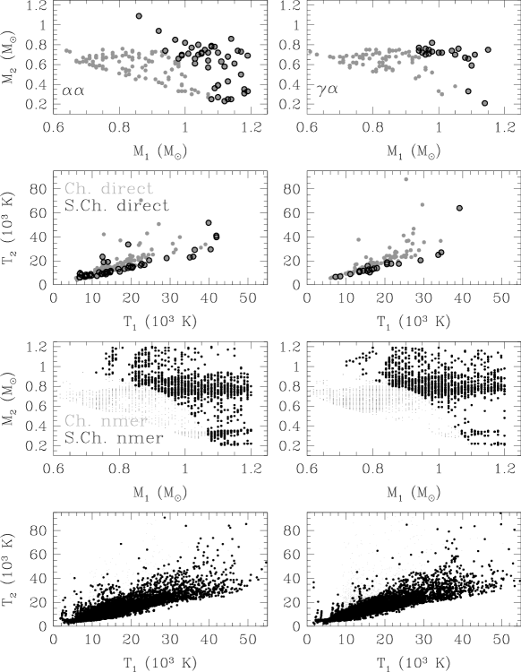
Figure 2: Comparison between the component masses and effective temperatures of the two WDs for the four populations considered in this work (see Table 1). The left panels illustrate systems that evolved through $\alpha\alpha$ common envelopes, the right panels systems that evolved through $\gamma\alpha$ common envelopes. Note that the SCh. progenitors (black circles) are a sub-population of the Ch. samples (gray circles).

The alternative model (model $\gamma\alpha$) is inspired by the (same) work of Nelemans et al. (2000). In order to explain the observed mass ratios of double WDs, Nelemans et al. (2000) propose an alternative CE-formalism, which is based on the angular momentum budget:

$$\frac{J_{\rm initial}-J_{\rm final}}{J_{\rm initial}}=\gamma\frac{\Delta M}{M+m},$$ (3)

where $J$ is the angular momentum of the binary, and $m$ the mass of the companion. We adopt $\gamma=1.75$ (see Nelemans et al., 2001). In model $\gamma\alpha$  when a CE develops, Eq. 3 is applied unless the binary contains a compact object or the CE is triggered by the Darwin-Riemann instability (Darwin, 1879; Hut, 1980). For double WDs, the first CE is typically simulated with the $\gamma$-parametrization, and the second with the $\alpha$-formalism.

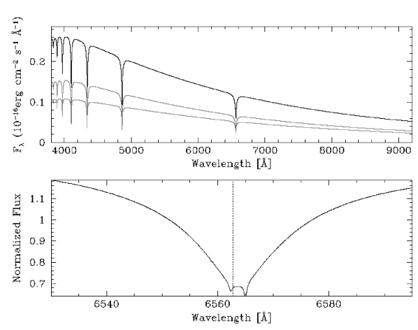
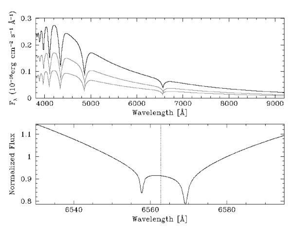
Figure 3: Top panels: two examples of simulated double WD spectra (black solid lines). The individual WD components are shown as gray solid lines. Bottom panels: a zoom-in to the H$\alpha$ line of the combined spectra. The temperatures and masses of the WD components are $M_{1}=0.76\,$M_⊙, $M_{2}=0.67\,$M_⊙, $T_{1}=8315$ K, $T_{2}=7715$ K (left panels) and $M_{1}=1.01\,$M_⊙, $M_{2}=0.72\,$M_⊙, $T_{1}=17980$ K, $T_{2}=13931$ K (right panels).

It has also been proposed that the first WD is not formed through a CE-phase, but through stable, non-conservative mass transfer (Woods et al., 2012; Passy et al., 2012; Ge et al., 2015). The effect on the orbit is a modest widening, similar to that of the $\gamma$-formalism. A BPS study of the implications on the double WD population of the increased stability of mass transfer, is beyond the scope of this paper.

To study the visibility of the double WDs in our Milky Way, we convolve the BPS data with the Galactic star formation history (SFH) and apply a WD cooling. The SFH is based on the model by Boissier & Prantzos (1999), which adopts a total mass in stars of 3.8$\times 10^{10}$ M_⊙ and is a function of both time and position in the Milky Way. Full details on our SFH model can be found in Toonen & Nelemans (2013), including information on the Galactic components adopted. The $ugriz$ magnitudes of the WDs are estimated by their distances, while taking into account extinction (Schlegel et al., 1998) and cooling through the evolutionary sequences. In this work we assume all the WDs to be composed of pure hydrogen-rich atmospheres, i.e. DA WDs, and hence adopt the cooling sequences developed for DA WDs of Holberg & Bergeron (2006); Kowalski & Saumon (2006); Tremblay et al. (2011). Knowing the magnitudes of each WD component we can easily derive the magnitudes of the double WD system by summing up the individual fluxes in each band. This is a valid assumption for close (unresolved) binaries such us the progenitors of SNIa. For more details of the Galactic model, see Toonen & Nelemans (2013). Here, we only consider systems where at least one component has a g-band magnitude below 23 magnitudes since observations of fainter systems would be extremely challenging. We also note that we only simulate the hydrogen-rich double WD population in the Galaxy, i.e. double DA WDs. We define the primary WD as the first formed WD, the secondary is the second formed WD. Hence, hereafter all parameters associated with the primary and secondary WDs will be denoted by the suffixes 1 and 2, respectively. It is also important to mention that, once the double-degenerate binaries are formed, we take into account angular momentum losses by gravitational wave radiation, which reduce the orbital separation until present time.

For the present work, and based on the above described numerical simulations, we define four populations of interest:

• The ’Ch. direct’ SNIa progenitor population, which comprises double WDs that merge within the Hubble time and with a total mass exceeding 1.3 $\mathrm{M}_{\odot}$  (we adopt this value as a lower limit since SNIa explosions occur near the Chandrasekhar mass).

• The ’SCh. direct’ progenitor population, which includes double WDs that merge within the Hubble time leading to sub-Chandrasekhar explosions. To select these systems we apply the condition $M_{2}>-10.2041\times(M_{1}-0.85)^{2}+0.805$ (or $M_{1}>-10.2041\times(M_{2}-0.85)^{2}+0.805$) provided by Shen et al. (2017), which selects massive primaries that have higher gravitational potentials and massive secondaries that yield more directly impacting accretion streams. These two processes make it more likely a sub-Chandrasekhar WD to explode.

• The ’Ch. nmer’ SNIa progenitor population, which is the same as population 1 (Ch. direct) but for WD binaries that do not merge within the Hubble time.

• The ’SCh. nmer’ population, which is the same as population 2 (SCh. direct) but for systems that do not merge within the Hubble time.

As we will show in Section 5, considering the non-merger samples (i.e. the Ch. nmer and SCh. nmer populations) allows deriving more sound results regarding the observational properties of SNIa progenitors. In Table 1 we provide the number of double WDs in each population depending on the common envelope prescription used in our simulations.

The $g$ magnitude, orbital period and distance distributions as well as the comparison between the component masses and effective temperatures of the two WDs for the four considered populations are illustrated in Figure 1 and Figure 2. From the Figures one can clearly see that the number of non-merger SNIa progenitors is significantly larger than that of direct progenitors, and that the orbital period distributions for direct and non-merger systems are substantially different.

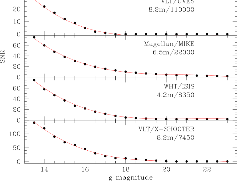
Figure 4: SNR as a function of $g$ magnitude (assuming 0.5 magnitude bins) for the telescope/instrument pairs considered in this work, and fixing the exposure time at 10 minutes (black solid dots). The red solid lines are third order polynomial fits to the data. The telescope apertures and resolving powers of the spectrographs are also indicated.

3 The double-degenerate synthetic spectra

The population synthesis code described in the previous section has provided us with masses, effective temperatures, surface gravities and radii of the binary components, as well as with orbital periods, orbital inclinations and distances to each SNIa progenitor in four different populations. Here we develop a method for obtaining their synthetic spectra.

In a first step we obtain a synthetic spectrum for each WD component by interpolating the corresponding effective temperature and surface gravity values on an updated grid of model atmosphere spectra of Koester (2010). The grid contains 612 spectra of effective temperatures ranging from 6,000 K to 10,000 K in steps of 250 K, from 10,000 K to 30,000 K in steps of 1,000 K, from 30,000 K to 70,000 K in steps of 5,000 K and from 70,000 K to 100,000 K in steps of 10,000 K, and surface gravities ranging between 6.5 and 9.5 dex in steps of 0.25 dex for each effective temperature. The model spectra provide the astrophysical fluxes at the surface of the WDs ($F_{\mathrm{wd}}$), which we convert into observed fluxes ($f_{\mathrm{wd}}$) using the flux scaling factors. That is, for each white dwarf

$$\frac{f_{\mathrm{wd}}}{F_{\mathrm{wd}}\times\pi}=\left(\frac{R_{\mathrm{wd}}}{d}\right)^{2}$$ (4)

where $R_{\mathrm{wd}}$ is the white dwarf radius and $d$ is the distance, parameters that are both known for each SNIa progenitor. The model spectra are provided in vacuum wavelengths, which we convert into air wavelengths.

The orbital periods of the SNIa progenitors in our four populations are short ($\la$80 hours, especially those that merge within the Hubble time, $\la$1.5 hours; see Figure 1). Hence, we need to apply a wavelength shift due to the corresponding radial velocity variation (shortened by the inclination factor) to each WD synthetic spectrum component. Moreover, the spectrum of each WD is affected by the corresponding gravitational redshift.

We use the following equations to get the gravitational redshift $Z$ for each WD (in km/s)

$$Z_{1}=0.635\left(\frac{M_{1}}{R_{1}}+\frac{M_{2}}{a}\right),\hskip 14.22636ptZ_{2}=0.635\left(\frac{M_{2}}{R_{2}}+\frac{M_{1}}{a}\right);$$ (5)

where the masses ($M_{1}$, $M_{2}$) and radii ($R_{1}$, $R_{1}$) are in solar units and $a$ is the orbital separation, also known for each binary from Kepler’s third law and given in solar radii. This expression takes into account the gravitational potential acting on a WD owing to its WD companion. We convert the gravitational redshifts into wavelength shifts that we then apply to each WD synthetic spectrum.

The maximum radial velocity shift $K_{1}$ for WD₁ is obtained following

$$K_{\mathrm{1}}=\left[\frac{2\pi G\,(M_{2}\sin i)^{3}}{\mbox{$P_{\mathrm{orb}}$}\,(M_{1}+M_{2})^{2}}\right]^{1/3}$$ (6)

with $i$ the orbital inclination, $P_{\mathrm{orb}}$  the orbital period and $G$ the gravitational constant. We then obtain the maximum radial velocity shift $K_{2}$ for WD₂ as $K_{1}\frac{M_{1}}{M_{2}}$. The maximum radial velocity shifts are converted into wavelength shifts and applied to the WD synthetic spectra. We assume a zero systemic velocity in all cases.

We finally obtain the double-degenerate (combined) spectrum by adding the observed fluxes of each WD component, corrected both by the gravitational and maximum radial velocity shifts. Two examples are shown in Figure 3, where we also display a zoom-in to the spectra around the H$\alpha$ line region. The H$\alpha$ line is typically used for identifying double-lined binaries (e.g. Koester et al., 2001). Double-lined binaries allow sampling the orbital motion of the two stars, hence one can derive the radial velocity semi-amplitudes and the mass ratio, which together with some elaborated further analysis allows deriving the component masses of the WDs (see for example Maxted et al. 2002; Rebassa-Mansergas et al. 2017). With the component masses and the orbital periods at hand one can then easily evaluate whether or not the binary will merge within the Hubble time and explode as a SNIa and/or a sub-Chandrasekhar SNIa, or simply form a massive WD.

Figure 3 shows two WD synthetic spectra from our Ch. direct population. Both display double-lined profiles from which we would be able to measure the orbital periods and component WD masses and hence identify such system as a SNIa progenitors.

Figure 5: A zoom-in to the H$\alpha$ region of the synthetic spectra of four Ch. direct SNIa progenitors (i.e. double WDs that merge within the Hubble time and with a total mass exceeding 1.3 $\mathrm{M}_{\odot}$) as observed by the five different telescope/spectrograph configurations considered in this work. For comparison, we also show the “ideal” spectra, i.e. spectra not affect by any observational bias, of the four binaries. The temperatures and masses of the WD components are $M_{1}=0.83\,$M_⊙, $M_{2}=0.68\,$M_⊙, $T_{1}=15778$ K, $T_{2}=15472$ K (top left panels); $M_{1}=1.13\,$M_⊙, $M_{2}=0.68\,$M_⊙, $T_{1}=35076$ K, $T_{2}=22896$ K (top right panels); $M_{1}=1.10\,$M_⊙, $M_{2}=0.39\,$M_⊙, $T_{1}=19234$ K, $T_{2}=33677$ K (bottom left panels) and $M_{1}=0.81\,$M_⊙, $M_{2}=0.76\,$M_⊙, $T_{1}=15107$ K, $T_{2}=14533$ K (bottom right panels)

4 Observational effects

The double WD synthetic spectra obtained in the previous section represent ideal spectra in the sense that they are given at virtually infinity signal to noise ratio (SNR) as well as at a resolution which is typically larger than the ones provided by current spectrographs. Therefore, in order to evaluate whether the double WDs would be clearly detected as double-lined binaries, we require incorporating observational effects in the synthetic spectra, i.e. adding artificial noise and downgrading the spectral resolution. To that end we evaluate how the synthetic spectra of our four selected SNIa progenitor populations would look like if these objects were observed by the following telescopes/spectrographs: the 8.2m Very Large Telescope (VLT) equipped with the UVES spectrograph ($R=$110,000), the VLT equipped with X-Shooter ($R=7,450$), the 4.2m William Herschel Telescope (WHT) equipped with ISIS ($R=8,350$), the 6.5m Magellan Clay telescope equipped with the MIKE spectrograph ($R=22,000$) and the 10.4m Gran Telescopio Canarias (GTC) equipped with OSIRIS ($R=2500$). The choice of these telescopes/spectrographs was made with the aim of covering a wide range of telescope apertures (which translate into different SNR for the same spectrum assuming the same exposure time) as well as spectral resolutions.

It becomes clear from Figure 1 that the orbital periods of the direct SNIa progenitors (both the Ch. direct and SCh. direct populations) are very short ($\la 1.5$ hours), independently of the common envelope formalism adopted. This implies the exposure times need to be short if we were to observe such systems, otherwise we would not sample enough points of the radial velocity curves and, more importantly, we would not be able to distinguish the double lines due to orbital smearing. We thus assume an exposure time of 10 minutes, which is a good comprise to avoid orbital smearing and to have enough radial velocities sampling the orbital phases.

Thus fixing a 10 minute exposure time, we determined the expected SNR as a function of $g$ magnitude for each of our selected telescopes/instruments. We did this by making use of the available exposure time calculators for each telescope/instrument pair. In all cases we assumed a moon phase of 0.5 (or gray time), an airmass of 1.5 and a seeing of 1”. We fitted third order polynomials to the obtained SNR versus magnitude relations, which we illustrate in Figure 4 (red solid lines). From these equations we estimated the SNR of all synthetic spectra. From these values, and assuming a Gaussian noise distribution, we were able to add artificial noise to the synthetic spectra. Before that, the spectra were downgraded to the required spectral resolving power.

Table 2: Number of systems that would be identified as SNIa progenitors for the four populations considered in this work. We provide the numbers for each combination of telescope/spectrograph and CE envelope formalism adopted.

Population	CE formalism	GTC/OSIRIS	Mag./MIKE	VLT/UVES	WHT/ISIS	VLT/X-Shooter
Ch. direct	$\alpha\alpha$	3	5	1	1	2
	$\gamma\alpha$	0	3	0	1	1
SCh. direct	$\alpha\alpha$	3	2	0	0	1
	$\gamma\alpha$	0	0	0	0	0
Ch. nmer	$\alpha\alpha$	16	77	7	22	47
	$\gamma\alpha$	15	79	6	15	48
SCh. nmer	$\alpha\alpha$	6	25	2	8	19
	$\gamma\alpha$	3	24	2	6	17

As it can be clearly seen from Figure 4, only bright objects ($g<17$ mag) would achieve a SNR larger than 10 if observed by the combinations of telescope aperture and spectral resolutions considered, except for the VLT/UVES pair, where only the brightest targets ($g\leq 15$ mag) would pass this cut. This implies the majority of both Ch. and SCh. SNIa direct progenitors would be associated to rather low SNR spectra (since most objects have magnitudes above $g=18$ mag, see Figure 1), which is expected to affect considerably the detection of the double-lined profiles in the spectra. This situation changes for the Ch. nmer and the SCh. nmer populations, that we recall include those SNIa progenitors that do not merge within the Hubble time. In these cases the orbital periods are considerably longer (between 10–80 hours; Figure 1), thus allowing increasing the exposures times to more than 10 minutes since we would not be affected by orbital smearing. However, since at the time of a hypothetical observing run one would not have at hand any previous information regarding the orbital periods, we decided to keep the exposure times fixed at 10 minutes for the non-merger populations too.

In Figure 5 we show the synthetic spectra zoomed to the H$\alpha$ region for the five telescope/instrument pairs considered of four direct SNIa progenitors. As we have already mentioned, H$\alpha$ is a widely common spectral feature used to both identify double-lined binaries and to measure the orbital periods and component masses (Koester et al., 2001; Maxted et al., 2002; Rebassa-Mansergas et al., 2017). Inspection of Figure 5 reveals a wide variety of different possibilities for the clear identification of the double-lined profiles. For instance, these can be easily identified in the spectra illustrated in the top left panels in all cases except when considering the GTC/OSIRIS configuration, where the low resolution is not enough to clearly resolve the two absorption lines despite the high SNR achieved. Conversely, only when considering the GTC/OSIRIS pair we can clearly identify the profiles when inspecting the spectra illustrated in the top-right panels. In the bottom-left panels, the spectra resulting from the Magellan/MIKE, VLT/XShooter and GTC/OSIRIS configurations reveal the two absorption profiles for this particular WD binary, whilst no double absorption profiles can be detected in any of the spectra displayed in the bottom-right panels. This implies we would not be able to measure the WD masses for this system and, consequently, we would not detect it as a SNIa progenitor.

In the next Section we analyse in detail how the observational effects here described affect the detectability of the SNIa progenitor population as a whole.

5 Results

In order to evaluate the impact of the observational effects described in the previous section in the detection of double-lined profile WD binaries we provide in Table 2 the number of WD binaries that would be able to be identified as SNIa progenitors (based on the clear identification of the two profiles in the H$\alpha$ region) for the four populations considered in this work, taking into account both the CE formalism adopted and the different telescope/spectrograph configurations. Table 2 reveals that the number of identified progenitors does not depend much on the CE formalism, being the only difference the fact that, generally, a slightly less number of systems is identified from the populations evolving through $\gamma\alpha$ CEs. It also becomes clear that the number of identified progenitors varies considerably depending on the telescope/spectrograph configuration, as expected from Figure 5.

Independently of the CE formalism and telescope/spectrograph configuration, Table 2 also shows that the number of identified SNIa progenitors is very low as compared to the total number of progenitor systems in the populations (Table 1). If we consider the Magellan/MIKE pair and the $\alpha\alpha$ synthetic populations, which results in the maximum number of SNIa progenitors identified, then the fractions of SNIa progenitors that are expected to be identified are 3% for the Ch. direct population, 4% for the SCh. direct population, 0.5% for the Ch. nmer population and 0.3% for the SCh. nmer population. Taking into account that the complete $\alpha\alpha$ WD binary synthetic population contains $\sim$370,000 objects, of which $\sim$237,000 are unresolved, then the estimated probabilities for finding SNIa progenitors are ($2.1\pm 1.0)\times 10^{-5}$ (Ch. direct population), $(0.8\pm 0.4)\times 10^{-5}$ (SCh. direct population) $(3.2\pm 0.4)\times 10^{-4}$ (Ch. nmer population) and $(1.1\pm 0.2)\times 10^{-4}$ (SCh. nmer population). The uncertainties in the probabilities are obtained assuming Poisson errors in the values provided in Table 2. We obtain similar values when considering the $\gamma\alpha$ synthetic populations. The probabilities are lower for the SCh. populations since these objects are a sub-sample of the Ch. populations (see Figure 2). Indeed, all the identified SNIa progenitors in the SCh. populations are also included in the Ch. direct populations.

Judging from Table 2, the most efficient telescope aperture/resolution combination seems to be the one provided by the Magellan/MIKE pair, followed by the VLT/X-Shooter. In both cases, the apertures are large enough for achieving higher SNR spectra and the resolving powers are high enough for sampling the double-lined profiles. This is also true for the WHT/ISIS configuration, which results in a similar resolving power as the one by the VLT/X-Shooter, but for a lower number of systems due to the smaller telescope aperture. The GTC/OSIRIS pair achieves the highest SNR, however the spectral resolution is rather low in this case, thus making it difficult to sample the two absorption profiles and hence reducing considerably the number of identified progenitors. The VLT/UVES pair is the less efficient configuration for identifying SNIa progenitors. This is due to the extremely high resolving power achieved, which limits considerably the SNR of the obtained spectra. All this can clearly be seen in the left panels of Figure 6, where we illustrate the orbital inclination of the binaries that clearly show double lines in their spectra as a function of their $g$ magnitudes for the five telescope aperture/spectrograph configurations considered. Since the number of potential progenitors that are able to be identified does not dramatically depend on the CE formalism used (Table 2), we choose for this exercise the $\gamma\alpha$ samples, since the ensemble properties of the binaries resulting from these simulations better agree with those derived from observations (Nelemans et al., 2000; Toonen et al., 2012).

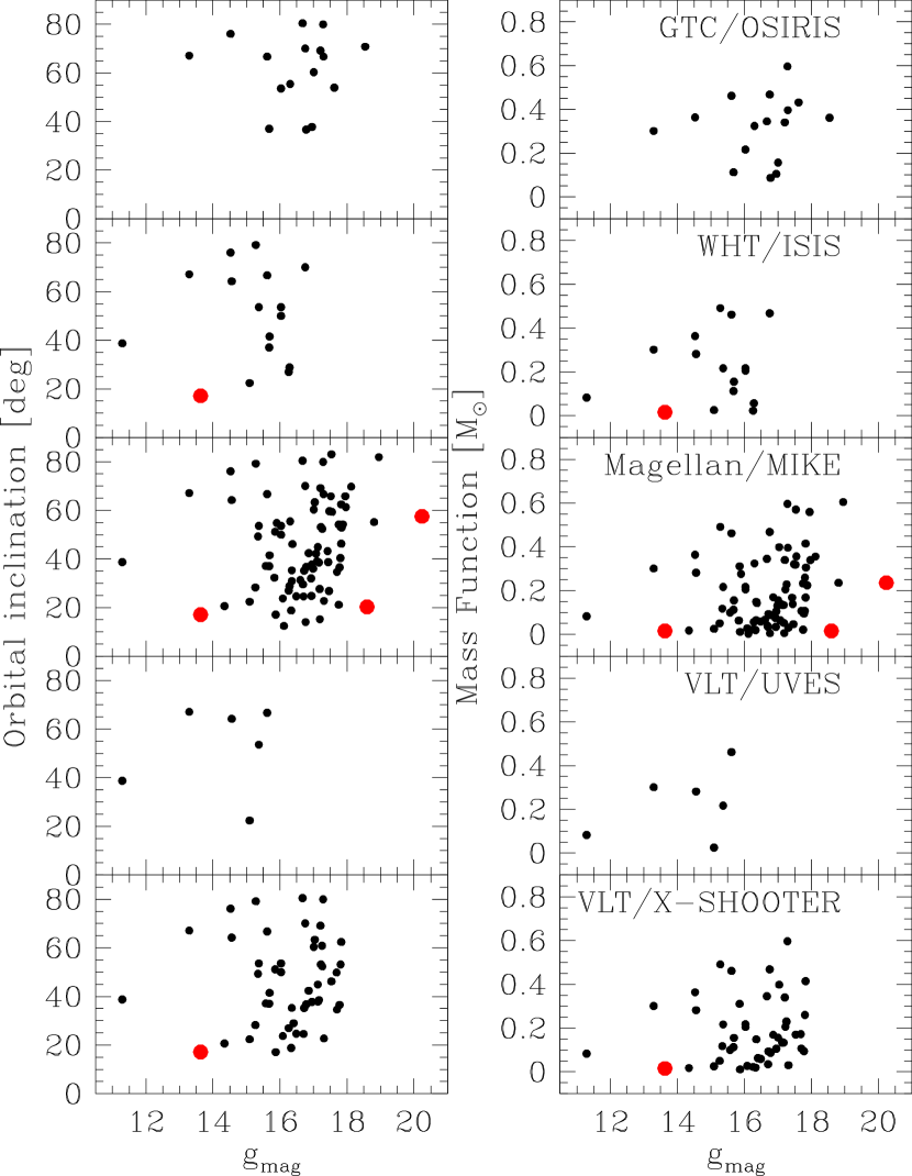
Figure 6: Left panels: orbital inclination as a function of $g$ magnitude for all the SNIa progenitors for which the simulated spectra clearly display double-lined profiles. Large red solid dots indicate direct SNIa progenitors, black solid dots non-merger progenitors within the Hubble time. Right panels: mass function as a function of $g$ magnitude for the same systems. The corresponding telescope/spectrograph pairs are indicated in the top right of each panel.

From Figure 6 (left panels) it becomes obvious that, as expected, larger aperture telescopes are more suitable for identifying the double-lined profiles in the spectra of fainter objects, being $\sim$19 mag the magnitude limit. This is the case for the GTC/OSIRIS, Magellan/MIKE and VLT/X-Shooter configurations. However, it is also clear that, as we mentioned before, not only the telescope aperture but also the resolving power of the instrument affects the magnitude limit for identifying the double lines in the spectra. For example, in the case of the VLT equipped with the UVES instrument, the double lines can only be identified for systems with $g$ magnitudes below 16 mag due to the extremely high resolving power achieved (which limits the SNR). The relatively high resolving power of the MIKE instrument, followed by the X-Shooter spectrograph, makes this the ideal instrument among the larger aperture telescopes for the detection of the double lines.

The orbital inclination plays also an important role for the detectability of the double lines. As can be seen in the left panels of Figure 6, it is not possible to identify double-lined systems when the inclinations are lower than $\sim$20 degrees, simply because the two lines are smeared. This effect is stronger when considering the GTC equipped with the low resolution OSIRIS instrument. In this case, the orbital inclinations need to be higher than $\sim$40 degrees.

In the right panels of Figure 6 we display the mass function versus the $g$ magnitudes for the same systems displayed in the left panels. The mass function is defined as:

$$m=\frac{K_{\mathrm{1}}^{3}P_{\mathrm{orb}}}{2\pi G}=\frac{(M_{2}\sin i)^{3}}{(M_{1}+M_{2})^{2}},$$ (7)

where $M_{1}$ is in this case the brighter star in a binary and $K_{1}$ its semi-amplitude velocity. Since the mass function depends only on $P_{\mathrm{orb}}$ and $K_{\mathrm{1}}$, values that can be relatively easy determined observationally even for single-lined binaries, this quantity may help in providing clues on how to efficiently target SNIa progenitors. However, as it can be seen in the right panels of Figure 6, there seems to be no obvious trend, since a wide range of values are possible among all possible SNIa progenitors.

We conclude identifying both direct and non-merger and both Ch. and SCh. SNIa progenitors with our current optical telescopes and instrumentation is extremely challenging due to their intrinsic faintness.

6 Discussion

The results presented in this paper demonstrate that identifying double-degenerate SNIa progenitors is extremely hard due to observational biases. In other words, the probability for detecting a double WD SNIa progenitor in the Galaxy based on the detection of double-lined absorption profiles in the spectrum is very low with our current instrumentation, since the vast majority of these systems are intrinsically faint. Increasing the current size of known WDs e.g. by analysing the recent superb sample of $\sim$8500 Gaia data release 2 WDs within 100pc from the Sun (Jiménez-Esteban et al., 2018), does not seem to be the solution given that possible SNIa progenitors within this sample are also expected to be faint. In the following we analyse possible ways for increasing the probability of detection and discuss alternative ways for finding SNIa double WD progenitors.

6.1 The next generation of large-aperture telescopes

A clear way to move forward includes improving our observational facilities. Fortunately, the next generation of large-aperture ($\simeq 30$m) optical telescopes such as the European Extremely Large Telescope (E-ELT; McPherson et al., 2012), the Great Magellan Telescope (GMT; Sheehan et al., 2012) or the Thirty Meter Telescope (TMT; Skidmore et al., 2015) will allow observing down to deeper magnitudes at a much lower cost in terms of exposure times. This is expected to increase the probability of detecting double WD SNIa progenitors. For instance, if we assume these telescopes to achieve a reasonably high SNR for a 10 minute exposure for objects down to 23 magnitudes (i.e. we are not limited by the noise in the spectrum but on the orbital inclination of the systems for detecting the double-lined profiles), then the probability for finding e.g. Ch. direct SNIa progenitors increases one order of magnitude from $(2.1\pm 1.0)\times 10^{-5}$ to $(3.9\pm 0.4)\times 10^{-4}$.

6.2 Uncertainties in our numerical simulations

It is possible that our numerical simulations predict a low number of SNIa progenitors, in which case we would be underestimating the probability of their detection. The observed SNIa rate integrated over a Hubble time is $(13\pm 1)\times 10^{-4}$M${}_{\odot}^{-1}$ (Maoz & Graur, 2017, and references therein). On the other hand the integrated rates in our simulations for Chandrasekhar mergers of double white dwarfs are a factor of a few lower than the observed rate ($(4.2-5.5)\times 10^{-4}$M${}_{\odot}^{-1}$), which, however, does not significantly affect the detection probabilities.

It is important to emphasize that the evolution of double WD binaries is not well understood yet and that our adopted modeling of CE evolution (both the $\alpha$ and $\gamma$ formalisms) may not be adequate (Woods et al., 2012; Passy et al., 2012; Ge et al., 2015). A better treatment of mass transfer could help in increasing the number of SNIa progenitors. Hence, exploring population synthesis models including a phase of stable non-conservative mass transfer (unfortunately, not yet implemented in any BPS code) rather than a first CE phase seems them to be a worthwhile exercise. An additional factor to take into account is that our results are based on the outcome of two synthetic double WD binary populations that differ only with respect to the CE phase. Uncertainties on other physical processes, such as the stability or mass accretion efficiency of mass transfer, affect the double white dwarf population as well, but to a lesser degree.

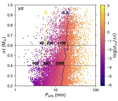
Figure 7: Relative error on the chirp mass $\sigma_{{\cal M}}/{\cal M}$ in period-chirp mass parameter space. The dashed vertical lines are iso-relative-error contours for $\log$($\sigma_{{\cal M}}/{\cal M}$) $=$ -3 (yellow), -2 (pink) and -0.5 (blue), equivalent to $\sigma_{{\cal M}}/{\cal M}=0.1\%$ (yellow), $1\%$ (pink) and $\sim 32\%$ (blue). The values on top of the horizontal lines indicate the number of systems with a given relative error limit (i.e. systems to the left of the dashed vertical lines) and with a chirp mass higher than 0.4 or 0.6 M_⊙ (systems above the horizontal lines).

We also need to bear in mind that our synthetic double WD space density may be underestimated. Recently, our synthetic space density values were verified by Toonen et al. (2017) with a comparison between common synthetic WD systems based on the same BPS set-up employed here and the nearly-complete volume-limited sample of WDs within 20 pc. The space density of single WDs and resolved WD plus main sequence binaries (which represent the most common WD systems) are correctly reproduced within a factor 2. The synthetic models of double WDs are in good agreement with their observed number in 20pc, albeit given their current small number statistics in this sample (1 + 4 candidates). Another constraint on the space density of double WDs can be made by studying the ratio $f$ of double WDs to single WDs. From the above-mentioned 20pc sample, $f=0.008-0.04$ for (unresolved) double WDs, whereas our model $\alpha\alpha$ gives $f\approx 0.02$, and model $\gamma\alpha$ $f\approx 0.04$ (see Toonen et al., 2017). Based on radial velocity measurements of a sample of 46 DA WDs Maxted & Marsh (1999) deduce $f=0.017-0.19$ with a 95% probability for periods of hours to days. From a statistical approach of the maximum radial velocity measurement of $\sim$4000 WDs in SDSS, Badenes & Maoz (2012) deduce $f=0.03-0.20$ for orbits smaller than 0.05AU. With a similar approach on 439 WDs from the SPY survey, Maoz & Hallakoun (2017) find $f=0.103$ with a random error of $\pm 0.02$ and a systematic error of $\pm 0.015$ for orbits within 4AU. From a joint likelihood analysis of these two samples, $f=0.095\pm 0.020$ (random)$\pm 0.010$ (systematic) (Maoz et al., 2018). These measurements may imply that our synthetic double WD space densities are underestimating the true space density, but not by a factor more than 2-5, which does not significantly change our calculated value of the probability of finding double WD SNIa progenitors.

6.3 Eclipsing double WDs

It is important to emphasise that we have considered the detection of SNIa progenitors based only on the clear identification of double-lined profiles, which allows measuring the WD component masses. An additional way of measuring the masses involves analysing the light curves of eclipsing systems (e.g. Parsons et al., 2011). Since the orbital inclinations and mass ratios can be relatively well constrained in these cases, by measuring the orbital periods and deriving the masses of the brightest components (e.g. by fitting the observed spectrum with model atmosphere spectra), one can then derive precise values of the masses of the two WDs. However, deriving the semi-amplitude velocity of at least one of the WD components is required for accurately determining the WD masses. Thus, so far only 7 eclipsing double WD binaries are known for which the WD masses have been accurately determined, none of them being direct SNIa progenitors: SDSS J0651+2844 (Hermes et al., 2012), GALEX J1717+6757 (Hermes et al., 2014), NLTT 11748 (Kaplan et al., 2014), SDSS J0751-0141 (Kilic et al., 2014), CSS 41177 (Bours et al., 2015), SDSS J1152+0248 (Hallakoun et al., 2016) and SDSS J0822+3048 (Brown et al., 2017). It is important to keep in mind however that the identification of a large number of eclipsing WD binaries is expected from the forthcoming Large Synoptic Survey Telescope (LSST; Tyson, 2002). Korol et al. (2017) predicted the number of eclipsing WD binaries LSST will identify is close to one thousand. It has to be emphasised that the authors of that paper employed the same numerical simulation code than us, which easily allows us to obtain synthetic spectra for their eclipsing systems and to thus evaluate how many of them are potential SNIa progenitors and for how many we could derive the semi-amplitude velocities of at least one WD component with our adopted telescopes/spectrographs. From the $\sim$1000 eclipsing double WDs that LSST is expected to identify, only 3–7 are found to be direct Ch. SNIa progenitors depending on the CE formalism used (note that no SCh. progenitors are in the samples) and unfortunately none of them would be suitable for radial velocity follow-up observations due to their intrinsic faintness.

6.4 Gravitational waves and LISA

An alternative way of detecting SNIa progenitors is by exploiting their gravitational wave (GW) radiation. Double WD binaries with orbital periods from a few minutes to one hour are expected to be detected through GW radiation by the Laser Interferometer Space Antenna (LISA; Amaro-Seoane et al., 2017). Using the same population synthesis code and model assumptions as in this paper, Korol et al. (2018) showed that LISA is expected to individually resolve $>10^{5}$ double WD binaries across the Milky Way. Here we investigate how many of the LISA detections are expected to be SNIa progenitors.

Long timescales on which double WDs evolve (typically $\sim$Myr) imply that LISA will catch them in the inspiral phase. During inspiral the evolution of the GW signal depends on the so-called chirp mass, a particular combination of the individual WD masses, defined as ${\cal M}=(M_{1}M_{2})^{3/5}(M_{1}+M_{2})^{-1/5}$. This means that individual masses $M_{1}$ and $M_{2}$ are difficult to estimate from GW data and, typically, this requires additional assumptions. Thus, in this work we use the chirp mass to select SNIa progenitors among LISA detections. In particular, we adopt two thresholds: $0.6\,$M_⊙ and $0.4\,$M_⊙. The first one comes from considering a binary with equal mass components and the total mass $M=1.38\,$M_⊙. The last one is determined from our catalogues as the minimum chirp mass among the binaries with $M>1.38\,$M_⊙. To compute the GW signal for binaries in the two mock catalogues we employ the Mock LISA Data Challenge (MLDC) pipeline, designed for the analysis of Galactic GW sources (for details see Littenberg, 2011). We model double WD waveforms using a set of 9 parameters: GW amplitude $\cal{A}$, GW frequency $f=2/P_{\rm orb}$, the frequency evolution or chirp $\dot{f}$, orbital inclination $i$, polarization angle $\psi$, initial GW phase $\phi_{0}$ and binary coordinates on the sky. We estimate the respective uncertainties by computing Fisher Information Matrix (FIM, e.g. Shah et al., 2012). We adopt the most recent LISA mission design and the noise model from Amaro-Seoane et al. (2017), i.e. a three-arm configuration with $2.5\times 10^{6}\,$km arm length. Finally, we assume the duration of the mission to be of 4 yr.

From GW data the chirp mass can be determined by taking the lowest order in a post-Newtonian expansion of the waveform’s phase, i.e.

$${\cal M}=\frac{c^{3}}{G}\left(\frac{5}{96}\pi^{-8/3}{\dot{f}}\right)^{3/5}f^{11/5},$$ (8)

where $f$ and $\dot{f}$ are direct GW observables, which uncertainties and correlation coefficient can be extracted from the FIM. We find 1400 (1100) double WDs with ${\cal M}>0.6\,$M_⊙ and a relative error on the chirp mass $<30\%$ for our $\alpha\alpha$ ($\gamma\alpha$) catalogues. Using the threshold of $0.4\,$M_⊙ we find 4000 (3300) binaries. In Fig. 7 we represent the relative error on the chirp mass $\sigma_{{\cal M}}/{\cal M}$ for double WDs detected by LISA in the period - chirp mass parameter space. Figure 7 shows a gradual decrease in $\sigma_{{\cal M}}/{\cal M}$ from longer to shorter orbital periods. This is because short period sources have larger chirps, which makes it easier to determine the chirp mass and its uncertainty. Furthermore, binaries with large chirp masses have large GW amplitudes (${\cal A}\propto{\cal M}^{5/3}$), that facilitate their detection. These two facts reflects in high number of SNIa progenitors detected by LISA.

7 Summary and conclusions

With the aim of evaluating the observability of double-degenerate SNIa progenitors we simulated the double WD binary population in the Galaxy and obtained synthetic optical spectra for each progenitor. To that end we considered a set of ground-based telescopes of different diameter sizes and equipped with spectrographs covering a wide range of spectral resolutions.

We analysed the detectability of clear H$\alpha$ double-lined profiles in the synthetic spectra and considered a positive detection as a sufficient condition for deriving accurate orbital periods and component masses of the two WDs. In these cases we assumed the systems would be identified as SNIa progenitors. Due to the intrinsic faintness of the double-degenerate SNIa population, our simulations indicate that only a handful of objects are expected to be found with clear double-lined profiles in their spectra, which resulted in a probability of finding double WD SNIa progenitors of $(2.1\pm 1.0)\times 10^{-5}$ (for the direct classical Chandrasekhar progenitor population) and $(0.8\pm 0.4)\times 10^{-5}$ (for the direct sub-Chandrasekhar progenitor population). These results do not depend significantly on the formalism of common envelope adopted. We found the best combination of telescope/spectrograph for finding SNIa progenitors is the Magellan Clay/MIKE, followed by the VLT/X-Shooter.

Forthcoming large-aperture telescopes are expected to increase the probability for finding double WD SNIa progenitors by $\sim$1 order of magnitude. Although this is a considerably large increase, the probability for finding these objects remains low ($\sim 10^{-4}$). We also analysed how eclipsing binaries can help in increasing the number of identified SNIa progenitors, and concluded that, even with the outcome of LSST, the probability remains unchanged. Our results thus clearly show that identifying double-degenerate progenitors of SNIa is extremely challenging. It is not surprising then that current observational studies have failed at finding such systems. We hence conclude that the lack of observed double WD SNIa progenitors is not a sufficient condition for disregarding the double-degenerate channel nor the sub-Chandrasekhar models for SNIa.

Fortunately, thanks to the new window of gravitational wave radiation observations that LISA will open, the expectations for finding double WD SNIa progenitors are highly encouraging. Our results show that LISA should be able to find $\ga$1000 SNIa progenitors by means of measuring the chirp masses of the WD binaries, which will allow us to robustly confirm or disprove (in the case of no detections) the relevance of double WD binaries for producing SNIa. It has to be noted however that follow-up spectroscopic/photometric observations will be required to measure the individual masses of the identified progenitors.

References

- Abt (1983) Abt H. A., 1983, Annual Review of Astronomy and Astrophysics, 21, 343
- Amaro-Seoane et al. (2017) Amaro-Seoane P., et al., 2017, preprint, (arXiv:1702.00786)
- Astier & Pain (2012) Astier P., Pain R., 2012, Comptes Rendus Physique, 13, 521
- Aznar-Siguán et al. (2013) Aznar-Siguán G., García-Berro E., Lorén-Aguilar P., José J., Isern J., 2013, MNRAS, 434, 2539
- Badenes & Maoz (2012) Badenes C., Maoz D., 2012, ApJ, 749, L11
- Benz et al. (1989) Benz W., Thielemann F.-K., Hills J. G., 1989, ApJ, 342, 986
- Boissier & Prantzos (1999) Boissier S., Prantzos N., 1999, MNRAS, 307, 857
- Bours et al. (2015) Bours M. C. P., Marsh T. R., Gänsicke B. T., Parsons S. G., 2015, MNRAS, 448, 601
- Breedt et al. (2017) Breedt E., et al., 2017, MNRAS, 468, 2910
- Brown et al. (2013) Brown W. R., Kilic M., Allende Prieto C., Gianninas A., Kenyon S. J., 2013, ApJ, 769, 66
- Brown et al. (2016) Brown W. R., Kilic M., Kenyon S. J., Gianninas A., 2016, ApJ, 824, 46
- Brown et al. (2017) Brown W. R., Kilic M., Kosakowski A., Gianninas A., 2017, ApJ, 847, 10
- Cojocaru et al. (2017) Cojocaru R., Rebassa-Mansergas A., Torres S., García-Berro E., 2017, MNRAS, 470, 1442
- Darwin (1879) Darwin G., 1879, Phil. Trans. Roy. Soc., 170, 447
- De Rosa et al. (2014) De Rosa R. J., et al., 2014, MNRAS, 437, 1216
- Duchêne & Kraus (2013) Duchêne G., Kraus A., 2013, ARA&A, 51, 269
- Duquennoy & Mayor (1991) Duquennoy A., Mayor M., 1991, A&A, 248, 485
- García-Berro et al. (2016) García-Berro E., Soker N., Althaus L. G., Ribas I., Morales J. C., 2016, New Astron., 45, 7
- Ge et al. (2015) Ge H., Webbink R. F., Chen X., Han Z., 2015, ApJ, 812, 40
- Geier et al. (2010) Geier S., Heber U., Kupfer T., Napiwotzki R., 2010, A&A, 515, A37
- González Hernández et al. (2012) González Hernández J. I., Ruiz-Lapuente P., Tabernero H. M., Montes D., Canal R., Méndez J., Bedin L. R., 2012, Nature, 489, 533
- Guillochon et al. (2010) Guillochon J., Dan M., Ramirez-Ruiz E., Rosswog S., 2010, ApJ, 709, L64
- Hallakoun et al. (2016) Hallakoun N., et al., 2016, MNRAS, 458, 845
- Han & Podsiadlowski (2004) Han Z., Podsiadlowski P., 2004, MNRAS, 350, 1301
- Heggie (1975) Heggie D. C., 1975, MNRAS, 173, 729
- Hermes et al. (2012) Hermes J. J., et al., 2012, ApJ, 757, L21
- Hermes et al. (2014) Hermes J. J., et al., 2014, MNRAS, 444, 1674
- Hillebrandt et al. (2013) Hillebrandt W., Kromer M., Röpke F. K., Ruiter A. J., 2013, Frontiers of Physics, 8, 116
- Holberg & Bergeron (2006) Holberg J. B., Bergeron P., 2006, AJ, 132, 1221
- Howell (2011) Howell D. A., 2011, Nature Communications, 2, 350
- Hut (1980) Hut P., 1980, A&A, 92, 167
- Iben & Tutukov (1984) Iben Jr. I., Tutukov A. V., 1984, ApJS, 54, 335
- Ivanova et al. (2013) Ivanova N., et al., 2013, A&ARv, 21, 59
- Jiménez-Esteban et al. (2018) Jiménez-Esteban F. M., Torres S., Rebassa-Mansergas A., Skorobogatov G., Solano E., Cantero C., Rodrigo C., 2018, preprint, (arXiv:1807.02559)
- Kaplan et al. (2014) Kaplan D. L., et al., 2014, ApJ, 780, 167
- Kashi & Soker (2011) Kashi A., Soker N., 2011, MNRAS, 417, 1466
- Kashyap et al. (2015) Kashyap R., Fisher R., García-Berro E., Aznar-Siguán G., Ji S., Lorén-Aguilar P., 2015, ApJ, 800, L7
- Kilic et al. (2014) Kilic M., et al., 2014, MNRAS, 438, L26
- Kilic et al. (2017) Kilic M., Brown W. R., Gianninas A., Curd B., Bell K. J., Allende Prieto C., 2017, MNRAS, 471, 4218
- Koester (2010) Koester D., 2010, Mem. Soc. Astron. Italiana, 81, 921
- Koester et al. (2001) Koester D., et al., 2001, A&A, 378, 556
- Korol et al. (2017) Korol V., Rossi E. M., Groot P. J., Nelemans G., Toonen S., Brown A. G. A., 2017, MNRAS, 470, 1894
- Korol et al. (2018) Korol V., Rossi E. M., Barausse E., 2018, preprint, (arXiv:1806.03306)
- Kowalski & Saumon (2006) Kowalski P. M., Saumon D., 2006, ApJ, 651, L137
- Kroupa et al. (1993) Kroupa P., Tout C. A., Gilmore G., 1993, MNRAS, 262, 545
- Kushnir et al. (2013) Kushnir D., Katz B., Dong S., Livne E., Fernández R., 2013, ApJ, 778, L37
- Linden et al. (2009) Linden S., Virey J.-M., Tilquin A., 2009, A&A, 506, 1095
- Littenberg (2011) Littenberg T. B., 2011, Phys. Rev. D, 84, 063009
- Liu et al. (2018) Liu D., Wang B., Han Z., 2018, MNRAS, 473, 5352
- Livio & Mazzali (2018) Livio M., Mazzali P., 2018, Phys. Rep., 736, 1
- Livio & Riess (2003) Livio M., Riess A. G., 2003, ApJ, 594, L93
- Livio & Soker (1988) Livio M., Soker N., 1988, ApJ, 329, 764
- Livne & Arnett (1995) Livne E., Arnett D., 1995, ApJ, 452, 62
- Maoz & Graur (2017) Maoz D., Graur O., 2017, ApJ, 848, 25
- Maoz & Hallakoun (2017) Maoz D., Hallakoun N., 2017, MNRAS, 467, 1414
- Maoz et al. (2012) Maoz D., Badenes C., Bickerton S. J., 2012, ApJ, 751, 143
- Maoz et al. (2014) Maoz D., Mannucci F., Nelemans G., 2014, ARA&A, 52, 107
- Maoz et al. (2018) Maoz D., Hallakoun N., Badenes C., 2018, MNRAS, 476, 2584
- Marsh et al. (1995) Marsh T. R., Dhillon V. S., Duck S. R., 1995, MNRAS, 275, 828
- Maxted & Marsh (1999) Maxted P. F. L., Marsh T. R., 1999, MNRAS, 307, 122
- Maxted et al. (2000) Maxted P. F. L., Marsh T. R., Moran C. K. J., 2000, MNRAS, 319, 305
- Maxted et al. (2002) Maxted P. F. L., Marsh T. R., Moran C. K. J., 2002, MNRAS, 332, 745
- McPherson et al. (2012) McPherson A., Gilmozzi R., Spyromilio J., Kissler-Patig M., Ramsay S., 2012, The Messenger, 148, 2
- Moe & Di Stefano (2017) Moe M., Di Stefano R., 2017, ApJS, 230, 15
- Napiwotzki et al. (2001) Napiwotzki R., et al., 2001, Astronomische Nachrichten, 322, 411
- Napiwotzki et al. (2007) Napiwotzki R., et al., 2007, in R. Napiwotzki & M. R. Burleigh ed., Astronomical Society of the Pacific Conference Series Vol. 372, 15th European Workshop on White Dwarfs. pp 387–+
- Nelemans et al. (2000) Nelemans G., Verbunt F., Yungelson L. R., Portegies Zwart S. F., 2000, A&A, 360, 1011
- Nelemans et al. (2001) Nelemans G., Yungelson L. R., Portegies Zwart S. F., Verbunt F., 2001, A&A, 365, 491
- Nomoto & Iben (1985) Nomoto K., Iben Jr. I., 1985, ApJ, 297, 531
- Nomoto & Leung (2018) Nomoto K., Leung S.-C., 2018, Space Sci. Rev., 214, #67
- Olling et al. (2015) Olling R. P., et al., 2015, Nature, 521, 332
- Paczynski (1976) Paczynski B., 1976, in P. Eggleton, S. Mitton, & J. Whelan ed., IAU Symposium Vol. 73, Structure and Evolution of Close Binary Systems. Kluwer, Dordrecht, p. 75
- Pakmor et al. (2010) Pakmor R., Kromer M., Röpke F. K., Sim S. A., Ruiter A. J., Hillebrandt W., 2010, Nature, 463, 61
- Pakmor et al. (2011) Pakmor R., Hachinger S., Röpke F. K., Hillebrandt W., 2011, A&A, 528, A117
- Pakmor et al. (2012) Pakmor R., Kromer M., Taubenberger S., Sim S. A., Röpke F. K., Hillebrandt W., 2012, ApJ, 747, L10
- Pakmor et al. (2013) Pakmor R., Kromer M., Taubenberger S., Springel V., 2013, ApJ, 770, L8
- Parsons et al. (2011) Parsons S. G., Marsh T. R., Gänsicke B. T., Drake A. J., Koester D., 2011, ApJ, 735, L30
- Passy et al. (2012) Passy J.-C., Herwig F., Paxton B., 2012, ApJ, 760, 90
- Perlmutter et al. (1999) Perlmutter S., et al., 1999, ApJ, 517, 565
- Portegies Zwart & Verbunt (1996) Portegies Zwart S. F., Verbunt F., 1996, A&A, 309, 179
- Raghavan et al. (2010) Raghavan D., et al., 2010, ApJS, 190, 1
- Rebassa-Mansergas et al. (2011) Rebassa-Mansergas A., Nebot Gómez-Morán A., Schreiber M. R., Girven J., Gänsicke B. T., 2011, MNRAS, 413, 1121
- Rebassa-Mansergas et al. (2016) Rebassa-Mansergas A., Ren J. J., Parsons S. G., Gänsicke B. T., Schreiber M. R., García-Berro E., Liu X.-W., Koester D., 2016, MNRAS, 458, 3808
- Rebassa-Mansergas et al. (2017) Rebassa-Mansergas A., Parsons S. G., García-Berro E., Gänsicke B. T., Schreiber M. R., Rybicka M., Koester D., 2017, MNRAS, 466, 1575
- Riess et al. (1998) Riess A. G., et al., 1998, AJ, 116, 1009
- Rodríguez-Gil et al. (2010) Rodríguez-Gil P., et al., 2010, MNRAS, 407, L21
- Sana et al. (2012) Sana H., et al., 2012, Science, 337, 444
- Santander-García et al. (2015) Santander-García M., Rodríguez-Gil P., Corradi R. L. M., Jones D., Miszalski B., Boffin H. M. J., Rubio-Díez M. M., Kotze M. M., 2015, Nature, 519, 63
- Sato et al. (2015) Sato Y., Nakasato N., Tanikawa A., Nomoto K., Maeda K., Hachisu I., 2015, ApJ, 807, 105
- Sato et al. (2016) Sato Y., Nakasato N., Tanikawa A., Nomoto K., Maeda K., Hachisu I., 2016, ApJ, 821, 67
- Schlegel et al. (1998) Schlegel D. J., Finkbeiner D. P., Davis M., 1998, ApJ, 500, 525
- Shah et al. (2012) Shah S., van der Sluys M., Nelemans G., 2012, A&A, 544, A153
- Sheehan et al. (2012) Sheehan M., Gunnels S., Hull C., Kern J., Smith C., Johns M., Shectman S., 2012, in Ground-based and Airborne Telescopes IV. p. 84440N, doi:10.1117/12.926469
- Shen et al. (2012) Shen K. J., Bildsten L., Kasen D., Quataert E., 2012, ApJ, 748, 35
- Shen et al. (2017) Shen K. J., Toonen S., Graur O., 2017, ApJ, 851, L50
- Skidmore et al. (2015) Skidmore W., TMT International Science Development Teams Science Advisory Committee T., 2015, Research in Astronomy and Astrophysics, 15, 1945
- Soker (2018) Soker N., 2018, Science China Physics, Mechanics, and Astronomy, 61, 49502
- Sparks & Stecher (1974) Sparks W. M., Stecher T. P., 1974, ApJ, 188, 149
- Toonen & Nelemans (2013) Toonen S., Nelemans G., 2013, A&A, 557, A87
- Toonen et al. (2012) Toonen S., Nelemans G., Portegies Zwart S., 2012, A&A, 546, A70
- Toonen et al. (2014) Toonen S., Claeys J. S. W., Mennekens N., Ruiter A. J., 2014, A&A, 562, A14
- Toonen et al. (2017) Toonen S., Hollands M., Gänsicke B. T., Boekholt T., 2017, A&A, 602, A16
- Tovmassian et al. (2010) Tovmassian G., et al., 2010, ApJ, 714, 178
- Tremblay et al. (2011) Tremblay P.-E., Bergeron P., Gianninas A., 2011, ApJ, 730, 128
- Tutukov & Yungelson (1979) Tutukov A., Yungelson L., 1979, in Conti P. S., De Loore C. W. H., eds, IAU Symposium Vol. 83, Mass Loss and Evolution of O-Type Stars. pp 401–406
- Tyson (2002) Tyson J. A., 2002, in Tyson J. A., Wolff S., eds, Proc. SPIEVol. 4836, Survey and Other Telescope Technologies and Discoveries. pp 10–20 (arXiv:astro-ph/0302102), doi:10.1117/12.456772
- Wang (2018) Wang B., 2018, Research in Astronomy and Astrophysics, 18, 049
- Wang et al. (2017) Wang B., Zhou W.-H., Zuo Z.-Y., Li Y.-B., Luo X., Zhang J.-J., Liu D.-D., Wu C.-Y., 2017, MNRAS, 464, 3965
- Webbink (1984) Webbink R. F., 1984, ApJ, 277, 355
- Whelan & Iben (1973) Whelan J., Iben Jr. I., 1973, ApJ, 186, 1007
- Woods et al. (2012) Woods T. E., Ivanova N., van der Sluys M. V., Chaichenets S., 2012, ApJ, 744, 12
- Woosley & Weaver (1986) Woosley S. E., Weaver T. A., 1986, ARA&A, 24, 205