Dual Reconstruction Nets for Image Super-Resolution with Gradient Sensitive Loss

Abstract

Deep neural networks have exhibited promising performance in image super-resolution (SR) due to the power in learning the non-linear mapping from low-resolution (LR) images to high-resolution (HR) images. However, most deep learning methods employ feed-forward architectures, and thus the dependencies between LR and HR images are not fully exploited, leading to limited learning performance. Moreover, most deep learning based SR methods apply the pixel-wise reconstruction error as the loss, which, however, may fail to capture high-frequency information and produce perceptually unsatisfying results, whilst the recent perceptual loss relys on some pre-trained deep model and they may not generalize well. In this paper, we introduce a mask to separate the image into low- and high-frequency parts based on image gradient magnitude, and then devise a gradient sensitive loss to well capture the structures in the image without sacrificing the recovery of low-frequency content. Moreover, by investigating the duality in SR, we develop a dual reconstruction network (DRN) to improve the SR performance. We provide theoretical analysis on the generalization performance of our method and demonstrate its effectiveness and superiority with thorough experiments.

1 Introduction

Super-resolution (SR) aims to learn a nonlinear mapping to reconstruct high-resolution (HR) images from low-resolution (LR) input images, and it has been widely desired in many real-world scenarios, including image/video reconstruction [8, 17, 22, 38], fluorescence microscopy [35] and face recognition [7]. SR is a typical ill-posed inverse problem. In the last two decades, many attempts have been made to address it, mainly including interpolation based methods [48] and reconstruction based methods [8, 12, 19, 21, 17, 25].

Recently, deep neural networks (DNNs) have emerged as a powerful tool for SR [8] and have shown significant advantages over traditional methods in terms of performance and inference speed [8, 25, 24, 28]. However, these methods may have some underlying limitations. First, for deep learning based SR methods, the performance highly depends on the choice of the loss function [25]. The most widely applied loss is the pixel-wise error between the recovered HR image and the ground truth image, such as the mean squared error (MSE) and mean absolute error (MAE). This kind of losses is helpful to improve the peak signal-to-noise (PSNR), a common measure to evaluate SR algorithms. However, they may make the model lose the high-frequency details and thus fail to capture perceptually relevant differences [20, 25]. To address this issue, recently, some researchers have developed the perceptual loss [20, 25] to produce photo-realistic images. However, the computation of perceptual loss relies on some pre-trained model (such as VGG [39]), which has profound influence on the performance. In particular, the method may not generalize well if the pre-trained model is not well trained. In practice, it may incur significant changes in image content (see Figure 2 in [25] and Figure 3 in this paper).

Moreover, most deep learning methods are trained in a simple feed-forward scheme and do not fully exploit the mutual dependencies between low- and high-resolution images [13]. To improve the performance, one may increase the depth or width of the networks, which, however, may incur more memory consumption and computation cost, and require more data for training. To address this issue, the back-projection has been investigated [13]. Specifically, a deep back-projection network (DBPN) is developed to improve the learning performance. However, in DBPN, the dependencies between LR and HR images are still not fully exploited, since it does not consider the loss between the down-sampled image and the original LR image. As a result, the representation capacity of deep models may not be well exploited.

We seek to address the above issues in two directions. First, we devise a novel gradient sensitive loss relying on the gradient magnitude of an image. To do so, we hope to well recover both low- and high-frequency information at the same time. To achieve high performance of SR, besides the pixel-wise PSNR, we also seek to achieve high PSNR score over image gradients. Second, by exploiting the duality in LR and SR images, we formulate the SR problem as a dual learning task and we present a dual reconstruction network (DRN) by introducing an additional dual module to exploit the bi-directional information of LR and HR images.

In this paper, we make the following contributions. First, we devise a novel gradient sensitive loss to improve the reconstruction performance. Second, we develop a dual learning scheme for image super-resolution by exploiting the mutual dependencies between low- and high-resolution images via the task duality. Third, we theoretically prove the effectiveness of the proposed dual reconstruction scheme for SR in terms of generalization ability. Our result on generalization bound of dual learning is more general than [46]. Last, extensive experiments demonstrate the effectiveness of the proposed gradient sensitive loss and dual reconstruction scheme.

2 Related work

Super-resolution. One classic SR method is the interpolation-based approach, such as cubic-based [16], edge-directed [1, 26] and wavelet-based [36] methods. These methods, however, may oversimplify the SR problem and usually generate blurry images with overly smooth textures [25, 42]. Besides, there are some other methods, such as sparsity-based techniques [12, 19] and neighborhood embedding [11, 41], which have been widely used in real-world applications.

Another classic method is the reconstruction-based method [3, 5, 29], which takes LR images to reconstruct the corresponding HR images. Following such method, many CNN-based methods [18, 21, 30, 40, 42, 43, 50, 51] were developed to learn a reconstruction mapping and achieve state-of-the-art performance. However, all these methods only consider the information from HR images and ignore the mutual dependencies between LR and HR images. Very recently, Haris et al.[13] propose a back-projection network and find that mutual dependencies are able to enhance the performance of SR algorithms.

Loss function. The loss function plays a very important role in image super-resolution. The mean squared error (MSE) [8, 17, 21] and mean absolute error (MAE) [51] are two widely used loss functions:

$$\begin{array}[]{ll}\ell_{\mathrm{MSE}}({\bf I}^{\mathrm{H}},\hat{\bf I}^{\mathrm{H}})=\left\|{\bf I}^{\mathrm{H}}-\hat{\bf I}^{\mathrm{H}}\right\|_{F}^{2},\mathrm{~{}and~{}~{}~{}}\ell_{\mathrm{MAE}}({\bf I},\widehat{{\bf I}})=\left\|{\bf I}-\hat{\bf I}\right\|_{1},\end{array}$$ (1)

where $\left\|\cdot\right\|_{1}$ denotes $\ell_{1}$-norm, and ${\bf I}$ and $\widehat{\bf I}$ denote the ground-truth and the predicted images. While $\ell_{\mathrm{MSE}}$ is a standard choice which is directly related to PSNR [8], $\ell_{\mathrm{MAE}}$ may be a better choice to produce sharp results [28]. Nevertheless, the two loss functions can be used simultaneously. For example, in [18] they first train the network with $\ell_{\mathrm{MAE}}$ and then fine-tune it by $\ell_{\mathrm{MSE}}$. Recently, Lai et al.[24] and Liao et al.[27] introduce the Charbonnier penalty which is a variant of $\ell_{\mathrm{MAE}}$. Justin et al.[20] propose a perceptual loss, by minimizing the reconstruction error based on the extracted features, to improve the perceptual quality. More recently, Ledig et al.[25] leverages the adversarial loss to produce photo-realistic images. However, these methods take the whole image as input and do not distinguish between low- and high-frequency details. As a result, the low-frequency content and high-frequency structure information cannot be fully exploited.

3 Gradient sensitive loss

In this section, we propose a gradient-sensitive loss in order to preserve both low-frequency content and high-frequency structure of images for image super-resolution. As aforementioned, optimizing the pixel-wise loss often lacks high-frequency structure information and may produces perceptually blurry images. To address this issue, we hope to recover the image gradients as well in order to capture the high frequency structure information. Intuitively, one may exploit the loss over gradients [31]:

$$\begin{array}[]{ll}\ell_{\mathrm{G}}({\bf I},\widehat{\bf I})=\left\|\nabla_{x}{\bf I}-\nabla_{x}\widehat{\bf I}\right\|_{1}+\left\|\nabla_{y}{\bf I}-\nabla_{y}\widehat{\bf I}\right\|_{1},\end{array}$$ (2)

where $\nabla_{x}{\bf I}$ and $\nabla_{y}{\bf I}$ denote the directional gradients of ${\bf I}$ along the horizontal (denoted by $x$) and vertical (denoted by $y$) directions, respectively. Apparently, we cannot directly minimize $\ell_{\mathrm{G}}$ for SR. Instead, we can construct a joint loss by considering both pixel-level and gradient-level errors:

$$\begin{array}[]{ll}\ell_{\mathrm{GP}}({\bf I},\widehat{\bf I})=\ell_{\mathrm{G}}\left({\bf I},\widehat{\bf I}\right)+\lambda\ell_{\mathrm{P}}\left({\bf I},\widehat{\bf I}\right),\end{array}$$ (3)

where $\ell_{\mathrm{P}}$ is the pixel-level loss, which can be either $\ell_{\mathrm{MSE}}$ or $\ell_{\mathrm{MAE}}$ and $\lambda$ is a parameter to balance the two terms. Minimizing $\ell_{\mathrm{GP}}$ in (3) will help to recover the gradients, but it means we have to sacrifice the accuracy over the pixels, and a good balance is often hard to made. In other words, the reconstruction performance in terms of PSNR over the image shall degrade when considering the recovery of gradients.

A natural questions arises: given an image, can we find a way to separate the high-frequency part from its low-frequency part and then impose losses over the two parts separately? If the answer is positive, the emphasis on the gradient-level loss will not affect the pixel-level loss and then the dilemma within $\ell_{\mathrm{GP}}$ shall be addressed. Here, we develop a simple method concerning the above question. Specifically, we seek to find a mask ${\bf M}$ to decompose the image ${\bf I}$ by

$${\bf I}={\bf M}\odot{\bf I}+({\bf 1}-{\bf M})\odot{\bf I},$$

where $M_{i,j}\in[0,1]$. Relying on the directional gradients $\nabla_{x}{\bf I}^{\mathrm{H}}$ and $\nabla_{y}{\bf I}^{\mathrm{H}}$, we can easily devise such a mask. In fact, given the gradient magnitude ${\bf G}$, where $G_{i,j}=\sqrt{(\nabla_{x}I_{i,j})^{2}+(\nabla_{y}I_{i,j})^{2}},$ we can define the mask as the normalization of ${\bf G}$ into $[0,1]$:

$${\bf M}=({{\bf G}-\min({\bf G})})/({\max({\bf G})-\min({\bf G})}),$$ (4)

where $\min({\bf G})$ and $\max({\bf G})$ denote the minimum and maximum value in ${\bf G}$, respectively. It is clear that ${\bf M}\odot{\bf I}$ and $({\bf 1}-{\bf M})\odot{\bf I}$ represent the low and high-frequency parts, separately. Finally, we define our gradient-sensitive loss as

$$\ell_{\mathrm{GS}}({\bf I},\hat{\bf I})=\ell_{\mathrm{G}}({\bf M}\odot{\bf I},{\bf M}\odot\widehat{\bf I})+\lambda\ell_{\mathrm{P}}(({\bf 1}-{\bf M})\odot{\bf I},({\bf 1}-{\bf M})\odot\widehat{\bf I}),$$ (5)

where $\odot$ denotes the element-wise multiplication and $\lambda$ is a trade-off parameter. Here, we adopt $\ell_{\mathrm{MAE}}$ as the pixel-level loss $\ell_{\mathrm{P}}$.

In Eqn. (5), the gradient-level loss $\ell_{\mathrm{G}}({\bf M}\odot{\bf I},{\bf M}\odot\widehat{\bf I})$ focuses on the high-frequency part and it helps to improve the reconstruction accuracy of gradients. Different from $\ell_{\mathrm{GP}}$ in (3), in $\ell_{\mathrm{GS}}$, the pixel-level loss $\ell_{\mathrm{P}}$ focuses on low-frequency part, since the gradient information has been subtracted from ${\bf I}$. As a result, the reconstruction accuracy over pixels will not suffer even though we put emphasis on gradient. Most importantly, since the gradient information can be well recovered, it will help to improve the overall performance in terms of PSNR and visual quality significantly.

4 Dual reconstruction network

Most existing methods employ feed-forward architecture and focus on minimizing the reconstruction error between recovered image and the ground-truth. As such, they ignore the mutual dependencies between LR and HR images. As a result, the representation capacity are not fully exploited [13, 47]. Here, we seek to investigate the duality in SR problems and propose a dual reconstruction scheme to fully exploiting the mutual dependencies between LR and HR images to improve the performance.

4.1 Dual reconstruction scheme for super-resolution

Dual supervised learning (DSL) has been investigated in [47, 14] and shows that DSL can improve the practical performances of both tasks. Inspired by [47], we introduce an additional dual reconstruction of LR to improve the primal reconstruction of HR images. We aim to simultaneously learn the primal mapping $P(\cdot)$ to reconstruct HR images and the dual mapping $D(\cdot)$ to reconstruct LR images. Let ${\bf x}\in\mathcal{X}$ be LR images and ${\bf y}\in\mathcal{Y}$ be HR images. We formulate the SR problem as a dual reconstruction learning scheme as below.

Definition 1

(Primal learning task) The primal learning task aims to find a function $P$: ${\mathcal{X}}\rightarrow{\mathcal{Y}}$, such that the prediction $P({\bf x})$ is similar to its corresponding HR image ${\bf y}$.

Definition 2

(Dual learning task) The dual learning task aims to find a function $P$: ${\mathcal{Y}}\rightarrow{\mathcal{X}}$, such that the prediction of $D({\bf y})$ is similar to the original input LR image ${\bf x}$.

If $P({\bf x})$ were the correct HR image, then the down-sampled images $D(P({\bf x}))$ should be very close to the input LR images ${\bf x}$. In other words, the dual reconstruction of LR images is able to provide additional supervision to learn a better primal reconstruction mapping. To train the proposed model, we construct a dual reconstruction loss which can be computed as follows:

$$\mathcal{L}_{\mathrm{DR}}({\bf x},{\bf y})=\ell_{1}\Big{(}P({\bf x}),{\bf y}\Big{)}+\ell_{2}\Big{(}D(P({\bf x})),{\bf x}\Big{)},$$ (6)

where $\ell_{1}(\cdot)$ and $\ell_{2}(\cdot)$ denote the loss function for primal and dual reconstruction tasks, respectively.

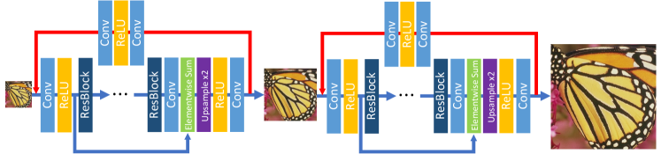
Figure 1: Demonstration of the network architectures for 4$\times$ super-resolution. The blue lines denote the standard reconstruction for the primal model and the red lines denote the backward shortcut for the dual model.

4.2 Progressive dual reconstruction for super-resolution

We build our network based on the proposed dual reconstruction scheme to exploit the mutual dependencies between LR and HR images, as shown in Figure 1. Following the design of progressive reconstructions [44, 24], the proposed model consists of multiple dual reconstruction blocks and progressively predicts the images from low-resolution to high-resolution. Let $r$ be the upscaling factor, the number of the blocks depends on the upscaling factor: $L=\log_{2}(r)$. For example, the model contains 2 blocks for 4$\times$ and 3 blocks for 8$\times$ upscaling.

The dual reconstruction scheme can be easily implemented by introducing a backward shortcut connection (see red lines in Figure 1). In each block, the primal model $P$ consists of multiple residual modules [15] followed by a sub-pixel convolution layer to increase the resolution by $2\times$ upscaling. Since the dual task aims to learn a much simpler downsampling operation compared to the primal upscaling mapping, the dual model $D$ only contains two convolution layers and a ReLU [34] activation layer. During training, we use the bicubic downsampling to resize the ground truth HR image ${\bf y}$ to ${\bf y}_{l}$ in $l$-th block. Let $\widehat{\bf y}_{l}$ be the predicted image of $l$-th block and $\widehat{\bf y}_{0}={\bf y}_{0}$ be the input LR image at the lowest level. For convenience, let $\{\theta_{P}\}$ and $\{\theta_{D}\}$ be the parameters for primal and dual models at all levels. We build a joint loss to receive the supervision at different scales:

$$\mathcal{L}(\widehat{\bf y},{\bf y};\{\theta_{P}\},\{\theta_{D}\})=\sum_{l=1}^{L}\ell_{\mathrm{DR}}(\widehat{\bf y}_{l-1},{\bf y}_{l})=\sum_{l=1}^{L}\ell_{1}\Big{(}P_{l}(\widehat{\bf y}_{l-1}),{\bf y}_{l}\Big{)}{+}\ell_{2}\Big{(}D_{l}(P_{l}(\widehat{\bf y}_{l-1})),\widehat{\bf y}_{l-1}\Big{)},$$ (7)

where $P_{l}$ and $D_{l}$ denote the primal and dual model in $l$-th block, respectively. We set both $\ell_{1}$ and $\ell_{2}$ on the primal and dual reconstruction tasks to the proposed $\ell_{\mathrm{GS}}$ loss function.

4.3 Theoretical analysis

We theoretically analyze the generalization bound for the proposed method, where all definitions, proofs and lemmas are put in Appendix A, due to the page limitation. The generalization error of the dual learning scheme is to measure how accurately the algorithm predicts for the unseen test data in the primal and dual tasks. In particular, we obtain a generalization bound of the proposed model using Rademacher complexity [4].

Theorem 1

Let $\ell_{1}(P({\bf x}),{\bf y})+\ell_{2}(D(P({\bf x})),{\bf x})$ be a mapping from ${\mathcal{X}}\times{\mathcal{Y}}$ to $[0,M]$, and the hypothesis set ${\mathcal{H}}_{dual}$ be infinite. Then, for any $\delta>0$, with probability at least $1-\delta$, the generalization error $E(P,D)$ (i.e., expected loss) satisfies for all $(P,D)\in{\mathcal{H}}_{dual}$:

$$E(P,D)\leq \widehat{E}(P,D)+2R_{m}^{DL}({\mathcal{H}}_{dual})+M\sqrt{\frac{1}{2m}\log(\frac{1}{\delta})},$$

$$E(P,D)\leq \widehat{E}(P,D)+2\widehat{R}_{{\mathcal{Z}}}^{DL}({\mathcal{H}}_{dual})+3M\sqrt{\frac{1}{2m}\log(\frac{1}{\delta})},$$

where $m$ is the sample number and $\widehat{E}(P,D)$ is the empirical loss, while $R_{m}^{DL}$ and $\widehat{R}_{{\mathcal{Z}}}^{DL}$ represent the Rademacher complexity and empirical Rademacher complexity of dual learning, respectively.

This theorem suggests that using the hypothesis set with larger capacity and more samples can guarantee better generalization. We highlight that the derived generalization bound of dual learning, where the loss function is bounded by $[0,M]$, is more general than [46].

Remark 1

Based on the definition of Rademacher complexity, the capacity of the hypothesis set ${\mathcal{H}}_{dual}{\in}{\mathcal{P}}{\times}{\mathcal{D}}$ is smaller than the capacity of hypothesis set ${\mathcal{H}}{\in}{\mathcal{P}}$ or ${\mathcal{H}}{\in}{\mathcal{D}}$ in traditional supervised learning, $i.e.$, $\widehat{R}_{{\mathcal{Z}}}^{DL}\leq\widehat{R}_{{\mathcal{Z}}}^{SL}$, where $\widehat{R}_{{\mathcal{Z}}}^{SL}$ is Rademacher complexity defined in supervised learning. In other words, dual reconstruction scheme has a smaller generalization bound than the primal feed-forward scheme and the proposed dual reconstruction model helps the primal model to achieve more accurate SR predictions.

5 Experiments

In the experiments, we perform super-resolution to recover images that are downsampled by factors of 4 and 8, respectively. We compare the performance of the proposed method with several state-of-the-art methods on five benchmark datasets, including SET5 [6], SET14 [49], BSDS100 [2], URBAN100 [17] and MANGA109 [32]. For quantitative evaluation, we adopt two common image quality metrics, i.e., PSNR and SSIM [45] in the paper.

5.1 Implementation details

We train the proposed DRN model using a random subset of 350k images from the ImageNet dataset [37]. We randomly crop the input images to $128\times 128$ RGB images as the HR data, and downsample the HR data using bicubic kernel to obtain the LR data. We use ReLU activation in both the primal and dual reconstruction model. Each reconstruction block in the primal model has $7$ identical residual modules, i.e., 14 modules for $4\times$ and 21 modules for $8\times$ upscaling. We adopt the sub-pixel convolutional layer [38] to increase the resolution by $2\times$ upscaling. The hyperparameter $\lambda$ in Eqn. (5) is set to $2$. During training, we apply the Adam algorithm [23] with $\beta_{1}=0.9$. We set minibatch size as 16. The learning rate is initialized to $10^{-5}$ and decreased by a factor of 10 for every $5\times 10^{5}$ for total $10^{6}$ iterations. All experiments were conducted using PyTorch.

Figure 2: Performance comparison of different loss functions. The PSNR and SSIM values are shown above the images. The top row denotes recovery results on gradient magnitude.

5.2 Demonstration of gradient sensitive loss

In this part, we perform super-resolution with $4\times$ upscaling to study the impacts of different losses, including the Mean Square Error (MSE), Mean Absolute Error (MAE), image gradient loss [31], and the proposed gradient-sensitive (GS) loss. Figure 2 presents the results obtained by the different losses. The top row denotes the results regarding the image gradient, and the bottom row represents the results over the RGB images. The proposed gradient-sensitive loss converges to the highest PSNR score among all the compared losses. In addition, the gradient magnitude map obtained by $\ell_{\mathrm{GS}}$ is more close to the ground-truth compared with the other losses. From the reconstructed RGB images, we observe that $\ell_{\mathrm{GS}}$ is able to capture more details and maintain the perceptual fidelity of the original HR images.

Table 1: Performance comparison with state-of-the-art algorithms for 4$\times$ upscaling image super-resolution. Bold number indicates the best result and blue number indicates the second best result.

Algorithms	SET5		SET14		BSDS100		URBAN100		MANGA109
	PSNR	SSIM	PSNR	SSIM	PSNR	SSIM	PSNR	SSIM	PSNR	SSIM
Bicubic	28.42	0.810	26.10	0.702	25.96	0.667	23.15	0.657	24.92	0.789
SRCNN [9]	30.49	0.862	27.61	0.751	26.91	0.710	24.53	0.722	27.66	0.858
SelfExSR [17]	30.33	0.861	27.54	0.751	26.84	0.710	24.82	0.737	27.82	0.865
DRCN [22]	31.53	0.885	28.04	0.767	27.24	0.723	25.14	0.751	28.97	0.886
ESPCN [38]	29.21	0.851	26.40	0.744	25.50	0.696	24.02	0.726	23.55	0.795
SRResNet [25]	32.05	0.891	28.49	0.782	27.61	0.736	26.09	0.783	30.70	0.908
SRGAN [25]	29.46	0.838	26.60	0.718	25.74	0.666	24.50	0.736	27.79	0.856
FSRCNN [10]	30.71	0.865	27.70	0.756	26.97	0.714	24.61	0.727	27.89	0.859
VDSR [21]	31.53	0.883	28.03	0.767	27.29	0.725	25.18	0.752	28.82	0.886
DRRN [40]	31.69	0.885	28.21	0.772	27.38	0.728	25.44	0.763	27.17	0.853
LapSRN [24]	31.54	0.885	28.09	0.770	27.31	0.727	25.21	0.756	29.09	0.890
SRDenseNet [42]	32.02	0.893	28.50	0.778	27.53	0.733	26.05	0.781	29.49	0.899
EDSR [28]	32.46	0.896	27.71	0.786	27.72	0.742	26.64	0.803	29.09	0.957
DBPN [13]	31.76	0.887	28.39	0.778	27.48	0.733	25.71	0.772	30.22	0.902
GS loss (ours)	32.17	0.895	28.51	0.785	27.80	0.742	25.95	0.789	30.91	0.959
DRN (ours)	32.24	0.897	28.58	0.788	27.86	0.745	26.12	0.792	30.97	0.963

5.3 Comparisons with state-of-the-art methods

We compare the performance of our proposed DRN approach with several state-of-the-art methods, including Bicubic, SRCNN [9], SelfExSR [17], DRCN [22], ESPCN [38], SRResNet [25], SRGAN [25], FSRCNN [10], VDSR [21], DRRN [40], LapSRN [24], SRDenseNet [42] and EDSR [28]. While preparing this paper, we are aware of a very recent work [13] which shows promising performance. For fair comparison, we train the model using their souce code on our data set with the same setting. However, our reproduced results are worse than the reporting results in [13]. One possible reason is that they use more training data. We study the effect of the number of training data in Figure 5 of supplementary file.

Tables 1 and 2 present the results of $4\times$ and $8\times$ image super-resolution, respectively. For the $4\times$ super-resolution tasks, our proposed GS loss and DRN approach outperform the other conducted methods on most datasets. For the $8\times$ super-resolution tasks, DRN and GS loss achieve the best and the second best performance among all the conducted methods, respectively. These observations demonstrate the effectivenes of the proposed methods. In addition, DRN with GS loss outperforms GS loss on all the datasets, which validates that the proposed dual reconstruction mechanism is able to further improve the performance. For further comparison, we provide visual comparisons on some reconstructed images. Figures 3 shows the $4\times$ and $8\times$ SR images obtained by different methods and the corresponding metrics, respectively. We observe that our proposed DRN method consistently achieves the best numerical results and the best visual quality.

Table 2: Performance comparison with state-of-the-art algorithms for 8$\times$ upscaling image super-resolution. Bold number indicates the best result and blue number indicates the second best result.

Algorithms	SET5		SET14		BSDS100		URBAN100		MANGA109
	PSNR	SSIM	PSNR	SSIM	PSNR	SSIM	PSNR	SSIM	PSNR	SSIM
Bicubic	24.39	0.657	23.19	0.568	23.67	0.547	20.74	0.515	21.47	0.649
SRCNN [9]	25.33	0.689	23.85	0.593	24.13	0.565	21.29	0.543	22.37	0.682
SelfExSR [17]	25.52	0.704	24.02	0.603	24.18	0.568	21.81	0.576	22.99	0.718
ESPCN [38]	25.02	0.697	23.45	0.598	23.92	0.574	21.20	0.554	22.04	0.683
SRResNet [25]	26.62	0.756	24.55	0.624	24.65	0.587	22.05	0.589	23.88	0.748
SRGAN [25]	23.04	0.626	21.57	0.495	21.78	0.442	19.64	0.468	20.42	0.625
FSRCNN [10]	25.41	0.682	23.93	0.592	24.21	0.567	21.32	0.537	22.39	0.672
VDSR [21]	25.72	0.711	24.21	0.609	24.37	0.576	21.54	0.560	22.83	0.707
DRRN [40]	25.76	0.721	24.21	0.583	24.47	0.533	21.02	0.530	21.88	0.663
LapSRN [24]	26.14	0.737	24.35	0.620	24.54	0.585	21.81	0.580	23.39	0.734
SRDenseNet [42]	25.99	0.704	24.23	0.581	24.45	0.530	21.67	0.562	23.09	0.712
EDSR [28]	26.54	0.752	24.54	0.625	24.59	0.588	22.07	0.595	23.74	0.749
DBPN [13]	26.43	0.748	24.39	0.623	24.60	0.589	22.01	0.592	23.97	0.756
GS loss (ours)	26.91	0.772	24.73	0.636	24.70	0.593	22.30	0.609	24.77	0.782
DRN (ours)	27.03	0.775	24.86	0.641	24.83	0.599	22.46	0.617	24.85	0.790

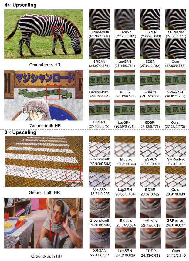
Figure 3: Visual comparison for $4\times$ and $8\times$ image super-resolution on benchmark datasets.

Table 3: Performance comparison over image gradient in terms of PSNR. [8$\times$ upscaling]

Algorithms	Set5	Set14	BSDS100	Urban100	Manga109
SRGAN [25]	20.01	19.48	19.59	18.58	19.54
SRResNet [25]	20.82	19.65	20.50	18.87	20.43
LapSRN [24]	20.14	19.29	20.36	18.48	18.96
EDSR [28]	19.84	19.31	19.98	18.39	20.16
DBPN [13]	20.93	19.76	20.47	18.87	20.50
DRN (Ours)	21.29	20.04	20.62	19.11	20.68

Table 4: Abalation study of dual reconstruction scheme and progressive structure. We report the PSNR scores on the SET5 and SET14 datasets.

Method	Plain	Dual	Progressive	Dual + Progressive
SET5	31.96	32.04	32.17	32.24
SET14	28.37	28.47	28.52	28.58

6 More results and discussions

6.1 Comparisons of PSNR over image gradient

Table 3 lists the PSNR scores over the image gradient on several benchmark datasets. Our proposed DRN achieves the best performance, which demonstrates that the DRN network has a better ability to capture the structural information compared with the other methods.

6.2 Effects of dual reconstruction scheme and progressive structure.

In this experiment, we evaluate the effects of the dual reconstruction scheme and conduct analysis on the progressive structure. The “non-progressive” methods directly predict the final HR images without the supervision from the prediction of intermediate images. The “non-dual” learning methods remove the dual learning part and fall back to plain feed-forward methods. Table 4 shows the PSNR scores of the $4\times$ super-resolution tasks on the SET5 and SET14 datasets. We observe that both the progressive and dual methods outperform the plain methods (“non-progressive” and “non-dual”) The combination of dual reconstruction scheme and progressive structure method achieves the best performance. These results demonstrate the efficacy of the proposed progressive reconstruction and dual learning approaches.

7 Conclusion

In this work, we propose a novel gradient sensitive loss (GS) to capture both low-frequency content and high-frequency structure for image super-resolution. Moreover, to exploit the mutual dependencies between LR and HR images, we propose a dual reconstruction to further improve the performance. Our model is trained with the proposed GS loss in a progressive coarse-to-fine manner. More critically, we conduct theoritical analysis on the generalization bound of the proposed method. Extensive experiments demonstrate that the proposed method produces perceptually sharper images and significantly outperforms the state-of-the-art SR methods with a large upscaling factor of $4\times$ and $8\times$.

Supplementary Materials for “Dual Reconstruction Nets for Image Super-Resolution with Gradient Sensitive Loss”

Appendix A Theoretical analysis

In this section, we will analyze the generalization bound for the proposed method. The generalization error of the dual learning scheme is to measure how accurately the algorithm predicts for the unseen test data in the primal and dual tasks. Firstly, we will introduce the definition of the generalization error as follows:

Definition 3

Given an underlying distribution ${\mathcal{S}}$ and hypotheses $P\in{\mathcal{P}}$ and $D\in{\mathcal{D}}$ for the primal and dual tasks, where ${\mathcal{P}}=\{P_{\theta_{{\bf x}{\bf y}}}({\bf x});\theta_{{\bf x}{\bf y}}\in\Theta_{{\bf x}{\bf y}}\}$ and ${\mathcal{D}}=\{D_{\theta_{{\bf y}{\bf x}}}({\bf y});\theta_{{\bf y}{\bf x}}\in\Theta_{{\bf y}{\bf x}}\}$, and $\Theta_{{\bf x}{\bf y}}$ and $\Theta_{{\bf y}{\bf x}}$ are parameter spaces, respectively, the generalization error (expected loss) of h is defined by:

$$E(P,D)={\mathbb{E}}_{({\bf x},{\bf y})\sim{\mathcal{P}}}\left[\ell_{1}(P({\bf x}),{\bf y})+\ell_{2}(D(P({\bf x})),{\bf x})\right],\;\forall P\in{\mathcal{P}},D\in{\mathcal{D}}.$$

In practice, the goal of the dual learning is to optimize the bi-directional tasks. For any $P\in{\mathcal{P}}$ and $D\in{\mathcal{D}}$, we define the empirical loss on the $m$ samples as follows:

$$\widehat{E}(P,D)=\frac{1}{m}\sum_{i=1}^{m}\ell_{1}(P({\bf x}_{i}),{\bf y}_{i})+\ell_{2}(D(P({\bf x}_{i})),{\bf x}_{i})$$ (8)

Following [4], we define Rademacher complexity for dual learning in this paper. We define the hypothesis set as ${\mathcal{H}}_{dual}\in{\mathcal{P}}\times{\mathcal{D}}$, this Rademacher complexity can measure the complexity of the hypothesis set, that is it can capture the richness of a family of the primal and the dual models. For our application, we mildly rewrite the definition of Rademacher complexity in [33] as follows:

Definition 4

(Rademacher complexity of dual learning) Given an underlying distribution ${\mathcal{S}}$, and its empirical distribution ${\mathcal{Z}}=\{{\bf z}_{1},{\bf z}_{2},\cdots,{\bf z}_{m}\}$, where ${\bf z}_{i}=({\bf x}_{i},{\bf y}_{i})$, then the Rademacher complexity of dual learning is defined as:

$$R_{m}^{DL}({\mathcal{H}}_{dual})={\mathbb{E}}_{{\mathcal{Z}}}\left[\widehat{R}_{{\mathcal{Z}}}(P,D)\right],\;\forall P\in{\mathcal{P}},D\in{\mathcal{D}},$$

where $\widehat{R}_{{\mathcal{Z}}}(P,D)$ is its empirical Rademacher complexity defined as:

$$\widehat{R}_{{\mathcal{Z}}}(P,D)={\mathbb{E}}_{\sigma}\left[\sup_{(P,D)\in{\mathcal{H}}_{dual}}\frac{1}{m}\sum_{i=1}^{m}\sigma_{i}(\ell_{1}(P({\bf x}_{i}),{\bf y}_{i})+\ell_{2}(D(P({\bf x}_{i})),{\bf x}_{i}))\right].$$

where $\sigma=\{\sigma_{1},\sigma_{2},\cdots,\sigma_{m}\}$ are independent uniform $\{\pm 1\}$-valued random variables with $p(\sigma_{i}=1)=p(\sigma_{i}=-1)=\frac{1}{2}$.

A.1 Generalization bound

This subsection give a generalization guarantees for the dual learning problem. We start with a simple case of a finite hypothesis set.

Theorem 2

Let $[\ell_{1}(P({\bf x}),{\bf y})+\ell_{2}(D(P({\bf x})),{\bf x})]$ be a mapping from ${\mathcal{X}}\times{\mathcal{Y}}$ to $[0,M]$, and suppose the hypothesis set ${\mathcal{H}}_{dual}$ is finite, then for any $\delta>0$, with probability at least $1-\delta$, the following inequality holds for all $(P,D)\in{\mathcal{H}}_{dual}$:

$$E(P,D)\leq\widehat{E}(P,D)+M\sqrt{\frac{\log|{\mathcal{H}}_{dual}|+\log\frac{1}{\delta}}{2m}}.$$

Proof 1

Based on Hoeffding’s inequality, since $[\ell_{1}(P({\bf x}),{\bf y})+\ell_{2}(D(P({\bf x})),{\bf x})]$ is bounded in $[0,M]$, for any $(P,D)\in{\mathcal{H}}_{dual}$, then

$$P\left[E(P,D)-\widehat{E}(P,D)>\epsilon\right]\leq e^{-\frac{2m\epsilon^{2}}{M^{2}}}$$

Based on the union bound, we have

$$P\left[\exists(P,D)\in{\mathcal{H}}_{dual}:E(P,D)-\widehat{E}(P,D)>\epsilon\right]$$

$$\leq \sum_{(P,D)\in{\mathcal{H}}_{dual}}P\left[E(P,D)-\widehat{E}(P,D)>\epsilon\right]$$

$$\leq |{\mathcal{H}}_{dual}|e^{-\frac{2m\epsilon^{2}}{M^{2}}}.$$

Let $|{\mathcal{H}}_{dual}|e^{-\frac{2m\epsilon^{2}}{M^{2}}}=\delta$, we have $\epsilon=M\sqrt{\frac{\log|{\mathcal{H}}_{dual}|+\log\frac{1}{\delta}}{2m}}$ and conclude the theorem.

This theorem shows that a larger sample size $m$ and smaller hypothesis set can guarantee the generalization. Next we will give a generalization bound of a general case of infinite hypothesis sets using Rademacher complexity.

Theorem 3

Let $\ell_{1}(P({\bf x}),{\bf y})+\ell_{2}(D(P({\bf x})),{\bf x})$ be a mapping from ${\mathcal{X}}\times{\mathcal{Y}}$ to $[0,M]$, then for any $\delta>0$, with probability at least $1-\delta$, the following inequality holds for all $(P,D)\in{\mathcal{H}}_{dual}$:

$$E(P,D)\leq \widehat{E}(P,D)+2R_{m}^{DL}+M\sqrt{\frac{1}{2m}\log(\frac{1}{\delta})}$$ (9)

$$E(P,D)\leq \widehat{E}(P,D)+2\widehat{R}_{{\mathcal{Z}}}^{DL}+3M\sqrt{\frac{1}{2m}\log(\frac{1}{\delta})}.$$ (10)

Proof 2

Based on Theorem 3.1 in [33], we extend a case for $\ell_{1}(P({\bf x}),{\bf y})+\ell_{2}(D(P({\bf x})),{\bf x})$ bounded in $[0,M]$.

Theorem 3 shows that with probability at least $1-\delta$, the generalization error is smaller than $2R_{m}^{DL}+M\sqrt{\frac{1}{2m}\log(\frac{1}{\delta})}$ or $2\widehat{R}_{{\mathcal{Z}}}^{DL}+3M\sqrt{\frac{1}{2m}\log(\frac{1}{\delta})}$. It suggests that using the hypothesis set with larger capacity and more samples can guarantee better generalization. Moreover, the generalization bound of dual learning is more general for the case that the loss function $\ell_{1}(P({\bf x}),{\bf y})+\ell_{2}(D(P({\bf x})),{\bf x})$ is bounded by $[0,M]$, which is different from [46].

Remark 2

Based on the definition of Rademacher complexity, the capacity of the hypothesis set ${\mathcal{H}}_{dual}{\in}{\mathcal{P}}{\times}{\mathcal{D}}$ is smaller than the capacity of hypothesis set ${\mathcal{H}}{\in}{\mathcal{P}}$ or ${\mathcal{H}}{\in}{\mathcal{D}}$ in traditional supervised learning, $i.e.$, $\widehat{R}_{{\mathcal{Z}}}^{DL}\leq\widehat{R}_{{\mathcal{Z}}}^{SL}$, where $\widehat{R}_{{\mathcal{Z}}}^{SL}$ is Rademacher complexity defined in supervised learning. In other words, dual learning has a smaller generalization bound than supervised learning and the proposed dual reconstruction model helps the primal model to achieve more accurate SR predictions.

Appendix B Discussions

B.1 Demonstration of gradient sensitive loss

For better understanding, we plot some results about our manipulation of image gradient in Figure 4. By visualizing the gradient $\nabla\mathbf{I}$ of the image $\mathbf{I}$, we can observe the structure information directly. Meanwhile, $\mathbf{M}\odot\mathbf{I}$ means the mask $\mathbf{M}$ has the pixel-wise multiplication with image $\mathbf{I}$ and $(\mathbf{1}-\mathbf{M})\odot\mathbf{I}$ represent the rest part. In our proposed method, we use the gradient of $\mathbf{M}\odot\mathbf{I}$, i.e. $\nabla(\mathbf{M}\odot\mathbf{I})$, to compute the loss function.

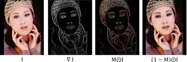
Figure 4: Demonstration of the mask ${\bf M}$.

B.2 Comparisons of different loss functions and training schemes

Table 5 summarizes the characteristics of different loss functions and training schemes. In particular, the standard training scheme only forces the model to match the HR images, while the dual scheme receives the supervised information from both LR and HR images.

For the different objective functions, the perceptual loss does not obtain frequency information from images, the gradient loss only captures the high-frequency information, and the MAE, MSE and adversarial loss only btains the low-frequency information. In comparison, our proposed gradient-sensitive loss ($\ell_{\mathrm{GS}}$) is able to capture both the low- and high-frequency information from images.

Overall, the proposed DRN method with the dual scheme is able to exploit both the low- and high-frequency information, and receive supervision form both LR and HR images.

Table 5: Comparisons of different objectives and training schemes in Super-Resolution. $\checkmark$ denotes YES, while blank denotes NO.

Schemes	Methods	Supervision		Information
		LR images	HR images	low-frequency	high-frequency
Standard	MAE		✓	✓
	MSE		✓	✓
	Gradient loss		✓		✓
	Adversarial loss		✓	✓
	Percputal loss		✓
	$\ell_{\mathrm{GS}}$ loss (ours)		✓	✓	✓
Dual	$\ell_{\mathrm{GS}}$ loss (ours)	✓	✓	✓	✓

Appendix C Experimental results

C.1 Effect of $\lambda$ in Eqn. (5)

In this experiment, we study the performance of our proposed DRN method under different values of the parameter $\lambda$. From Table 6, when the parameter $\lambda$ is too small, the method cannot achieve promising performance, since the gradient-level loss only captures the structural information. When the parameter $\lambda$ increases monotonically, the performance of DRN increases gradually. This demonstrates that the combination of the gradient-level loss and the pixel-level loss is effective to achieve promising results. In our setting, we empirically set $\lambda=2$, since we find that a larger value usually does not bring further performance improvement.

Table 6: Performance w.r.t. different values of $\lambda$.

$\lambda$	0.1	0.5	1.0	1.5	2.0	5.0
PSNR	30.44	31.55	31.92	32.13	32.24	32.24

C.2 Effect of training data ratio

We conduct an experiment on SET5 to evaluate the influence of the number of training data. From Figure 5, when increasing the ratio of training data on the whole dataset, the values of PSNR score increases gradually. In addition, DRN consistently outperforms DBPN on all the data ratios.

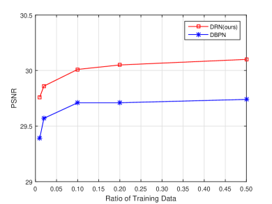
Figure 5: The results in different magnitude of ImageNet dataset.

C.3 Comparison of model complexity

We report the PSNR scores and the numbers of the parameters in DRN and several state-of-the-art models on $4\times$ and $8\times$ SR in Figures 6 and 7, respectively. The x-axis represents the number of the model parameters, and the y-axis means the value of PSNR. The results show that the proposed DRN method can achieve the best performance on both two datasets with the lowest computational complexity compared with the other baseline methods.

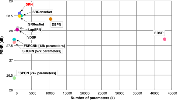
Figure 6: The results for $4\times$ SR on SET14 dataset.

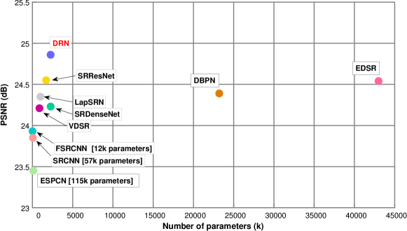
Figure 7: The results for $8\times$ SR on SET14 dataset.

C.4 More results

For further comparison, we provide the experimental results compared with the baseline methods for $8\times$ SR on several benchmark datasets.

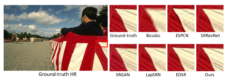
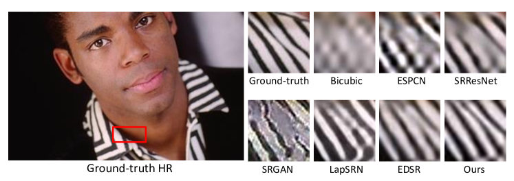
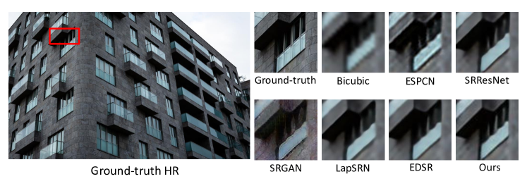
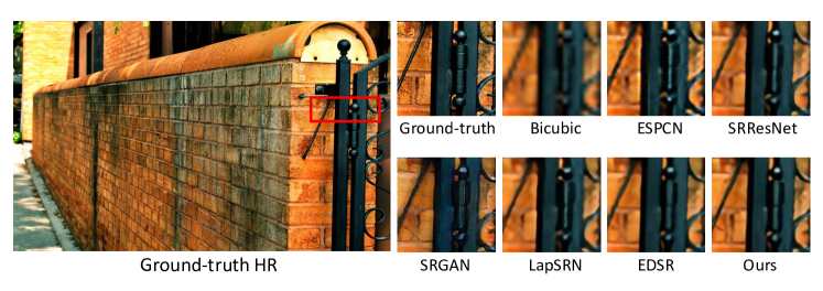
Figure 8: More results of visual comparison for $8\times$ upscaling super-resolution.

References

- [1] Jan Allebach and Ping Wah Wong. Edge-directed interpolation. In Image Processing, 1996. Proceedings., International Conference on, volume 3, pages 707–710. IEEE, 1996.
- [2] Pablo Arbelaez, Michael Maire, Charless Fowlkes, and Jitendra Malik. Contour detection and hierarchical image segmentation. IEEE transactions on pattern analysis and machine intelligence, 33(5):898–916, 2011.
- [3] Simon Baker and Takeo Kanade. Limits on super-resolution and how to break them. IEEE Transactions on Pattern Analysis and Machine Intelligence, 24(9):1167–1183, 2002.
- [4] Peter L Bartlett and Shahar Mendelson. Rademacher and gaussian complexities: Risk bounds and structural results. Journal of Machine Learning Research, 3(Nov):463–482, 2002.
- [5] Moshe Ben-Ezra, Zhouchen Lin, and Bennett Wilburn. Penrose pixels super-resolution in the detector layout domain. In Computer Vision, 2007. ICCV 2007. IEEE 11th International Conference on, pages 1–8. IEEE, 2007.
- [6] Marco Bevilacqua, Aline Roumy, Christine Guillemot, and Marie Line Alberi-Morel. Low-complexity single-image super-resolution based on nonnegative neighbor embedding. 2012.
- [7] Debabrata Chowdhuri, KS Sendhil Kumar, M Rajasekhara Babu, and Ch Pradeep Reddy. Very low resolution face recognition in parallel environment. IJCSIT) International Journal of Computer Science and Information Technologies, 3(3):4408–4410, 2012.
- [8] Chao Dong, Chen Change Loy, Kaiming He, and Xiaoou Tang. Learning a deep convolutional network for image super-resolution. In European Conference on Computer Vision, pages 184–199. Springer, 2014.
- [9] Chao Dong, Chen Change Loy, Kaiming He, and Xiaoou Tang. Image Super-resolution using Deep Convolutional Networks. IEEE transactions on pattern analysis and machine intelligence, 38(2):295–307, 2016.
- [10] Chao Dong, Chen Change Loy, and Xiaoou Tang. Accelerating the super-resolution convolutional neural network. In European Conference on Computer Vision, pages 391–407. Springer, 2016.
- [11] Xinbo Gao, Kaibing Zhang, Dacheng Tao, and Xuelong Li. Image super-resolution with sparse neighbor embedding. IEEE Transactions on Image Processing, 21(7):3194–3205, 2012.
- [12] Shuhang Gu, Wangmeng Zuo, Qi Xie, Deyu Meng, Xiangchu Feng, and Lei Zhang. Convolutional sparse coding for image super-resolution. In Proceedings of the IEEE International Conference on Computer Vision, pages 1823–1831, 2015.
- [13] Muhammad Haris, Greg Shakhnarovich, and Norimichi Ukita. Deep back-projection networks for super-resolution. 2018.
- [14] Di He, Yingce Xia, Tao Qin, Liwei Wang, Nenghai Yu, Tieyan Liu, and Wei-Ying Ma. Dual learning for machine translation. In Advances in Neural Information Processing Systems, pages 820–828, 2016.
- [15] Kaiming He, Xiangyu Zhang, Shaoqing Ren, and Jian Sun. Deep Residual Learning for Image Recognition. In Proceedings of the IEEE Conference on Computer Vision and Pattern Recognition, pages 770–778, 2016.
- [16] Hsieh Hou and H Andrews. Cubic splines for image interpolation and digital filtering. IEEE Transactions on acoustics, speech, and signal processing, 26(6):508–517, 1978.
- [17] Jia-Bin Huang, Abhishek Singh, and Narendra Ahuja. Single image super-resolution from transformed self-exemplars. In Proceedings of the IEEE Conference on Computer Vision and Pattern Recognition, pages 5197–5206, 2015.
- [18] Zheng Hui, Xiumei Wang, and Xinbo Gao. Fast and accurate single image super-resolution via information distillation network. IEEE Conference on Computer Vision and Pattern Recognition (CVPR), 2018.
- [19] Yang Jianchao, John Wright, Thomas Huang, and Yi Ma. Image super-resolution as sparse representation of raw image patches. In Proc. IEEE Conf. on Computer Vision and Pattern Recognition, pages 1–8, 2008.
- [20] Justin Johnson, Alexandre Alahi, and Li Fei-Fei. Perceptual Losses for Real-time Style Transfer and Super-resolution. In European Conference on Computer Vision, pages 694–711. Springer, 2016.
- [21] Jiwon Kim, Jung Kwon Lee, and Kyoung Mu Lee. Accurate image super-resolution using very deep convolutional networks. In Proceedings of the IEEE Conference on Computer Vision and Pattern Recognition, pages 1646–1654, 2016.
- [22] Jiwon Kim, Jung Kwon Lee, and Kyoung Mu Lee. Deeply-recursive convolutional network for image super-resolution. In Proceedings of the IEEE conference on computer vision and pattern recognition, pages 1637–1645, 2016.
- [23] Diederik Kingma and Jimmy Ba. Adam: A method for stochastic optimization. International Conference on Learning Representations, 2015.
- [24] Wei-Sheng Lai, Jia-Bin Huang, Narendra Ahuja, and Ming-Hsuan Yang. Deep laplacian pyramid networks for fast and accurate super-resolution. In Proc. IEEE Conf. Comput. Vis. Pattern Recognit., pages 624–632, 2017.
- [25] Christian Ledig, Lucas Theis, Ferenc Huszár, Jose Caballero, Andrew Cunningham, Alejandro Acosta, Andrew Aitken, Alykhan Tejani, Johannes Totz, Zehan Wang, et al. Photo-realistic Single Image Super-resolution using a Generative Adversarial Network. IEEE Conference on Computer Vision and Pattern Recognition (CVPR), 2017.
- [26] Xin Li and Michael T Orchard. New edge-directed interpolation. IEEE transactions on image processing, 10(10):1521–1527, 2001.
- [27] Renjie Liao, Xin Tao, Ruiyu Li, Ziyang Ma, and Jiaya Jia. Video super-resolution via deep draft-ensemble learning. In Proceedings of the IEEE International Conference on Computer Vision, pages 531–539, 2015.
- [28] Bee Lim, Sanghyun Son, Heewon Kim, Seungjun Nah, and Kyoung Mu Lee. Enhanced deep residual networks for single image super-resolution. In The IEEE Conference on Computer Vision and Pattern Recognition (CVPR) Workshops, volume 1, page 3, 2017.
- [29] Zhouchen Lin and Heung-Yeung Shum. Fundamental limits of reconstruction-based superresolution algorithms under local translation. IEEE Transactions on Pattern Analysis and Machine Intelligence, 26(1):83–97, 2004.
- [30] Xiaojiao Mao, Chunhua Shen, and Yu-Bin Yang. Image restoration using very deep convolutional encoder-decoder networks with symmetric skip connections. In D. D. Lee, M. Sugiyama, U. V. Luxburg, I. Guyon, and R. Garnett, editors, Advances in Neural Information Processing Systems 29, pages 2802–2810. Curran Associates, Inc., 2016.
- [31] Michael Mathieu, Camille Couprie, and Yann LeCun. Deep Multi-scale Video Prediction beyond Mean Square Error. International Conference on Learning Representations, 2016.
- [32] Yusuke Matsui, Kota Ito, Yuji Aramaki, Azuma Fujimoto, Toru Ogawa, Toshihiko Yamasaki, and Kiyoharu Aizawa. Sketch-based manga retrieval using manga109 dataset. Multimedia Tools and Applications, 76(20):21811–21838, 2017.
- [33] Mehryar Mohri, Afshin Rostamizadeh, and Ameet Talwalkar. Foundations of machine learning. MIT press, 2012.
- [34] Vinod Nair and Geoffrey E Hinton. Rectified linear units improve restricted boltzmann machines. In Proceedings of the 27th international conference on machine learning (ICML-10), pages 807–814, 2010.
- [35] Elias Nehme, Lucien E Weiss, Tomer Michaeli, and Yoav Shechtman. Deep-storm: super-resolution single-molecule microscopy by deep learning. Optica, 5(4):458–464, 2018.
- [36] Nhat Nguyen and Peyman Milanfar. An efficient wavelet-based algorithm for image superresolution. In Image Processing, 2000. Proceedings. 2000 International Conference on, volume 2, pages 351–354. IEEE, 2000.
- [37] Olga Russakovsky, Jia Deng, Hao Su, Jonathan Krause, Sanjeev Satheesh, Sean Ma, Zhiheng Huang, Andrej Karpathy, Aditya Khosla, Michael Bernstein, et al. Imagenet Large Scale Visual Recognition Challenge. International Journal of Computer Vision, 115(3):211–252, 2015.
- [38] Wenzhe Shi, Jose Caballero, Ferenc Huszár, Johannes Totz, Andrew P Aitken, Rob Bishop, Daniel Rueckert, and Zehan Wang. Real-time Single Image and Video Super-resolution using an Efficient Sub-pixel Convolutional Neural Network. In Proceedings of the IEEE Conference on Computer Vision and Pattern Recognition, pages 1874–1883, 2016.
- [39] Karen Simonyan and Andrew Zisserman. Very deep convolutional networks for large-scale image recognition. arXiv preprint arXiv:1409.1556, 2014.
- [40] Ying Tai, Jian Yang, and Xiaoming Liu. Image super-resolution via deep recursive residual network. In The IEEE Conference on Computer Vision and Pattern Recognition (CVPR), volume 1, 2017.
- [41] Radu Timofte, Vincent De, and Luc Van Gool. Anchored neighborhood regression for fast example-based super-resolution. In Computer Vision (ICCV), 2013 IEEE International Conference on, pages 1920–1927. IEEE, 2013.
- [42] Tong Tong, Gen Li, Xiejie Liu, and Qinquan Gao. Image super-resolution using dense skip connections. In 2017 IEEE International Conference on Computer Vision (ICCV), pages 4809–4817. IEEE, 2017.
- [43] Xintao Wang, Ke Yu, Chao Dong, and Chen Change Loy. Recovering realistic texture in image super-resolution by deep spatial feature transform. IEEE Conference on Computer Vision and Pattern Recognition (CVPR), 2018.
- [44] Zhaowen Wang, Ding Liu, Jianchao Yang, Wei Han, and Thomas Huang. Deep networks for image super-resolution with sparse prior. In Proceedings of the IEEE International Conference on Computer Vision, pages 370–378, 2015.
- [45] Zhou Wang, Alan C Bovik, Hamid R Sheikh, and Eero P Simoncelli. Image quality assessment: from error visibility to structural similarity. IEEE transactions on image processing, 13(4):600–612, 2004.
- [46] Yingce Xia, Tao Qin, Wei Chen, Jiang Bian, Nenghai Yu, and Tie-Yan Liu. Dual supervised learning. In Doina Precup and Yee Whye Teh, editors, Proceedings of the 34th International Conference on Machine Learning, volume 70 of Proceedings of Machine Learning Research, pages 3789–3798, International Convention Centre, Sydney, Australia, 06–11 Aug 2017. PMLR.
- [47] Yingce Xia, Tao Qin, Wei Chen, Jiang Bian, Nenghai Yu, and Tie-Yan Liu. Dual supervised learning. arXiv preprint arXiv:1707.00415, 2017.
- [48] Chih-Yuan Yang, Chao Ma, and Ming-Hsuan Yang. Single-image super-resolution: A benchmark. In European Conference on Computer Vision, pages 372–386. Springer, 2014.
- [49] Roman Zeyde, Michael Elad, and Matan Protter. On single image scale-up using sparse-representations. In International conference on curves and surfaces, pages 711–730. Springer, 2010.
- [50] Kai Zhang, Wangmeng Zuo, and Lei Zhang. Learning a single convolutional super-resolution network for multiple degradations. IEEE Conference on Computer Vision and Pattern Recognition (CVPR), 2018.
- [51] Yulun Zhang, Yapeng Tian, Yu Kong, Bineng Zhong, and Yun Fu. Residual dense network for image super-resolution. IEEE Conference on Computer Vision and Pattern Recognition (CVPR), 2018.