Ultrafast Calculation of Diffuse Scattering from Atomistic Models

Abstract

Diffuse scattering is a rich source of information about disorder in crystalline materials, which can be modelled using atomistic techniques such as Monte Carlo and molecular dynamics simulations. Modern X-ray and neutron scattering instruments can rapidly measure large volumes of diffuse-scattering data. Unfortunately, current algorithms for atomistic diffuse-scattering calculations are too slow to model large data sets completely, because the fast Fourier transform (FFT) algorithm has long been considered unsuitable for such calculations Butler_1992 . Here, I present a new approach for ultrafast calculation of atomistic diffuse-scattering patterns. I show that the FFT can be actually be used to perform such calculations rapidly, and that a fast method based on sampling theory can be used to reduce high-frequency noise in the calculations. I benchmark these algorithms using realistic examples of compositional, magnetic, and displacive disorder. They accelerate the calculations by a factor of at least 100, making refinement of atomistic models to large diffuse-scattering volumes practical.

I Introduction

Disorder plays an increasingly important role in our understanding of crystalline materials. Whereas conventional crystallography is primarily concerned with the average positions of atoms or molecules, local deviations from the average structure are fundamental to the properties of many important systems. Topical examples include fast-ion conductors Keen_2002 , frustrated magnets Fennell_2009 ; Paddison_2013a , the polar nanodomains of lead-based perovskite ferroelectrics Xu_2004 ; Pasciak_2012 , and the orbital correlations of colossal magnetoresistance manganites Shimomura_1999 . Diffuse scattering—the weak features observed beneath and between the Bragg peaks in scattering experiments—plays a central role in helping us to understand structural disorder Billinge_2007 . Whereas Bragg peaks arise from the ideal periodicity of the average structure and yield information about single-particle correlations, diffuse scattering arises from local deviations from the average structure and yields information about pairwise correlations. In disordered crystals, strong pairwise correlations are often present at the nanoscale, yielding highly-structured diffuse-scattering patterns Keen_2015 ; Overy_2016 ; Weber_2012 . Disorder in crystalline materials can often be divided into three broad categories: local atomic displacements, which may be either static or dynamic; local variations in chemical composition such as site mixing and atomic vacancies; and disordered spin arrangements in magnetic materials. In all cases, the modulation of the diffuse-scattering intensity provides vital information about how the relevant degrees of freedom—whether displacive, compositional, or magnetic—are locally correlated.

Recent advances in instrumentation have allowed rapid collection of large three-dimensional (3D) diffuse-scattering datasets from single crystals. In neutron-scattering experiments, such datasets can be measured in a matter of days using time-of-flight instruments with large detector coverage, such as SXD at the ISIS Neutron Source Keen_2006 and Corelli at the Oak Ridge National Laboratory Ye_2018 . In X-ray scattering experiments, single-photon-counting area detectors such as the Pilatus Kraft_2009 allow such datasets to be obtained in minutes. These experimental developments have been coupled with advances in 3D atomistic modelling. Atomistic models may be generated using Monte Carlo or molecular dynamics simulations based on a set of interaction parameters, which are determined either from first-principles simulations Gutmann_2013 or by fitting to experimental data Welberry_1998 ; Welberry_2008 ; Weber_2002 . Alternatively, atomistic models may be generated by fitting atomic positions or magnetic-moment orientations directly to experimental data, in an approach called reverse Monte Carlo refinement McGreevy_1988 ; Tucker_2007 ; Paddison_2012 . Improvements in computing power have greatly reduced the time required to generate atomistic models using these approaches.

A key step in atomistic diffuse-scattering analysis is calculating the diffuse-scattering intensity, which must usually be repeated several times as the model is improved. In principle, this involves the straightforward procedure of taking the Fourier transform of a set of atomic positions. In practice, however, such calculations are limitingly slow, because of two main problems. The first problem is that the fast Fourier transform (FFT) algorithm—which can yield enormous increases in speed compared to direct Fourier summation—has been considered unsuitable for these calculations Butler_1992 . This is because the FFT requires sampling atomic positions on an equally-spaced grid Cooley_1965 , but a grid that sampled local atomic displacements accurately would need so many samples that the computational advantages of the FFT would be negated Butler_1992 ; Neder_1989 ; Rahman_1989 . The second problem is that diffuse-scattering calculations are often marred by high-frequency noise. This occurs because the entire atomistic model is assumed to scatter coherently, which often allows the many essentially-uncorrelated atomic displacements at large interatomic distances to dominate the calculation Butler_1992 . Current software addresses this problem by dividing the supercell into many smaller regions called “sub-boxes” or “lots” and averaging the scattering intensity over sub-boxes Butler_1992 ; Proffen_1997 . This approach is effective at reducing noise, but has a large computational cost that can only be reduced by parallelization Gutmann_2010 . Because of their computational cost, diffuse-scattering calculations have typically been restricted to a few 2D sections of reciprocal space Welberry_2008 . In most cases, therefore, the information content of 3D diffuse-scattering data has yet to be fully explored.

Here, I present an approach to diffuse-scattering calculations that seeks to address the computational limitations of current algorithms. I present two main results. First, I critically reassess the assumption that the FFT is not useful for atomistic diffuse-scattering calculations. I show that, on the contrary, the FFT can be used to perform such calculations rapidly. This FFT-based approach is exact for systems in which the disorder is compositional, magnetic, or in which atomic displacements are drawn from a discrete set of values; if atomic displacements can take a continuous range of values, then the FFT can be applied to a specified order of approximation. Second, I show that the desirable noise-reduction properties of the “sub-box” approach can also be obtained by a faster method based on sampling theory. I demonstrate the practicality of these algorithms by presenting example calculations based on real materials, and by providing a program Scatty for ultrafast diffuse-scattering calculations [27]. These developments accelerate atomistic diffuse-scattering calculations by several orders of magnitude compared to current algorithms, making refinement of atomistic models to 3D diffuse-scattering data a practical possibility.

This article is structured as follows. In Section II, I review the scattering equations and aspects of sampling theory in the context of atomistic models. In Section III, I show how the FFT can be used to accelerate atomistic diffuse-scattering calculations. In Section IV, I present example calculations for model systems that exhibit occupational, magnetic, and displacive disorder, in which highly-structured diffuse scattering is driven by “ice rules”. In Section V, I show how noise in the calculations can be reduced using a resampling approach. I conclude in Section VI with a discussion of the implications of this work.

II Atomistic simulations

In atomistic simulations, disorder is modelled using a “virtual crystal”. This is a supercell of the crystallographic unit cell, typically containing $N\sim 10^{4}$ atomic positions, in which each atomic position is decorated by variables corresponding to its occupancy by a certain element, its displacement from its average position, and/or the orientation of its magnetic moment. I consider a supercell that consists of $n_{1}n_{2}n_{3}$ crystallographic unit cells, where $n_{1}$, $n_{2}$, and $n_{3}$ are the numbers of unit cells parallel to the $\mathbf{a},\mathbf{b}$, and $\mathbf{c}$ crystal axes, respectively. An atomic position in the supercell is given by

$$\mathbf{r}=n_{1}r_{1}\mathbf{a}+n_{2}r_{2}\mathbf{b}+n_{3}r_{3}\mathbf{c};\quad 0\leq r_{\alpha}<1.$$ (1)

An interatomic vector is denoted $\Delta\mathbf{r}$, with components $\Delta r_{\alpha}$. A general wavevector is given by

$$\mathbf{Q} =h\mathbf{a}^{*}+k\mathbf{b}^{*}+l\mathbf{c}^{*}$$ (2)

$$\equiv\frac{Q_{1}}{n_{1}}\mathbf{a}^{*}+\frac{Q_{2}}{n_{2}}\mathbf{b}^{*}+\frac{Q_{3}}{n_{3}}\mathbf{c}^{*};\quad Q_{\alpha}\in\mathbb{R},$$ (3)

where reciprocal-lattice vectors are defined as $\mathbf{a}^{*}=2\pi\mathbf{b}\times\mathbf{c}/V$, etc., where $V$ is the unit-cell volume. Atomistic simulations usually impose periodic boundary conditions to avoid edge effects, and I assume throughout this article that this is the case. The Bragg positions of the periodic supercell are then given by

$$\mathbf{G} =\frac{G_{1}}{n_{1}}\mathbf{a}^{*}+\frac{G_{2}}{n_{2}}\mathbf{b}^{*}+\frac{G_{3}}{n_{3}}\mathbf{c}^{*};\quad G_{\alpha}\in\mathbb{Z},$$ (4)

and become increasingly closely spaced as the number of unit cells in the supercell is increased.

The coherent neutron-scattering intensity from a real crystal is given, in the kinematic approximation, by

$$I(\mathbf{Q}) =\frac{1}{N}\sum_{j,k}\left\langle b_{j}b_{k}\exp\left[\mathrm{i}\mathbf{Q}\cdot(\mathbf{r}_{j}-\mathbf{r}_{k})\right]\right\rangle$$ (5)

$$\equiv\sum_{\Delta\mathbf{r}}\rho(\Delta\mathbf{r})\exp(\mathrm{i}\mathbf{Q}\cdot\Delta\mathbf{r}),$$ (6)

where $b_{j}$ is the coherent neutron scattering length of atom $j$, and $\rho(\Delta\mathbf{r})=\frac{1}{N}\sum_{j,k}\left\langle b_{j}b_{k}\delta_{\Delta\mathbf{r},\mathbf{r}_{j}-\mathbf{r}_{k}}\right\rangle$ is the 3D pair-distribution function Weber_2012 . Angle brackets denote spatial and temporal averaging, which can be approximated in atomistic modelling by averaging over many supercells. For X-ray scattering, the $b_{j}$ are replaced by $|\mathbf{Q}|$-dependent X-ray form factors, $f_{j}(|\mathbf{Q}|)$. Conventional diffraction measurements do not resolve the energy of the scattered beam and therefore integrate over energy; this integration is complete provided that the incident radiation energy significantly exceeds the energy of structural fluctuations in the sample. The $\rho(\Delta\mathbf{r})$ obtained from energy-integrated data is the correlation function of the instantaneous (equal-time) atomic positions Egami_2003 , and atomistic models of energy-integrated data similarly function as “snapshots” of the instantaneous atomic positions Goodwin_2004 .

By factorizing the double summation in Eq. (5), the scattering intensity can be rewritten as

$$I(\mathbf{Q})=\frac{1}{N}\left\langle|F(\mathbf{Q})|^{2}\right\rangle,$$ (7)

where the structure factor is a discrete Fourier transform,

$$F(\mathbf{Q})=\sum_{j=1}^{N}b_{j}\exp(\mathrm{i}\mathbf{Q}\cdot\mathbf{r}_{j}).$$ (8)

In general, the scattering intensity from a disordered crystal can be separated into its Bragg and diffuse contributions,

$$I(\mathbf{Q}) =I_{\mathrm{Bragg}}(\mathbf{Q})+I_{\mathrm{diffuse}}(\mathbf{Q}),$$ (9)

$$=\frac{1}{N}\left|\left\langle F(\mathbf{Q})\right\rangle\right|^{2}+\frac{1}{N}\left\langle\left|F(\mathbf{Q})-\left\langle F(\mathbf{Q})\right\rangle\right|^{2}\right\rangle,$$ (10)

which arise from the average structure and local modulations away from the average, respectively Frey_1997 .

Atomistic models inevitably contain far fewer unit cells ($\sim$$10^{3}$) than do real crystals ($\sim$$10^{23}$), and it is important to consider how this affects scattering calculations. Fundamentally, a periodic supercell only contains information about pair correlations for which $-r_{\mathrm{cut}}\leq\Delta r_{\alpha}<r_{\mathrm{cut}}$, where $r_{\mathrm{cut}}=0.5$. Scattering calculations may account for this in two different ways. First, if the scattering is calculated using Eq. (5), then the separation between pairs is taken to be the shortest separation between their periodic images; this is called the nearest-image convention and involves replacing $\Delta r_{\alpha}$ with $\Delta r_{\alpha}\pm 1$ where necessary to ensure $-r_{\mathrm{cut}}\leq\Delta r_{\alpha}<r_{\mathrm{cut}}$. This procedure can be conceptualized as multiplying the pair-distribution function for an infinite tiling of the supercell, $\rho_{\mathrm{inf}}(\Delta r_{\alpha})$, by a cutoff function, so that

$$\rho(\Delta r_{\alpha})=\rho_{\mathrm{inf}}(\Delta r_{\alpha})\times\mathrm{cutoff}(\Delta r_{\alpha}),$$ (11)

where $\mathrm{cutoff}(\Delta r_{\alpha})$ is a rectangular function equal to $1$ for $-r_{\mathrm{cut}}\leq\Delta r_{\alpha}<r_{\mathrm{cut}}$ and zero elsewhere. In this case, the calculated $I(\mathbf{Q})$ is a smooth function of wavevector, which contains finite-size artifacts because the contribution of the average structure to $\rho_{\mathrm{inf}}(\Delta r_{\alpha})$ is truncated. In contrast, $I_{\mathrm{diffuse}}(\mathbf{Q})$ is free from finite-size artifacts provided that the local modulations are short-ranged compared to $r_{\mathrm{cut}}$. The second approach is to calculate the scattering using Eqs. (7) and (8). In this case, the nearest-image convention cannot be applied. Consequently, the scattering intensity may only be sampled at the supercell Bragg positions $\{\mathbf{G}\}$, for which $I(\mathbf{G})$ is unchanged by the nearest-image convention because $\exp(\pm\mathrm{i}\mathbf{G}\cdot\mathbf{n})=1$. The two approaches become equivalent for real crystals, which are large enough that the boundary conditions become irrelevant.

In practice, it is much faster to calculate the scattering intensity using Eqs. (7) and (8)—which require only a single summation over atomic positions—than to use Eq. (5), which requires a double summation. However, the resulting limitation that only $I(\mathbf{G})$ may be calculated is often too restrictive, especially when a direct comparison with experimental data is required Butler_1992 . To solve this problem, I consider the information content of the scattering pattern. Applying the convolution theorem to Eq. (11) yields

$$I(\mathbf{Q}) =\sum_{\mathbf{G}=-\infty}^{\infty}I(\mathbf{G})W_{\mathrm{sinc}}(\mathbf{Q}-\mathbf{G}),$$ (12)

where the weight function

$$W_{\mathrm{sinc}}(\mathbf{Q}-\mathbf{G}) =8r_{\mathrm{cut}}^{3}\prod_{\alpha=1}^{3}\textrm{sinc}\left[2\pi r_{\mathrm{cut}}(Q_{\alpha}-G_{\alpha})\right]$$ (13)

is the Fourier transform of the rectangular function, $I(\mathbf{G})$ is the Fourier transform of $\rho_{\mathrm{inf}}(\Delta\mathbf{r})$ sampled at $\{\mathbf{G}\}$, and $\mathrm{sinc}(x)=\sin(x)/x$ Whittaker_1915 ; Shannon_1949 . In the context of sampling theory, Eqs. (12) and (13) are known as the Whittaker-Shannon interpolation formulae. They show that the scattering intensity can, in principle, be reconstructed at any wavevector $\mathbf{Q}$, given only its samples at the supercell Bragg positions $\{\mathbf{G}\}$. This is possible because the supercell Bragg positions sample $I(\mathbf{Q})$ at its Nyquist rate Sayre_1952 .

In the rest of this article, I will first show how $I(\mathbf{G})$ can be calculated rapidly using the FFT algorithm. I will then show how $I(\mathbf{Q})$ can be estimated in practice, by modifying Eqs. (12) and (13).

III Fast Fourier transform

III.1 Requirements for the FFT

The FFT is an algorithm that calculates the discrete Fourier transform rapidly Cooley_1965 ; Singleton_1969 . In the 3D case relevant for crystalline materials, it calculates a function of the form

$$X_{\mathbf{k}} =\sum_{\mathbf{R}}x_{\mathbf{R}}\exp(\mathrm{i}\mathbf{k}\cdot\mathbf{R}).$$ (14)

Unlike the discrete Fourier transform, for which the position vector $\mathbf{R}$ and wavevector $\mathbf{k}$ can take any real values, the FFT imposes two restrictions. First, the $x_{\mathbf{R}}$ must be arranged on an equally-spaced grid, so that

$$\mathbf{R}=R_{1}\mathbf{a}+R_{2}\mathbf{b}+R_{3}\mathbf{c};~{}R_{\alpha}\in\left\{0,1,...,N_{\alpha}-1\right\},$$ (15)

where $N_{\alpha}$ denotes the number of grid points parallel to crystal axis $\alpha$ in the supercell. Second, the values of $\mathbf{k}$ at which the Fourier coefficients $X_{\mathbf{k}}$ may be evaluated are given by

$$\mathbf{k}=\frac{k_{1}}{N_{1}}\mathbf{a}^{\ast}+\frac{k_{2}}{N_{2}}\mathbf{b}^{\ast}+\frac{k_{3}}{N_{3}}\mathbf{c}^{\ast};\quad k_{\alpha}\in\left\{0,1,...,N_{\alpha}-1\right\}.$$ (16)

Below, I will identify the grid points with lattice points, so that $N_{\alpha}=n_{\alpha}$ and each grid point is the origin of a particular unit cell within the supercell. In this case, the values of $\mathbf{k}$ given by Eq. (16) are a subset of the supercell Bragg positions that lie within a fundamental domain of the reciprocal lattice of the supercell.

The computational cost of the discrete Fourier transform is on the order of $\left(N_{1}N_{2}N_{3}\right)^{2}$, whereas for the FFT it is on the order of $N_{1}N_{2}N_{3}\log_{2}(N_{1}N_{2}N_{3})$—a huge saving for large $N_{1}N_{2}N_{3}$. Unfortunately, the atomic positions in a crystal do not generally satisfy Eq. (15), except in the special case where atoms occupy a Bravais lattice without disorder. In early work, it was assumed that this restriction could only be addressed by using a fine grid encompassing all the atomic positions to some specified accuracy; however, the number of grid points required in 3D was found to be be prohibitively large Butler_1992 ; Neder_1989 ; Rahman_1989 . Consequently, the FFT has been considered unsuitable for atomistic diffuse-scattering calculations, and is not implemented in current software such as Diffuse Butler_1992 , Discus Proffen_1997 , ZMC Goossens_2011 , and Zods Michels-Clark_2014 .

I now show that the scattering intensity can actually be rewritten in a form that allows the FFT to be efficiently applied. My approach makes use of the underlying periodicity of the average structure to obtain the FFT in time proportional to $n_{1}n_{2}n_{3}\log_{2}(n_{1}n_{2}n_{3})$, where $n_{1}n_{2}n_{3}$ is the number of unit cells, compared to $N_{1}N_{2}N_{3}\log_{2}(N_{1}N_{2}N_{3})$ in the original FFT analysis, where $N_{1}N_{2}N_{3}$ is a very large number of grid points Butler_1992 . To emphasise this underlying periodicity, I write the position of an atom in the supercell as

$$\mathbf{r}_{\mathbf{R},\mu,i}\equiv\mathbf{R}+\mathbf{r}_{\mu}+\mathbf{u}_{\mathbf{R},\mu,i},$$ (17)

where $\mathbf{R}$ henceforth denotes a lattice point given by Eq. (15) with $N_{\alpha}=n_{\alpha}$; $\mathbf{r}_{\mu}$ is the average position of site $\mu$ within the crystallographic unit cell; and $\mathbf{u}_{\mathbf{R},\mu,i}$ is the local displacement of the atom of element $i$ belonging to site $\mu$ at lattice point $\mathbf{R}$. A Bragg position of the supercell can be written as

$$\mathbf{G}\equiv\mathbf{H}+\mathbf{k},$$ (18)

where $\mathbf{k}$ henceforth denotes a wavevector given by Eq. (16) with $N_{\alpha}=n_{\alpha}$, and

$$\mathbf{H}=H_{1}\mathbf{a}^{\ast}+H_{2}\mathbf{b}^{\ast}+H_{3}\mathbf{c}^{\ast};\quad h_{\alpha}\in\mathbb{Z}$$ (19)

is a Bragg position of the crystallographic unit cell. By substituting Eqs. (17) and (18) into Eq. (8), and using the fact that $\exp(\mathrm{i}\mathbf{H}\cdot\mathbf{R})=1$, the structure factor can be expressed as

$$F(\mathbf{G})=\sum_{\mathbf{R},\mu,i}\delta_{\mathbf{R},\mu,i}b_{\mu,i}\exp[\mathrm{i}\mathbf{G}\cdot(\mathbf{r}_{\mu}+\mathbf{u}_{\mathbf{R},\mu,i})]\exp(\mathrm{i}\mathbf{k}\cdot\mathbf{R}),$$ (20)

where $\delta_{\mathbf{R},\mu,i}$ is equal to $1$ if site $\mu$ at lattice point $\mathbf{R}$ is occupied by an atom of element $i$, and is otherwise zero, and $b_{\mu,i}$ is a coherent neutron-scattering length. I also define the difference between the local occupancy and the average occupancy,

$$a_{\mathbf{R},\mu,i} =\frac{\delta_{\mathbf{R},\mu,i}-c_{\mu,i}}{c_{\mu,i}},$$ (21)

where $c_{\mu,i}$ is the average occupancy of site $\mu$ by atoms of element $i$. This separation of the structure into an average part and a local modulation allows the Bragg and diffuse contributions to the strucure factor to be separated. From Eqs. (20) and (21), the structure factor is given by

$$F(\mathbf{G})=\sum_{\mu,i}[U_{\mathbf{k},\mu,i}(\mathbf{G})+A_{\mathbf{k},\mu,i}(\mathbf{G})]c_{\mu,i}b_{\mu,i}\exp(\mathrm{i}\mathbf{G}\cdot\mathbf{r}_{\mu}),$$ (22)

where I have defined a pair of Fourier transforms for each site $\mu$ and element $i$,

$$U_{\mathbf{k},\mu,i}(\mathbf{G}) =\sum_{\mathbf{R}}\exp(\mathrm{i}\mathbf{G}\cdot\mathbf{u}_{\mathbf{R},\mu,i})\exp(\mathrm{i}\mathbf{k}\cdot\mathbf{R}),$$ (23)

$$A_{\mathbf{k},\mu,i}(\mathbf{G}) =\sum_{\mathbf{R}}a_{\mathbf{R},\mu,i}\exp(\mathrm{i}\mathbf{G}\cdot\mathbf{u}_{\mathbf{R},\mu,i})\exp(\mathrm{i}\mathbf{k}\cdot\mathbf{R}),$$ (24)

which are also used in the “modulation wave” approach to diffuse-scattering analysis Withers_2015 . The Bragg structure factor is given by

$$\left\langle F(\mathbf{G})\right\rangle=n_{1}n_{2}n_{3}\delta_{\mathbf{G},\mathbf{H}}\sum_{\mu,i}T_{\mu,i}(\mathbf{G})c_{\mu,i}b_{\mu,i}\exp(\mathrm{i}\mathbf{G}\cdot\mathbf{r}_{\mu}),$$ (25)

where

$$T_{\mu,i}(\mathbf{G})=\frac{1}{n_{1}n_{2}n_{3}}\sum_{\mathbf{R}}\left\langle(1+a_{\mathbf{R},\mu,i})\exp(\mathrm{i}\mathbf{G}\cdot\mathbf{u}_{\mathbf{R},\mu,i})\right\rangle$$ (26)

is the Debye-Waller factor. I will show below how the FFT can be applied to calculate Eq. (22).

III.2 Compositional/occupational disorder

I consider first a scenario in which the disorder is purely compositional or occupational (I will use these terms interchangeably), so that all atomic displacements $\mathbf{u}_{\mathbf{R},\mu,i}$ can be set to zero. In this case, the structure factor given by Eq. (22) reduces to

$$F_{\mathrm{c}}(\mathbf{G}) =\left\langle F_{\mathrm{c}}(\mathbf{G})\right\rangle+\sum_{\mu,i}a_{\mathbf{k},\mu,i}c_{\mu,i}b_{\mu,i}\exp(\mathrm{i}\mathbf{G}\cdot\mathbf{r}_{\mu}),$$ (27)

in which

$$a_{\mathbf{k},\mu,i}=\sum_{\mathbf{R}}a_{\mathbf{R},\mu,i}\exp(\mathrm{i}\mathbf{k}\cdot\mathbf{R})$$ (28)

is given by Eq. (24) with $\mathbf{u}_{\mathbf{R},\mu,i}=0$, and $\left\langle F_{\mathrm{c}}(\mathbf{G})\right\rangle$ is given by Eq. (25) with $T_{\mathbf{R},\mu,i}(\mathbf{G})=1$. The diffuse intensity from compositional disorder is then given by

$$I_{\mathrm{c,diffuse}}(\mathbf{G})=\frac{1}{N}\left\langle\left|F_{\mathrm{c}}(\mathbf{G})-\left\langle F_{\mathrm{c}}(\mathbf{G})\right\rangle\right|{}^{2}\right\rangle,$$ (29)

where angle brackets denote averaging over supercells. More effective averaging is obtained by using many smaller supercells instead of a few larger ones; I recall that the former approach does not produce finite-size artifacts in diffuse-scattering calculations, provided that $r_{\mathrm{cut}}$ for the supercell exceeds the correlation length of the local modulations.

A key observation of this article is that Eq. (28) has the same form as Eq. (14), with the substitutions $x_{\mathbf{R}}=a_{\mathbf{R},\mu,i}$ and $X_{\mathbf{k}}=a_{\mathbf{k},\mu,i}$. Consequently, Eq. (28) can be readily calculated by the FFT. This is possible because each site $\mu$ in the unit cell forms a Bravais lattice; hence, Eq. (28) is periodic in reciprocal space Borie_1971 ; Hayakawa_1975 . Eq. (28) can also be applied to models in which local atomic displacements are present, provided they can take only relatively few different magnitudes and directions. In such cases, the number of atoms in the crystallographic unit cell is increased according to the number of possible displacements, and each displaced atomic position is assigned to a site in the crystallographic unit cell; in this way, displacive disorder is mapped to occupational disorder in a “split-site” model. Because atomistic models of real materials often consider discrete displacement distributions as a first approximation Welberry_2008 , Eq. (28) is often relevant in practice.

The computer time required to calculate $F(\mathbf{G})$ at $N_{\mathbf{G}}$ wavevectors using this FFT-based approach is approximately given by the sum of two terms, a structure-factor term $t^{\prime}n_{\mathrm{uc}}N_{\mathbf{G}}$ and an FFT term $t^{\prime\prime}n_{\mathrm{uc}}n_{1}n_{2}n_{3}\log_{2}(n_{1}n_{2}n_{3})$, which represent the times required for calculations of Eqs. (27) and (28), respectively, where $n_{\mathrm{uc}}$ is the number of atoms in the unit cell. Application of the discrete Fourier transform to Eq. (20) requires an approximate time $t^{\prime}n_{\mathrm{uc}}n_{1}n_{2}n_{3}N_{\mathbf{G}}$. In typical simulations, $n_{1}n_{2}n_{3}\sim 10^{3}$, $n_{\mathrm{uc}}\sim 10$, and $N_{\mathbf{G}}$ may range from $\sim$$10^{3}$ for scattering planes to more than $10^{6}$ for large volumes. In practice, I will show in section IV that the FFT-based approach accelerates typical scattering calculations by two to three orders of magnitude compared to the traditional approach.

III.3 Compositional/occupational and displacive disorder

If atomic displacements can take many possible magnitudes or directions, the structure factor given by Eq. (22) cannot be directly evaluated by the FFT, because $U_{\mathbf{k},\mu,i}(\mathbf{G})$ and $A_{\mathbf{k},\mu,i}(\mathbf{G})$ contain factors of $\exp(\mathrm{i}\mathbf{G}\cdot\mathbf{u}_{\mathbf{R},\mu,i})$ and hence do not have the same form as Eq. (14). I now show that this problem can be addressed by expanding $\exp(\mathrm{i}\mathbf{G}\cdot\mathbf{u}_{\mathbf{R},\mu,i})$ as a Taylor series,

$$\exp(\mathrm{i}\mathbf{G}\cdot\mathbf{u}_{\mathbf{R},\mu,i})=\sum_{n=0}^{\infty}\frac{\mathrm{i}^{n}}{n!}(\mathbf{G}\cdot\mathbf{u}_{\mathbf{R},\mu,i})^{n}.$$ (30)

Writing the scalar product in terms of its components yields

$$\mathbf{G}\cdot\mathbf{u}_{\mathbf{R},\mu,i} =2\pi\sum_{\alpha=1}^{3}G_{\alpha}u_{\mathbf{R},\mu,i}^{\alpha},$$ (31)

$$(\mathbf{G}\cdot\mathbf{u}_{\mathbf{R},\mu,i})^{2} =(2\pi)^{2}\sum_{\alpha_{1},\alpha_{2}}G_{\alpha_{1}}G_{\alpha_{2}}u_{\mathbf{R},\mu,i}^{\alpha_{1}}u_{\mathbf{R},\mu,i}^{\alpha_{2}},$$ (32)

$$(\mathbf{G}\cdot\mathbf{u}_{\mathbf{R},\mu,i})^{3} =(2\pi)^{3}\sum_{\alpha_{1},\alpha_{2},\alpha_{3}}G_{\alpha_{1}}G_{\alpha_{2}}G_{\alpha_{3}}u_{\mathbf{R},\mu,i}^{\alpha_{1}}u_{\mathbf{R},\mu,i}^{\alpha_{2}}u_{\mathbf{R},\mu,i}^{\alpha_{3}},$$ (33)

and so on; evidently, the term of order $n$ in the Taylor expansion contains a sum of all products of $n$ components of $\mathbf{G}$ and $n$ components of $\mathbf{u}_{\mathbf{R},\mu,i}$. Crucially, the products $u_{\mathbf{R},\mu,i}^{\alpha_{1}}u_{\mathbf{R},\mu,i}^{\alpha_{2}}...u_{\mathbf{R},\mu,i}^{\alpha_{n}}$ depend only on atomic position, and their Fourier transforms can therefore be evaluated by the FFT. The generalization of Eqs. (31)–(33) for the term of order $n$ is

$$(\mathbf{G}\cdot\mathbf{u}_{\mathbf{R},\mu,i})^{n} =\sum_{\boldsymbol{\alpha}(n)}\mathcal{G}_{\boldsymbol{\alpha}(n)}\mathcal{U}_{\mathbf{R},\mu,i}^{\boldsymbol{\alpha}(n)},$$ (34)

where $\mathcal{G}_{\boldsymbol{\alpha}(n)}=(2\pi)^{n}\prod_{j=1}^{n}G_{\alpha_{j}}$, $\mathcal{U}_{\mathbf{R},\mu,i}^{\boldsymbol{\alpha}(n)}=\prod_{j=1}^{n}u_{\mathbf{R},\mu,i}^{\alpha_{j}}$, and $\mathcal{G}_{\boldsymbol{\alpha}(0)}=\mathcal{U}_{\boldsymbol{\alpha}(0)}\equiv 1$. Substituting Eqs. (30) and (34) into Eqs. (23) and (24), and the results into Eq. (22), I obtain the structure factor

$$F(\mathbf{G})=\sum_{\mu,i}c_{\mu,i}b_{\mu,i}\exp(\mathrm{i}\mathbf{G}\cdot\mathbf{r}_{\mu})\\ \times\sum_{n=0}^{\infty}\sum_{\boldsymbol{\alpha}(n)}\frac{\mathrm{i}^{n}}{n!}(\mathcal{U}_{\mathbf{k},\mu,i}^{\boldsymbol{\alpha}(n)}+\mathcal{A}_{\mathbf{k},\mu,i}^{\boldsymbol{\alpha}(n)})\mathcal{G}_{\boldsymbol{\alpha}(n)},$$ (35)

where I have defined the Fourier transforms

$$\mathcal{U}_{\mathbf{k},\mu,i}^{\boldsymbol{\alpha}(n)} =\sum_{\mathbf{R}}\mathcal{U}_{\mathbf{R},\mu,i}^{\boldsymbol{\alpha}(n)}\exp(\mathrm{i}\mathbf{k}\cdot\mathbf{R}),$$ (36)

$$\mathcal{A}_{\mathbf{k},\mu,i}^{\boldsymbol{\alpha}(n)} =\sum_{\mathbf{R}}a_{\mathbf{R},\mu,i}\mathcal{U}_{\mathbf{R},\mu,i}^{\boldsymbol{\alpha}(n)}\exp(\mathrm{i}\mathbf{k}\cdot\mathbf{R}).$$ (37)

Eqs. (36) and (37) have the same form as Eq. (14) and can therefore be evaluated by the FFT. The Bragg structure factor is given by

$$\left\langle F(\mathbf{G})\right\rangle=\delta_{\mathbf{G},\mathbf{H}}\sum_{\mu,i}c_{\mu,i}b_{\mu,i}\exp(\mathrm{i}\mathbf{G}\cdot\mathbf{r}_{\mu})\\ \times\sum_{n=0,2}^{\infty}\sum_{\boldsymbol{\alpha}(n)}\frac{\mathrm{i}^{n}}{n!}\left\langle\mathcal{U}_{\mathbf{k},\mu,i}^{\boldsymbol{\alpha}(n)}+\mathcal{A}_{\mathbf{k},\mu,i}^{\boldsymbol{\alpha}(n)}\right\rangle\mathcal{G}_{\boldsymbol{\alpha}(n)},$$ (38)

where only even-$n$ terms are included in the Taylor expansion because the odd-$n$ terms average to zero. Finally, the diffuse intensity is obtained as

$$I_{\mathrm{diffuse}}(\mathbf{G})=\frac{1}{N}\left\langle\left|F(\mathbf{G})-\left\langle F(\mathbf{G})\right\rangle\right|{}^{2}\right\rangle.$$ (39)

In practice, it is necessary to truncate the expansion of $\exp(\mathrm{i}\mathbf{G}\cdot\mathbf{u})$ at a finite order of approximation. An upper bound on the magnitude of the remainder for a Taylor expansion of $\exp(\mathrm{i}\mathbf{G}\cdot\mathbf{u})$ to order $n$ is given by $(\mathbf{G}\cdot\mathbf{u})^{n+1}/(n+1)!$, allowing the worst-case error in the approximation to be estimated for a given (e.g., maximal) value of $\mathbf{G}\cdot\mathbf{u}$. The number of FFTs that must be performed to evaluate the term of order $n$ is equal to $(n+1)(n+2)/2$, which increases rapidly with $n$. Nevertheless, because of the favourable scaling of the FFT, calculations with negligible loss of accuracy still allow large performance improvements over the discrete Fourier transform, as I will show in section IV.

III.4 Magnetic disorder

I now consider a magnetic system in which magnetic moments $\mathbf{M}{}_{\mathbf{R},\mu,i}$ decorate atomic positions. Because the neutron has a magnetic moment, neutron scattering is a powerful technique to study local magnetic correlations in materials such as spin liquids, spin glasses, and frustrated magnets. The magnetic structure factor for neutron scattering is a vector quantity Squires_1978 ; Lovesey_1987 ,

$$\mathbf{F}_{\mathrm{mag}}(\mathbf{G})=\sum_{\mu,i}f_{\mu,i}^{\mathrm{mag}}(|\mathbf{G}|)T_{\mu,i}(\mathbf{G})\mathbf{M}_{\mathbf{k},\mu,i}\exp(\mathrm{i}\mathbf{G}\cdot\mathbf{r}_{\mu}),$$ (40)

where $f_{\mu,i}^{\mathrm{mag}}(|\mathbf{G}|)$ is the magnetic form factor for atoms of element $i$ belonging to site $\mu$, and coupling between magnetic and displacive variables is included only via the Debye-Waller factor $T_{\mu,i}(\mathbf{G})$. The Fourier transform of the magnetic moments is given by

$$\mathbf{M}_{\mathbf{k},\mu,i}=\sum_{\mathbf{R}}\mathbf{M}_{\mathbf{R},\mu,i}\exp(\mathrm{i}\mathbf{k}\cdot\mathbf{R}).$$ (41)

It is straightforward to calculate Eq. (41) using the FFT, as has been noted previously Conlon_2010 ; the only difference in implementation between compositional and magnetic cases is that the FFT is applied for each component of the vector $\mathbf{M}_{\mathbf{R},\mu,i}$ in the magnetic case. The magnetic neutron-scattering intensity is given by

$$I_{\mathrm{mag}}(\mathbf{G})=\frac{C}{N}\left\langle\left|\mathbf{F}_{\mathrm{mag}}^{\perp}(\mathbf{G})\right|^{2}\right\rangle,$$ (42)

where the constant $C=(\gamma_{\mathrm{n}}r_{0}/2)^{2}=0.07265$ barn, and

$$\mathbf{F}_{\mathrm{mag}}^{\perp}=\hat{\mathbf{G}}\times\mathbf{F}_{\mathrm{mag}}\times\hat{\mathbf{G}}$$ (43)

is the projection of the magnetic structure factor perpendicular to $\hat{\mathbf{G}}=\mathbf{G}/|\mathbf{G}|$. If the magnetic moments do not show long-range order, then the magnetic scattering will be entirely diffuse; this is the case in, e.g., spin-ice materials Bramwell_2001 ; Fennell_2009 .

IV Example calculations

To benchmark the FFT-based approach, I present diffuse-scattering calculations for simple examples of occupational, magnetic, and displacive disorder. In all cases, I use the same underlying model of “ice rules” on a pyrochlore network of corner-sharing tetrahedra.

As an example of occupational disorder, I consider an idealized model of proton disorder in cubic water ice $I_{\mathrm{c}}$ Pauling_1935 . Oxygen atoms are ordered and lie at the centres of the tetrahedra. Protons are disordered according to the “ice rule” that each oxygen has two covalently-bonded protons close to it, such that these two O—H bonds point towards vertices of the tetrahedron. The model is disordered because there are six ways of satisfying this constraint on each tetrahedron, which gives rise to the well-known zero-point entropy of water ice Pauling_1935 ; Giauque_1936 . The disorder is occupational because tetrahedra have four possible proton sites, of which only two are occupied for any given tetrahedron.

As an example of magnetic disorder, I consider the spin-ice state observed in materials such as Ho₂Ti₂O₇ and Dy₂Ti₂O₇, in which magnetic Ho³⁺ or Dy³⁺ ions occupy a pyrochlore network. The Ho³⁺/Dy³⁺ magnetic moments are constrained by the crystalline electric field to point towards or away from the tetrahedra centres, and the magnetic interactions are such that, at low temperatures, two moments on each tetrahedron point towards its centre and two point away Bramwell_2001 . The resulting degeneracy of spin arrangements leads to a zero-point entropy equivalent to that of water ice Ramirez_1999 .

Finally, as an example of displacive disorder, I consider the pyrochlore material Y₂Mo₂O₇ Gardner_1999 , in which an “orbital ice” state was recently proposed. In the proposed model, Jahn-Teller-active Mo⁴⁺ ions locally displace parallel to Mo—Mo vectors such that two Mo⁴⁺ ions on each tetrahedron displace towards each other Thygesen_2017 . The resulting degeneracy is again equivalent to water ice and spin ice. The ice-rules models are all characterized by the selection of a single edge on each tetrahedron, which may be identified with the two protons close to the oxygen in water ice, the two spins pointing away from the tetrahedron centre in water ice, or the two Mo⁴⁺ ions that displace towards each other in Y₂Mo₂O₇ Keen_2015 .

I simulated the diffuse scattering from each model as follows. First, I generated $100$ cubic supercells that obeyed the ice rule using a Metropolis Monte Carlo algorithm. Each supercell contained $1000$ conventional unit cells ($16\thinspace 000$ vertices of the pyrochlore network). Second, I mapped these supercells to the disorder models discussed above. For the water-ice model, I used a lattice constant $a=6.35$ Å, a covalent O—H bond length of $0.95$ Å, and the neutron-scattering length for ²H. For the spin-ice model, I used $a=10.0$ Å and the neutron magnetic form factor for Ho³⁺. For the orbital-ice model, I used $a=10.0$ Å, a Mo displacement magnitude of $0.1$ Å Thygesen_2017 , and the atomic X-ray form factor for Mo. Finally, I calculated the diffuse scattering in the $(hhl)$ plane on a grid of $401\times 401$ pixels, which extended over the range $-6\leq h\leq 6$ and $6\sqrt{2}\leq l\leq 6\sqrt{2}$ and contained $\sim$$10^{4}$ supercell Bragg positions. All calculations averaged the scattering intensities over the 100 supercells to reduce statistical noise. I implemented the FFT using an updated version of the Fortran code by Singleton Singleton_1969 . For calculations based on the FFT, I used Eqs. (27)–(29) for the water-ice model, and Eqs. (40)–(43) for the spin-ice model. For the orbital-ice model, I calculated the diffuse intensity in two different ways using the FFT: first, by mapping the displacive disorder to occupational disorder and applying the exact Eqs. (27)–(29); and second, by applying a fifth-order Taylor approximation using Eqs. (35)–(39). For comparison, I also used the discrete Fourier transform to calculate Eqs. (20) and (40) without taking advantage of reciprocal-space periodicity. I performed all the calculations on a laptop with a $2.9$ GHz Intel Core i5 processor, and measured the CPU time.

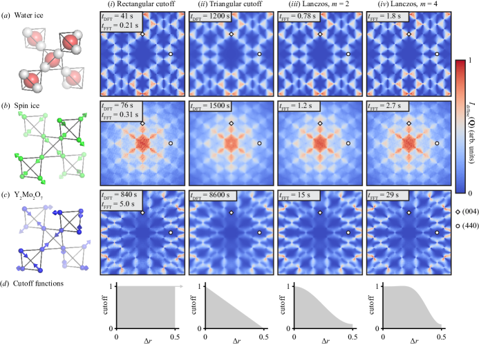
Figure 1: Diffuse-scattering calculations and real-space cutoff functions for different disorder models and methods of calculation. Rows (a)–(c) show results for three disorder models based on “ice rules”: (a) water ice (occupational disorder), (b) spin ice (magnetic disorder), and (c) Y₂Mo₂O₇ (displacive disorder). Row (d) shows the cutoff function defined in Eq. (11), where $\Delta r$ is the separation between atom pairs parallel to a crystal axis. For each row, columns show the calculated diffuse-scattering intensity $I_{\mathrm{diffuse}}(\mathbf{Q})$ obtained using different methods, and the corresponding cutoff function. Column (i) shows calculated intensities at the supercell Bragg positions obtained using Eqs. (29), (42), and (39) for rows (a)–(c), respectively. The calculated intensities shown in (a)i–(c)i contain noise and are not smooth functions of $\mathbf{Q}$, because the flat cutoff function shown in (d)i does not suppress long-range correlations that add to the noise. Column (ii) shows results for the method of sub-boxes Butler_1992 discussed in section V.1. The calculated intensities in (a)ii–(c)ii have low noise and are smooth functions of $\mathbf{Q}$, because the triangular cutoff function shown in (d)ii suppresses long-range correlations. Columns (iii) and (iv) show results for the Lanczos resampling approach discussed in section V.2 with $m=2$ and $m=4$, respectively, where $m$ is defined in Eq. (46). The Lanczos approach is an alternative to the method of sub-boxes. The calculated intensities in (a)iii–(c)iii and (a)iv–(c)iv again have reduced noise and are smooth functions of $\mathbf{Q}$, because the Lanczos cutoff functions shown in (d)iii and (d)iv suppresses long-range correlations by an amount determined by the parameter $m$. For each calculation of the diffuse-scattering intensity, the CPU time required for a calculation using the discrete Fourier transform $t_{\mathrm{DFT}}$ and/or the fast Fourier transform $t_{\mathrm{FFT}}$ is labelled. The FFT (+ optional Lanczos resampling) method produces accurate results and reduces the CPU time by between two and three orders of magnitude compared to the discrete Fourier transform (+ optional sub-boxes) method.

Figure 1(a)i–(c)i shows water-ice, spin-ice, and orbital-ice scattering calculations, respectively. The results for water ice and spin ice are in good agreement with published calculations Wehinger_2014 ; Fennell_2009 . Calculations using the discrete Fourier transform and the FFT gave identical results, as required. Crucially, however, the FFT-based calculations are much faster; e.g., the CPU time required for the FFT-based calculation of the water-ice scattering was $0.21$ s compared to $41$ s for the discrete-Fourier-transform calculation—an improvement of two orders of magnitude. Moreover, although 55 FFTs were required for the fifth-order approximation in the orbital-ice calculation, a reduction in CPU time of two orders of magnitude was still obtained. The largest error in any pixel for this fifth-order approximation was less than $0.7\%$, confirming that the Taylor expansion can be used for quantitative studies Butler_1993 .

To conclude this section, I discuss the performance of the FFT-based approach for scattering volumes and supercells that are much larger than those considered above. While Figure 1 shows a scattering plane, large scattering volumes can be calculated in a few minutes using the FFT; e.g., for the water-ice model, a cube in reciprocal space extending from $-12\leq h,k,l\leq 12$ and containing $\sim$$7\times 10^{6}$ supercell Bragg positions was calculated in $58$ s. Moreover, the $n_{1}n_{2}n_{3}\log_{2}(n_{1}n_{2}n_{3})$ scaling of the FFT means that larger supercells yield greater improvements in speed compared to the discrete Fourier transform; e.g., an FFT-based calculation for the spin-ice model using $40\times 40\times 40$ supercells, but otherwise equivalent to that shown in figure 1(b)i, was faster than the corresponding discrete-Fourier-transform calculation by a factor of approximately $1400$.

V Noise reduction

V.1 Method of sub-boxes

The scattering patterns shown in figure 1(a)i–(c)i, while of good quality, are affected by two problems. First, because the diffuse scattering has been calculated only at supercell Bragg positions, it is not a smooth function of wavevector. Second, the calculations are visibly affected by high-frequency noise (“speckle”), even though the results shown have been averaged over 100 independent supercells to reduce noise. As discussed in section I, this noise occurs because the calculation can be dominated by the many essentially-uncorrelated atom pairs that are large distances apart.

A proven approach to address these problems is to divide the supercell into a set of smaller overlapping regions, called “sub-boxes” or “lots” Butler_1992 ; Proffen_1997 . Each sub-box has open boundary conditions, and contains $n_{\mathrm{sb}}$ unit cells parallel to each crystal axis ($n_{\mathrm{sb}}^{3}$ unit cells in total). The value of $n_{\mathrm{sb}}$ should exceed the correlation length of the local modulations that generate the diffuse scattering, but be smaller than or equal to $n_{\alpha}/2$, to avoid contributions from periodic images of the supercell. The intensity for each sub-box is calculated separately using the discrete Fourier transform, and the results averaged to estimate $I(\mathbf{Q)}$. In the original algorithm, sub-boxes were distributed at random within the supercell, and the number of sub-boxes chosen so that each atom was included at least once Butler_1992 . However, this random-sampling approach has the disadvantage that a different answer is obtained each time the calculation is run. A recent algorithm addressed this problem by using every lattice point in the supercell as the origin of a sub-box, while avoiding unnecessary repetition of phase-factor calculations Paddison_2013b . I used this algorithm to perform scattering calculations for the example models discussed in section IV, using a sub-box length $n_{\mathrm{sb}}=5$ unit cells.

Figure 1(a)ii–(c)ii shows example scattering calculations using the method of sub-boxes. The use of open boundary conditions for each sub-box means that the calculation is not restricted to the Bragg positions of the supercell. Moreover, the calculation is essentially free of visible noise. There are two potential reasons for this. First, it is possible in general to choose $n_{\mathrm{sb}}<n_{\alpha}/2$, which excludes longer-range correlations from the calculation Butler_1992 . However, since I take $n_{\mathrm{sb}}=n_{\alpha}/2$, this reason does not apply in the present example. In fact, the method of sub-boxes is effective here because each sub-box has open boundary conditions, as I now discuss. I first recall that, for a periodic supercell, the number of distinct pairs of lattice points separated by $n_{\alpha}\Delta r_{\alpha}$ unit cells (parallel to crystal axis $\alpha$) is equal to $n_{\alpha}$; the cutoff function in Eq. (11) is therefore a rectangular function, as shown in figure 1(d)i. In contrast, if the supercell has open boundary conditions, then the number of distinct pairs of lattice points separated by $n_{\alpha}\Delta r_{\alpha}$ unit cells is equal to $n_{\alpha}(1-\Delta r_{\alpha})$. Consequently, the cutoff function for an open supercell is a triangular function that is equal to unity at $\Delta r_{\alpha}=0$ and zero at $\Delta r_{\alpha}=\pm 1$. Hence, in the method of sub-boxes, the cutoff function is also triangular and decays to zero at $\Delta r_{\alpha}=\pm n_{\mathrm{sb}}/n_{\alpha}$, as shown in figure 1(d)ii. This is the main result of this section. It explains how the method of sub-boxes reduces noise, because as the separation of atom pairs increases, their pair correlations are suppressed in the scattering calculation.

The analysis above also reveals two limitations of the method of sub-boxes. First, it is very much slower than the FFT-based approach. Indeed, it is also much slower than the discrete Fourier transform used to calculate $I(\mathbf{G})$ (figure 1(a)i–(c)i): this is mainly because the $401\times 401$ grid of wavevectors samples reciprocal space at finer intervals than the Nyquist rate defined by the spacing of the supercell Bragg positions, and hence calculates redundant information. Second, its effectiveness at reducing noise has the trade-off that the scattering is artificially blurred. Although this blurring can be reduced by increasing $n_{\mathrm{sb}}$, it is never entirely absent, because the triangular cutoff function is never flat. This limitation may be significant if accurate estimates of the correlation length are required.

V.2 Lanczos resampling

I now develop an approach that addresses the limitations of the method of sub-boxes, while maintaining its noise-reduction properties. Whereas the method of sub-boxes works directly in real space, I will show that its effects can be replicated efficiently by applying a resampling filter in reciprocal space.

I first recall that $I(\mathbf{Q})$ can, in principle, be calculated at any wavevector $\mathbf{Q}$ given only its samples at the supercell Bragg positions $\{\mathbf{G}\}$, by applying the Whittaker-Shannon interpolation formulae, Eqs. (12) and (13). Consequently, $I(\mathbf{G})$ can be calculated using the FFT and then resampled to obtain $I(\mathbf{Q})$ on a fine grid. An apparent problem with this resampling approach is that Eq. (12) requires summation over an infinite number of supercell Bragg positions to reproduce the discontinuity in the rectangular cutoff function at $\Delta r_{\alpha}=\pm r_{\mathrm{cut}}$. If the infinite summation is replaced by a finite summation, then large truncation artifacts (Fourier ripples) are introduced in the cutoff function, which do not vanish even as the number of summed terms becomes very large; this undesirable effect is known as the Gibbs phenomenon Gibbs_1899 . However, the key result of section V.1—that the method of sub-boxes effectively applies a triangular cutoff function—suggests that a rectangular cutoff function is not necessary or even desirable for diffuse-scattering calculations. The triangular cutoff function, and other suitably-chosen continuous functions, can be approximated by using a finite summation in Eq. (12). Consequently, the scattering intensity can be approximated as

$$I(\mathbf{Q}) \approx\frac{\sum_{\mathbf{G}}I(\mathbf{G})W(\mathbf{Q}-\mathbf{G})}{\sum_{\mathbf{G}}W(\mathbf{Q}-\mathbf{G})},$$ (44)

where the weight function $W(\mathbf{Q}-\mathbf{G})$ is the Fourier transform of the cutoff function, and the summation runs over supercell Bragg positions in the vicinity of $\mathbf{Q}$. This is the basis for the technique called Lanczos resampling Lanczos_1956 ; Duchon_1979 , which I discuss below.

The effects of Lanczos resampling in real and reciprocal space can be derived in three steps Duchon_1979 . First, the desired form of the cutoff function is specified. Second, $W(\mathbf{Q}-\mathbf{G})$ is determined as the Fourier transform of this idealized cutoff function. Third, $W(\mathbf{Q}-\mathbf{G})$ is back-Fourier-transformed numerically to determine the actual cutoff function obtained for a finite summation range. Following Lanczos Lanczos_1956 , I consider an idealized cutoff function that is equal to unity for $|\Delta r_{\alpha}|<0.5(1-2/m)$ and decays linearly to zero over the range $0.5(1-2/m)\leq|\Delta r_{\alpha}|\leq 0.5$, where $m\geq 2$ is an integer Duchon_1979 . Hereafter, the nominal cutoff separation $r_{\mathrm{cut}}=0.5(1-1/m)$ is the separation at which the idealized cutoff function equals $0.5$. Since this cutoff function is the convolution of two rectangular functions, its Fourier transform is the product of two sinc functions, so that

$$W(\mathbf{Q}-\mathbf{G})=W_{\mathrm{sinc}}(\mathbf{Q}-\mathbf{G})\thinspace L(\mathbf{Q}-\mathbf{G}),$$ (45)

where $W_{\mathrm{sinc}}(\mathbf{Q}-\mathbf{G})$ is given by Eq. (13) with $r_{\mathrm{cut}}=0.5(1-1/m)$, and

$$L(\mathbf{Q}-\mathbf{G}) =\begin{cases}\prod_{\alpha}\textrm{sinc}\left[\pi(Q_{\alpha}-G_{\alpha})/m\right]&\textrm{if }|Q_{\alpha}-G_{\alpha}|<m,\\ 0&\textrm{otherwise}\end{cases}$$ (46)

is called the window function. Because Eq. (46) is set to zero outside the central lobe of its sinc function Duchon_1979 , the summation in Eq. (44) is only taken over the $(2m)^{3}$ values of $\mathbf{G}$ for which $[Q_{\alpha}]-m+1\leq G_{\alpha}\leq[Q_{\alpha}]+m$, where square brackets denote the floor function. This approach is called windowed-sinc filtering. It has been widely used for image filtering and digital-signal processing Getreuer_2011 ; Marschner_1994 . It was applied to diffuse-scattering calculations for the first time by the present author Paddison_2018 ; a more detailed analysis is given here.

Example scattering calculations using Lanczos resampling with $m=2$ are shown in figure 1(a)iii–(c)iii and calculations with $m=4$ are shown in figure 1(a)iv–(c)iv. In each case, $I(\mathbf{G})$ was calculated using the FFT, and $I(\mathbf{Q})$ was then estimated using Eqs. (13) and (44)–(46). The corresponding cutoff functions are shown in figure 1(d)iii and 1(d)iv. The idealized cutoff function for the $m=2$ case is a triangular function, and the actual cutoff function resembles a smoothed version of it. Consequently, the scattering calculated by Lanczos resampling with $m=2$ closely resembles the sub-box calculation. The Lanczos approach is, however, faster than the method of sub-boxes by approximately three orders of magnitude. This large improvement arises first from the use of the FFT, and second because the scattering is only calculated at the supercell Bragg positions before being resampled to the $401\times 401$ pixel grid. As the value of $m$ is increased, the cutoff function increasingly resembles the rectangular function; hence, by tuning the value of $m$, it is possible to trade off the level of noise that can be tolerated against the amount of blur that is introduced. In particular, choosing $m>2$ ensures that the cutoff function is essentially flat for small $\Delta r_{\alpha}$, so that correlations at near-neighbour distances can be accurately reflected in the scattering pattern.

I mention three possible modifications to the Lanczos resampling approach. First, if $I(\mathbf{Q})$ is calculated on a grid with axes parallel to the reciprocal-lattice vectors, Eqs. (45) and (46) can be calculated along each axis in sequence, which reduces the computational expense associated with resampling Getreuer_2011 . Second, whereas the equations above assume that the idealized cutoff function decays to zero at $\Delta r_{\alpha}=0.5$, it may be preferable to choose a cutoff function that decays to zero at $\Delta r_{\alpha}<0.5$ if further noise suppression is required. This corresponds to choosing $n_{\mathrm{sb}}<n_{\alpha}/2$ in the method of sub-boxes. In the Lanczos approach, an idealized cutoff function with $r_{\mathrm{cut}}=(1-1/m)/m^{\prime}$ that decays to zero at $|\Delta r_{\alpha}|=1/m^{\prime}$ can be obtained for integer $m^{\prime}>2$ by replacing $m$ with $mm^{\prime}/2$ in Eq. (46). Finally, it may sometimes be preferable to use a spherically-symmetric cutoff function. This can be achieved by replacing Eq. (13) with

$$W_{\mathrm{r}}(|\mathbf{Q}-\mathbf{G}|)=\frac{4\pi|\mathbf{r}_{\mathrm{c}}|^{3}}{n_{1}n_{2}n_{3}V}\left[\frac{\sin(|\mathbf{Q}||\mathbf{r}_{\mathrm{c}}|)}{(|\mathbf{Q}||\mathbf{r}_{\mathrm{c}}|)^{3}}-\frac{\cos(|\mathbf{Q}||\mathbf{r}_{\mathrm{c}}|)}{(|\mathbf{Q}||\mathbf{r}_{\mathrm{c}}|)^{2}}\right],$$ (47)

where $|\mathbf{r}_{\mathrm{c}}|=(1-1/m)|\mathbf{r}_{\mathrm{max}}|$, $|\mathbf{r}_{\mathrm{max}}|$ is the radius of the largest sphere that can be inscribed in the supercell, and $n_{1}n_{2}n_{3}V$ is the supercell volume Marschner_1994 .

VI Conclusions

The main result of this article is that diffuse-scattering calculations from atomistic models can be accelerated by at least two orders of magnitude by applying two fundamental properties of scattering patterns. The first is that the average lattice of a crystal has the periodicity of the crystallographic unit cell, even in the presence of disorder; this property allows the fast Fourier transform (FFT) algorithm to be used to calculate diffuse scattering, which has not previously been considered feasible Butler_1992 . The second is that the scattering intensity of a periodic supercell is determined at all wavevectors by its values at the Bragg positions of the supercell; this observation allows the scattering intensity to be determined on an arbitrarily fine wavevector grid without redundant calculations. These observations are by no means new: indeed, they date to the earliest work on structural disorder Borie_1971 and sampling theory in crystallography Sayre_1952 . Nevertheless, their importance for diffuse-scattering calculations has not previously been recognized.

The acceleration of diffuse-scattering calculations enabled by these results and the associated computer program Scatty [27] has important practical implications. Comparisons of model calculations with the large 3D datasets obtained by modern X-ray and neutron instruments would previously have required many hours, but can now be performed in a few minutes on a laptop. Moreover, it is now practical to fit models of the interactions between disorder variables (local displacements, occupancies, or magnetic moments) directly to 3D experimental datasets in a matter of hours; such fits would previously have required many weeks or months, which has proved prohibitive Welberry_1998 ; Welberry_2008 . It is also possible to parallelize the intensity calculations for many supercells, potentially leading to further reductions in computer time Gutmann_2010 . I therefore anticipate that these developments will make quantitative analysis of large diffuse-scattering datasets more practical, more quantitative, and more easily automated. I hope that, similar to the advent of 3D data analysis in conventional crystallography approximately 60 years ago, the prospect of 3D diffuse-scattering analysis identified previously Welberry_2008 will allow the diffuse-scattering approach to be applied to a much wider range of disordered crystalline materials than has yet been possible.

- (1) B. D. Butler, T. R. Welberry, J. Appl. Cryst. 25, 391 (1992).
- (2) D. A. Keen, J. Phys.: Condens. Matter 14, R819 (2002).
- (3) T. Fennell, P. P. Deen, A. R. Wildes, K. Schmalzl, D. Prabhakaran, A. T. Boothroyd, R. J. Aldus, D. F. McMorrow, S. T. Bramwell, Science 326, 415 (2009).
- (4) J. A. M. Paddison, J. R. Stewart, P. Manuel, P. Courtois, G. J. McIntyre, B. D. Rainford, A. L. Goodwin, Phys. Rev. Lett. 110, 267207 (2013).
- (5) G. Xu, Z. Zhong, H. Hiraka, G. Shirane, Phys. Rev. B 70, 174109 (2004).
- (6) M. Paściak, T. R. Welberry, J. Kulda, M. Kempa, J. Hlinka, Phys. Rev. B 85, 224109 (2012).
- (7) S. Shimomura, N. Wakabayashi, H. Kuwahara, Y. Tokura, Phys. Rev. Lett. 83, 4389 (1999).
- (8) S. J. L. Billinge, I. Levin, Science 316, 561 (2007).
- (9) D. A. Keen, A. L. Goodwin, Nature 521, 303 EP (2015).
- (10) A. R. Overy, A. B. Cairns, M. J. Cliffe, A. Simonov, M. G. Tucker, A. L. Goodwin, Nat. Commun. 7, 10445 EP (2016).
- (11) T. Weber, A. Simonov, Z. Kristallogr. 227, 238 (2012).
- (12) D. A. Keen, M. J. Gutmann, C. C. Wilson, J. Appl. Cryst. 39, 714 (2006).
- (13) F. Ye, Y. Liu, R. Whitfield, R. Osborn, S. Rosenkranz, J. Appl. Cryst. 51, 315 (2018).
- (14) P. Kraft, A. Bergamaschi, C. Broennimann, R. Dinapoli, E. F. Eikenberry, B. Henrich, I. Johnson, A. Mozzanica, C. M. Schlepütz, P. R. Willmott, B. Schmitt, J. Synchrotron Rad. 16, 368 (2009).
- (15) M. J. Gutmann, K. Refson, M. v Zimmermann, I. P. Swainson, A. Dabkowski, H. Dabkowska, J. Phys.: Condens. Matter 25, 315402 (2013).
- (16) T. R. Welberry, T. Proffen, M. Bown, Acta Cryst. A 54, 661 (1998).
- (17) T. R. Welberry, D. J. Goossens, Acta Cryst. A 64, 23 (2008).
- (18) T. Weber, H.-B. Bürgi, Acta Cryst. A 58, 526 (2002).
- (19) R. L. McGreevy, L. Pusztai, Mol. Simul. 1, 359 (1988).
- (20) M. G. Tucker, D. A. Keen, M. T. Dove, A. L. Goodwin, Q. Hui, J. Phys.: Condens. Matter 19, 335218 (2007).
- (21) J. A. M. Paddison, A. L. Goodwin, Phys. Rev. Lett. 108, 017204 (2012).
- (22) J. W. Cooley, J. W. Tukey, Math. Comput. 19, 297 (1965).
- (23) R. B. Neder, U. Wildgruber, Z. Kristallogr. 186, 209 (1989).
- (24) S. H. Rahman, Z. Kristallogr. 186, 116 (1989).
- (25) T. Proffen, R. B. Neder, J. Appl. Cryst. 30, 171 (1997).
- (26) M. J. Gutmann, J. Appl. Cryst. 43, 250 (2010).
- (27) The program Scatty can be downloaded from https://paddisongroup.wordpress.com/software.
- (28) T. Egami, S. J. L. Billinge, Underneath the Bragg Peaks: Structural Analysis of Complex Materials (Elsevier, Oxford, 2003), vol. 7 of Pergamon Materials Series, first edn.
- (29) A. L. Goodwin, M. G. Tucker, M. T. Dove, D. A. Keen, Phys. Rev. Lett. 93, 075502 (2004).
- (30) F. Frey, Z. Kristallogr. 212, 257 (1997).
- (31) E. Whittaker, P. Roy. Soc. Edinb. A 35, 181 (1915).
- (32) C. E. Shannon, Proc. IRE 37, 10 (1949).
- (33) D. Sayre, Acta Cryst. 5, 843 (1952).
- (34) R. Singleton, IEEE Trans. Audio and Electroacoustics 17, 93 (1969).
- (35) D. J. Goossens, A. P. Heerdegen, E. J. Chan, T. R. Welberry, Metal. Mater. Trans. A 42, 23 (2011).
- (36) T. M. Michels-Clark, Methods for quantitative local structure analysis of crystalline materials employing high performance computing, Ph.D. thesis, University of Tennessee–Knoxville (2014).
- (37) R. Withers, IUCrJ 2, 74 (2015).
- (38) B. Borie, C. J. Sparks, Jnr, Acta Cryst. A 27, 198 (1971).
- (39) M. Hayakawa, J. B. Cohen, Acta Cryst. A 31, 635 (1975).
- (40) G. L. Squires, Introduction to the Theory of Thermal Neutron Scattering (Cambridge University Press, Cambridge, 1978).
- (41) S. W. Lovesey, Theory of Neutron Scattering from Condensed Matter: Polarization Effects and Magnetic Scattering, vol. 2 (Oxford University Press, Oxford, 1987).
- (42) P. H. Conlon, Aspects of frustrated magnetism, Ph.D. thesis, University of Oxford (2010).
- (43) S. T. Bramwell, M. J. Gingras, Science 294, 1495 (2001).
- (44) L. Pauling, J. Am. Chem. Soc. 57, 2680 (1935).
- (45) W. F. Giauque, J. W. Stout, J. Am. Chem. Soc. 58, 1144 (1936).
- (46) A. P. Ramirez, A. Hayashi, R. J. Cava, R. Siddharthan, B. S. Shastry, Nature 399, 333 (1999).
- (47) J. S. Gardner, B. D. Gaulin, S.-H. Lee, C. Broholm, N. P. Raju, J. E. Greedan, Phys. Rev. Lett. 83, 211 (1999).
- (48) P. M. M. Thygesen, J. A. M. Paddison, R. Zhang, K. A. Beyer, K. W. Chapman, H. Y. Playford, M. G. Tucker, D. A. Keen, M. A. Hayward, A. L. Goodwin, Phys. Rev. Lett. 118, 067201 (2017).
- (49) B. Wehinger, D. Chernyshov, M. Krisch, S. Bulat, V. Ezhov, A. Bosak, J. Phys.: Condens. Matter 26, 265401 (2014).
- (50) B. D. Butler, T. R. Welberry, Acta Cryst. A 49, 736 (1993).
- (51) J. A. M. Paddison, J. R. Stewart, A. L. Goodwin, J. Phys.: Condens. Matter 25, 454220 (2013).
- (52) J. W. Gibbs, Nature 59, 606 (1899).
- (53) C. Lanczos, Applied Analysis (Prentice-Hall, Englewood Cliffs, New Jersey, 1956).
- (54) C. E. Duchon, J. Appl. Meteorol. 18, 1016 (1979).
- (55) P. Getreuer, IPOL Image Proc. On Line 1, 238 (2011).
- (56) S. R. Marschner, R. J. Lobb, Proceedings of the Conference on Visualization ’94, VIS ’94 (IEEE Computer Society Press, Los Alamitos, CA, USA, 1994), pp. 100–107.
- (57) J. A. M. Paddison, M. J. Gutmann, J. R. Stewart, M. G. Tucker, M. T. Dove, D. A. Keen, A. L. Goodwin, Phys. Rev. B 97, 014429 (2018).