Dynamical Optimal Transport on Discrete Surfaces

Abstract.

We propose a technique for interpolating between probability distributions on discrete surfaces, based on the theory of optimal transport. Unlike previous attempts that use linear programming, our method is based on a dynamical formulation of quadratic optimal transport proposed for flat domains by Benamou and Brenier [2000], adapted to discrete surfaces. Our structure-preserving construction yields a Riemannian metric on the (finite-dimensional) space of probability distributions on a discrete surface, which translates the so-called Otto calculus to discrete language. From a practical perspective, our technique provides a smooth interpolation between distributions on discrete surfaces with less diffusion than state-of-the-art algorithms involving entropic regularization. Beyond interpolation, we show how our discrete notion of optimal transport extends to other tasks, such as distribution-valued Dirichlet problems and time integration of gradient flows.

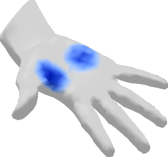
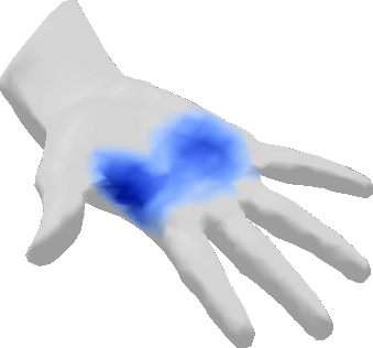
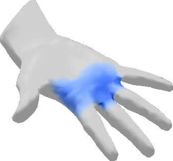
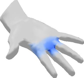
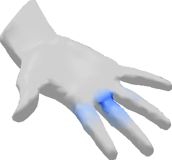
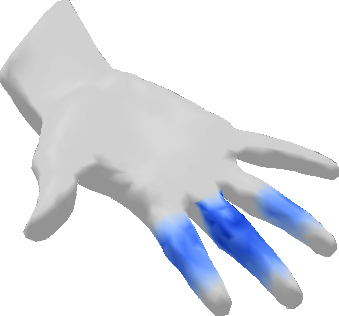
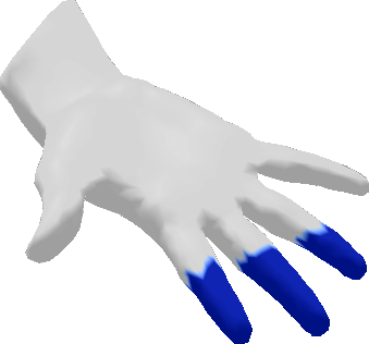
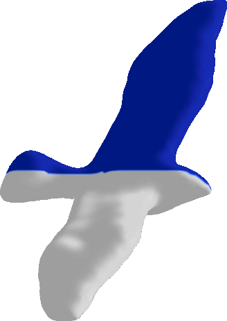
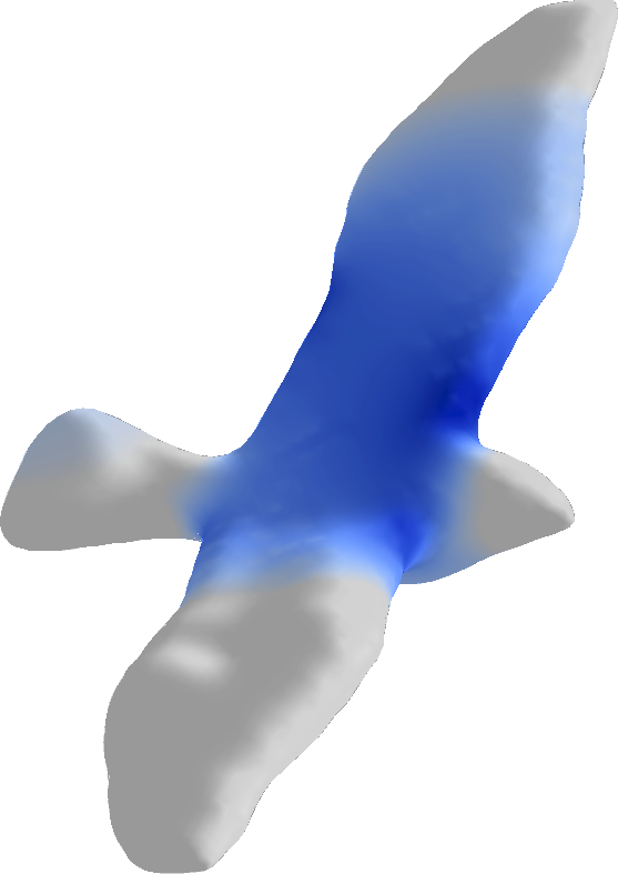
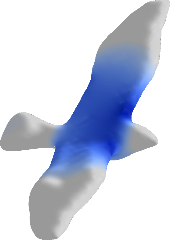
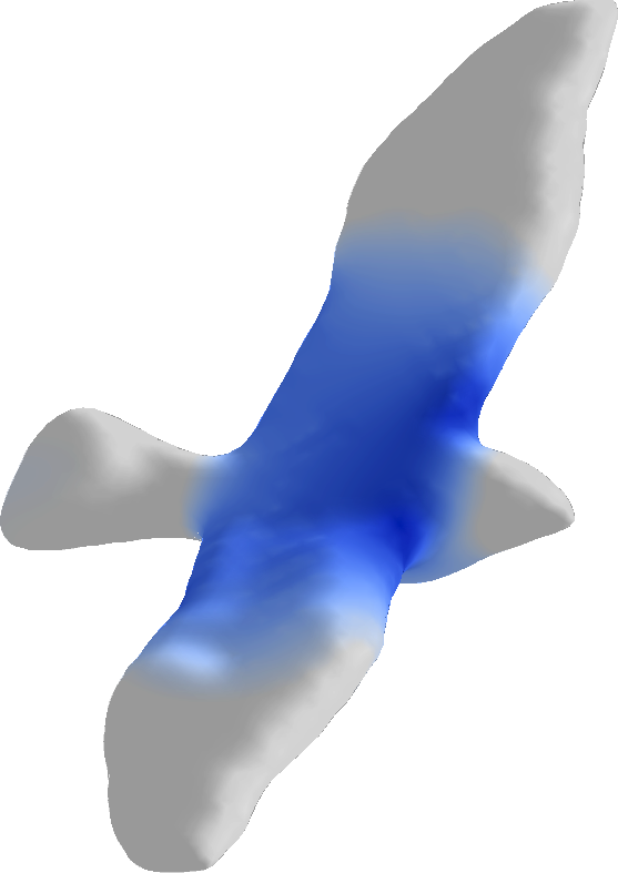
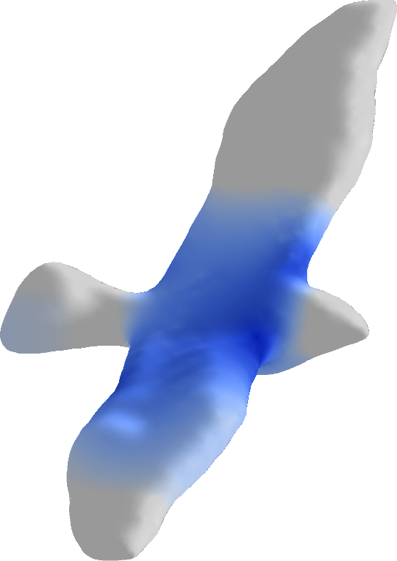
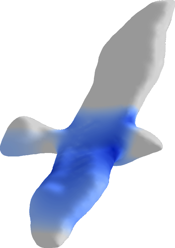
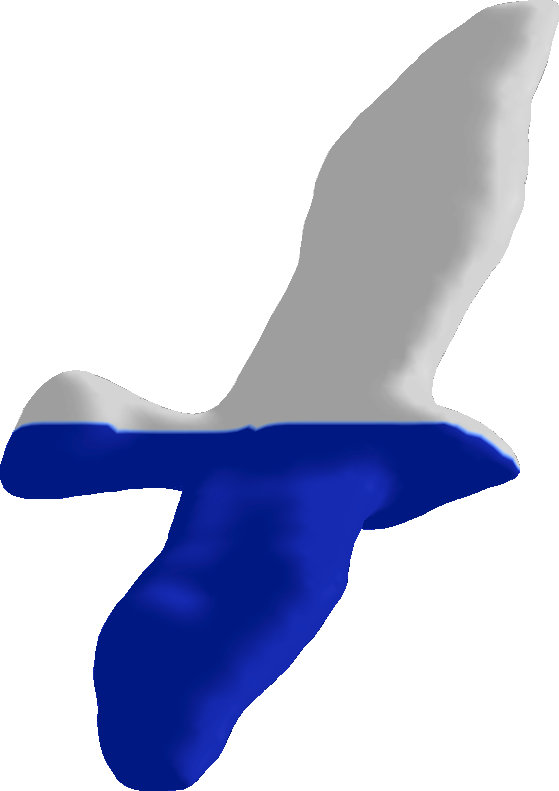
Figure 1. Given two probability distributions over a discrete surface (left and right), our algorithm generates an interpolation that takes the geometric structure of the surface into account.

1. Introduction

Probability distributions are key objects in geometry processing that can encode a variety of quantities, including uncertain feature locations on a surface, color histograms, and physical measurements like the density of a fluid. A central problem related to distributions is that of interpolation: Given two probability distributions over a fixed domain, how can one transition smoothly from the first to the second?

Optimal transport gives one potential solution. This theory lifts the geometric structure of a surface to a Riemannian structure on the space of probability distributions over the surface, the latter being endowed with the so-called Wasserstein metric; the set of distributions equipped with this metric is sometimes called Wasserstein space. To interpolate between two probability distributions, one computes a geodesic in Wasserstein space between the two. This definition is sometimes referred to as McCann’s displacement interpolation [1997], applied to graphics e.g. in [Bonneel et al., 2011].

Even though optimal transport theory is now well-understood [Villani, 2003, 2008; Santambrogio, 2015], the interpolation problem remains challenging numerically. Related problems, like the computation of Wasserstein distances or barycenters in Wasserstein space, can be tackled by fast and scalable algorithms like entropic regularization or semi-discrete methods, developed only a few years ago. Most of these methods, however, fail to reproduce the Riemannian structure of Wasserstein space and/or are prone to diffusion: The interpolation between two peaked probability distributions is more diffuse in the midpoint than optimal transport theory suggests. This drawback can inhibit application of transport in computer graphics practice, in which blurry interpolants are often undesirable.

As an alternative, we define a Riemannian structure on the space of probability distributions over a discrete surface, designed to mimic that of the Wasserstein distance between distributions over a smooth manifold. Our construction is inspired by the Benamou–Brenier formula [2000], previously discretized only on flat grids without structure preservation. This Riemannian structure automatically defines geodesics and distances between probability distributions. In particular, the geodesic problem can be recast as a convex problem and be tackled by iterative methods phrased using local operators familiar in geometry processing and finite elements (gradients, divergence and Laplacian on the surface). Our method does not require precomputation of pairwise distances between points on the surface.

Compared to other methods, our interpolation can be rephrased as a geodesic problem and numerically exhibits less diffusion when interpolating between peaked distributions. In cases where the sharpness captured by our method and predicted by optimal transport theory is undesirable visually, we provide a quadratic regularizer that controllably reduces congestion of the computed interpolant; unlike entropically-regularized transport, however, our optimization problem does not degenerate or become harder to solve when the regularization term vanishes. Although the computation of interpolants remains quite slow for meshes with more than a few thousand vertices and improving the scalability of numerical routines used to optimize our convex objective remains a challenging task for future work, we demonstrate application to tasks derived from transport, e.g. computation of harmonic mappings into Wasserstein space and integration of gradient flows.

In addition to our algorithmic contributions, we regard our work as a key theoretical step toward making optimal transport compatible with the language of discrete differential geometry (DDG). Our Riemannian metric induces a true geodesic distance—with a triangle inequality—on the space of distributions over a triangulated surface expressed using one value per vertex. Inspired by an analogous construction on graphs [Maas, 2011], we leverage a non-obvious observation that a strong contender for structure-preserving discrete transport on meshes actually involves a real-valued external time variable, rather than discretizing transport as a linear program as in most previous work. The resulting geodesic problem naturally preserves convexity and other key properties from the theoretical case while suggesting an effective computational technique.

2. Related work

2.1. Linear programming and regularization

Landmark work by Kantorovich [1942] showed that optimal transport can be phrased as a linear programming problem. If both probability distributions have finite support, we end up with a finite-dimensional linear program solvable using standard convex programming techniques. A variety of solvers has been designed to tackle this linear program, which exploit the particular structure of the objective functional [Edmonds and Karp, 1972; Klein, 1967; Orlin, 1997]. These methods, however, usually require as input the pairwise distance matrix, a dense matrix that scales quadratically in the size of the support and is difficult to evaluate if the points are on a curved space.

A landmark paper by Cuturi [2013] reinvigorated interest in numerical transport by proposing adding an entropic regularizer to the problem, leading to the efficient Sinkhorn (or matrix rebalancing) algorithm. This algorithm, which involves iteratively rescaling the rows and columns of a kernel in the cost matrix, is highly parallelizable and well-suited to GPU architectures. When the cost matrix involves squared geodesic distances along a discrete surface, Solomon et al. [2015] showed that Sinkhorn iterations can be written in terms of heat diffusion operators, eliminating the need to store the cost matrix explicitly. While they are efficient, these entropically-regularized techniques suffer from diffusion, making them less relevant to problems in which measures are sharp or peaked. They also do not define true distances on the space of distributions over mesh vertices.

When the transport cost is equal to geodesic distance, i.e. the $1$-Wasserstein distance, optimal transport is equivalent to the Beckmann problem [Santambrogio, 2015, Chapter 4], for which specific and efficient algorithms can be designed [Solomon et al., 2014; Li et al., 2018]. These methods cannot be applied to the quadratic Wasserstein distance, which is needed to make transport-based interpolation nontrivial, namely to recover McCann’s displacement interpolation [1997]. In particular, the optimal transport problem defining the $1$-Wasserstein distance does not come with a time dependency allowing to define a smooth interpolation and suffers from non-uniqueness coming from the lack of strict convexity.

2.2. Semi-discrete optimal transport

When one of the distributions has a density w.r.t. Lebesgue while the other one is discrete, the transport problem can be reduced to a finite-dimensional convex problem whose number of unknowns scales with the cardinality of the support of the discrete distribution. Leveraging tools from computational geometry, this semi-discrete problem can be solved efficiently up to fairly large scale when the cost is Euclidean [Aurenhammer et al., 1998; Mérigot, 2011; De Goes et al., 2012; Lévy, 2015; Kitagawa et al., 2016].

Semi-discrete transport has been used to tackle problems for which the precise structure of the optimal transportation map is relevant, as in fluid dynamics [de Goes et al., 2015b; Mérigot and Mirebeau, 2016; Gallouët and Mérigot, 2017]. It also has been used for approximating barycenters in the stochastic case [Claici et al., 2018] and as a measure of proximity for shape reconstruction [de Goes et al., 2011; Digne et al., 2014]. Extensions of semi-discrete transport to curved spaces can be found in [de Goes et al., 2014; Mérigot et al., 2018]. Although they can be fast and give explicit transport maps, these methods are not suited for the application we have in mind: They rely on the computation of transport maps between two probability distributions that are not of the same nature (one is discrete, the other has a density) and hence cannot be used to implement a distance or interpolation cleanly.

2.3. Fluid dynamic formulations

By switching from Lagrangian to Eulerian descriptions of transport, Benamou and Brenier [2000] proved that optimal transport could be rephrased using fluid dynamics: Instead of computing a coupling, they show that transport with quadratic costs is equivalent to finding a time-varying sequence of distributions smoothly interpolating between the two measures. The problem that they obtain is convex and solved via the Alternating Direction Method of Multipliers (ADMM) [Boyd et al., 2011]. Proof of the convergence of ADMM in the infinite-dimensional setting (i.e. when neither time nor the geometric domain is discretized) is provided in [Guittet, 2003; Hug et al., 2015]. Papadakis et al. [2014] reread the ADMM iterations as a proximal splitting scheme and show how one can build different algorithms to solve the convex problem. This fluid dynamic formulation also appears in mean field games [Benamou and Carlier, 2015].

In all of the above work, however, the authors work in a flat space and use finite difference discretizations of the densities and velocity fields. Hence their work does not contain a clear indication about how to handle the problem on a discrete curved space, and theoretical properties of their models after discretization remain unverified.

The algorithm for approximating 1-Wasserstein distances presented by Solomon et al. [2014] achieves some of the objectives mentioned above. Their vector field formulation is in some sense dynamical, and their distance satisfies properties like the triangle inequality after discretization. As mentioned above, however, their optimization problem lacks strict convexity and is not suitable for interpolation.

2.4. Dynamical transport on graphs and meshes

Maas [2011] defines a Wasserstein distance between probability distributions over the vertices of a graph. The (finite-dimensional) space of distributions in this case inherits a Riemannian metric with some structure preserved from the infinite-dimensional definition; for instance, the gradient flow of entropy corresponds to a notion of heat flow along the graph. A similar structure is proposed by Chow et al. [2016], but they recover a different heat flow. Erbar et al. [2017] propose a numerical algorithm for approximating the discrete Wasserstein distance introduced by Maas, but the distributions they produce have a tendency to diffuse along the graph. This flaw is not related to their numerical method but rather comes from the very definition of their optimal transport distance. It is also not obvious what is the best way to adapt their construction to discrete surfaces rather than graphs.

2.5. Interpolation and geodesics

Optimal transport is not the only way to interpolate between probability distributions; for instance, Azencot et al. [2016] use a time-independent velocity field to advect functions and match them. Their method, however, cannot be understood as a geodesic curve in the space of distributions. In another direction, Heeren et al. [2012] have provided an efficient way to discretize in time geodesics in a high-dimensional space of thin shells. Their formulation is not well-suited for optimal transport where direct discretization of the Benamou–Brenier formula is possible. Finally, methods like [Panozzo et al., 2013] provide a means of averaging points on discrete surfaces, although it is not clear how to extend them to the more general distribution case.

3. Optimal transport on a discrete surface

$t=0$	$t=\nicefrac{{1}}{{4}}$	$t=\nicefrac{{1}}{{2}}$	$t=\nicefrac{{3}}{{4}}$	$t=1$

Figure 2. Top row: Interpolation of probability distributions. The left and right distributions are data and the middle ones are the output of our algorithm. Bottom row: Display of the momentum $\mathbf{m}=\mu\mathbf{v}$, where $\mathbf{v}$ is a time-dependent velocity-field advecting the left distrbution on the right one. We have used the regularization described in Subsection 5.4 with $\alpha=0.1$.

3.1. Optimal transport on manifolds

$t=0$	$t=\nicefrac{{1}}{{3}}$	$t=\nicefrac{{2}}{{3}}$	$t=1$

Figure 3. Top row: schematic view of the static formulation of optimal transport (1). The initial distribution $\bar{\mu}^{0}$ is on the left, and the final distribution $\bar{\mu}^{1}$ is on the right. The quantity $\mathrm{d}\pi(x,y)$ represents the amount of mass that is transported from $x$ to $y$. The coupling $\pi$ is chosen in such a way that the total cost is minimal. Bottom row: dynamical formulation between the same distributions (computed with the algorithm in Section 4). To go from the top to the bottom row, once one has the optimal $\pi$, a proportion $\mathrm{d}\pi(x,y)$ of particles follows the geodesic (in this case a straight line) between $x$ and $y$ with constant speed. The macroscopic result of all these motions is a time-varying sequence of distributions, displayed in blue.

We begin by introducing briefly optimal transport theory on a smooth space. Let $\mathcal{M}$ be a connected and compact Riemannian manifold with metric $\langle\ ,\ \rangle$ and induced norm $\|\ \|$; define $d:\mathcal{M}\times\mathcal{M}\to\mathbb{R}_{+}$ to be geodesic distance.

Denote by $\mathcal{P}(\mathcal{M})$ the space of probability measures on $\mathcal{M}$. This space is endowed with the quadratic Wasserstein distance from optimal transport: If $\bar{\mu}^{0},\bar{\mu}^{1}\in\mathcal{P}(\mathcal{M})$, then the distance $W_{2}(\bar{\mu}^{0},\bar{\mu}^{1})$ between them is defined as

(1) $$W_{2}^{2}(\bar{\mu}^{0},\bar{\mu}^{1}):=\min_{\pi}\iint_{\mathcal{M}\times\mathcal{M}}\frac{1}{2}d(x,y)^{2}\mathrm{d}\pi(x,y),$$

where the minimum is taken over all probability measures $\pi$ on the product space $\mathcal{M}\times\mathcal{M}$ whose first (resp. second) marginal is $\bar{\mu}^{0}$ (resp. $\bar{\mu}^{1}$).

The problem (1) can be interpreted as follows: $\mathrm{d}\pi(x,y)$ denotes the quantity of particles located at $x$ that are sent to $y$, and the cost for such a displacement is $d(x,y)^{2}$. The constraint on the marginals enforces that $\pi$ describes a way of moving the distribution of mass $\bar{\mu}^{0}$ onto $\bar{\mu}^{1}$. Thus, the variational problem (1) reads: Find the cheapest way $\pi$ to send $\bar{\mu}^{0}$ onto $\bar{\mu}^{1}$, and the result (i.e. the minimal cost) is defined as the squared Wasserstein distance between $\bar{\mu}^{0}$ and $\bar{\mu}^{1}$. In some generic cases [Brenier, 1991; Gangbo and McCann, 1996], the optimal $\pi$ is located on the graph of a map $T:\mathcal{M}\to\mathcal{M}$, which means that a particle $x\in\mathcal{M}$ is sent onto a unique location $y=T(x)\in\mathcal{M}$.

The space $(\mathcal{P}(\mathcal{M}),W_{2})$ is a complete metric space [Santambrogio, 2015; Villani, 2003], and—at least formally—it has the structure of an (infinite-dimensional) Riemannian manifold. Revealing this manifold structure requires some manipulation and rephrasing of the original problem (1), detailed below.

As first noticed by Benamou and Brenier [2000], the Wasserstein distance between $\bar{\mu}^{0}$ and $\bar{\mu}^{1}$ can be obtained by solving an alternative, physically-motivated optimization problem:

(2) $$W_{2}^{2}(\bar{\mu}^{0},\bar{\mu}^{1})=\begin{cases}\min_{\mu,\mathbf{v}}&\int_{0}^{1}\int_{\mathcal{M}}\frac{1}{2}\|\mathbf{v}^{t}\|^{2}\mathrm{d}\mu^{t}\mathrm{d}t\\ \text{s.t. }&\mu^{0}=\bar{\mu}^{0},\ \mu^{1}=\bar{\mu}^{1},\\ &\partial_{t}\mu+\nabla\cdot(\mu\mathbf{v})=0.\end{cases}$$

As we will have to deal with functions and vectors depending both on time and space, here and moving forward we adopt the following convention: Upper indices denote time, and lower indices denote space. Moreover, $t\in[0,1]$ will denote an instant in time, and $f$ will later denote a generic triangle ($f$ for face) in a triangulation. In (2), the minimum is taken over all curves $\mu:[0,1]\to\mathcal{P}(\mathcal{M})$ and all time-dependent velocity fields $\mathbf{v}:[0,1]\times\mathcal{M}\to T\mathcal{M}$ such that the continuity equation $\partial_{t}\mu+\nabla\cdot(\mu\mathbf{v})=0$ is satisfied in the sense of distributions. The optimal curve $\mu$ is known as McCann’s displacement interpolation [1997].

The physical interpretation of this problem is as follows. Imagine probability distributions as distributions of mass, e.g. the density of a fluid. The curve $\mu$ represents an assembly of particles in motion, distributed as $\bar{\mu}^{0}$ at $t=0$ and $\bar{\mu}^{1}$ at $t=1$. At time $t$, a particle located at $x\in\mathcal{M}$ moves with velocity $\mathbf{v}^{t}_{x}$. The continuity equation $\partial_{t}\mu+\nabla\cdot(\mu\mathbf{v})=0$ simply expresses the conservation of mass. For a given time $t$, the cost $\int_{\mathcal{M}}\frac{1}{2}\|\mathbf{v}^{t}\|^{2}\mathrm{d}\mu^{t}$ is the total kinetic energy of all the particles. Hence, the cost minimized in (2), i.e. the integral w.r.t. time of the kinetic energy, is the action of the curve. As there is no congestion cost—that is, the particles do not interact with each other—(2) is the least-action principle for a pressureless gas.

Formulation (1) is static, since it directly determines the target for each particle at $t=1$ given the arrangement at $t=0$. On the other hand, (2) is dynamical, recovering a curve in $\mathcal{P}(\mathcal{M})$ interpolating smoothly between $\bar{\mu}^{0}$ and $\bar{\mu}^{1}$. To convert from the static to the dynamical formulation, one takes an optimal transport plan $\pi$ from (1) and an assembly of particles distributed according to $\bar{\mu}^{0}$. If a particle located at $x\in\mathcal{M}$ at time $t=0$ and is supposed, according to $\pi$, to be sent to $y\in\mathcal{M}$, then this particle follows a constant-speed geodesic along $\mathcal{M}$ from $x$ to $y$. The optimal curve $\mu$ in (2) is exactly the resulting macroscopic motion of all the particles, illustrated in Figure 3.

Calling $\mathbf{m}=\mu\mathbf{v}$ the momentum and using the change of variables $(\mu,\mathbf{v})\leftrightarrow(\mu,\mathbf{m})$, problem (2) becomes convex, because the mapping $(\mu,\mathbf{v})\to\nicefrac{{1}}{{2}}\|\mathbf{v}\|^{2}\mu$ is not jointly convex while $(\mu,\mathbf{m})\to\nicefrac{{1}}{{2}}\|\mathbf{m}\|^{2}/\mu$ is. Its dual reads

(3) $$W_{2}^{2}(\bar{\mu}^{0},\bar{\mu}^{1})=\begin{cases}\max_{\varphi}&\int_{\mathcal{M}}\varphi^{1}\mathrm{d}\bar{\mu}^{1}-\int_{\mathcal{M}}\varphi^{0}\mathrm{d}\bar{\mu}^{0}\\ \text{s.t. }&\partial_{t}\varphi+\frac{1}{2}\|\nabla\varphi\|^{2}\leqslant 0\text{ on }[0,1]\times\mathcal{M},\end{cases}$$

where the maximization is performed over real-valued functions $\varphi:[0,1]\times\mathcal{M}\to\mathbb{R}$ [Villani, 2008; Santambrogio, 2015]. The relation $\mathbf{v}=\nabla\varphi$ holds whenever $\mathbf{v}$ (resp. $\varphi$) is a minimizer (resp. maximizer) of the primal (resp. dual) problem. In particular, in (2), we can restrict ourselves to the set of $\mathbf{v}$ such that $\mathbf{v}^{t}=\nabla\varphi^{t}$ for every $t\in[0,1]$.

Equation (2) defines a formal Riemannian structure on $\mathcal{P}(\mathcal{M})$ [Otto, 2001]. Given $\mu\in\mathcal{P}(\mathcal{M})$ with a density bounded from below by a strictly positive constant, the tangent space $T_{\mu}\mathcal{P}(\mathcal{M})$ is identified as the set of functions $\delta\mu:\mathcal{M}\to\mathbb{R}$ with $0$-mean: $\delta\mu$ is the partial derivative w.r.t. time of a curve whose value at time $0$ is $\mu$. If $\delta\mu\in T_{\mu}\mathcal{P}(\mathcal{M})$, we can compute $\varphi:\mathcal{M}\to\mathbb{R}$ the solution (unique up to translation by constants) of the elliptic equation

(4) $$\nabla\cdot(\mu\nabla\varphi)=-\delta\mu.$$

Then, the norm of $\delta\mu$ is defined as

(5) $$\|\delta\mu\|^{2}_{T_{\mu}\mathcal{P}(\mathcal{M})}:=\frac{1}{2}\int_{\mathcal{M}}\|\nabla\varphi\|^{2}\mathrm{d}\mu.$$

Endowed with this scalar product obtained from the polarization identity $\langle x,y\rangle=\frac{1}{4}(\|x+y\|^{2}-\|x-y\|^{2})$, one can check, and the derivation appears in the supplemental material, that the Wasserstein distance $W_{2}$ can be interpreted as the geodesic distance induced by (4) and (5). This is precisely the content of the Benamou–Brenier formula (2).

One needs to assume $\mu\geqslant c>0$ on $\mathcal{M}$ for the elliptic equation (4) to be well-posed. Nevertheless, one can still give a meaning to this Riemannian structure using tools from analysis in metric spaces [Ambrosio et al., 2008].

3.2. Discrete surfaces

The previous subsection contains only well-understood results. Let us now start our contribution: to mimic these definitions and properties when the manifold is replaced by a triangulated surface.

Instead of a smooth manifold $\mathcal{M}$, we consider the case where we only have access to a triangulated surface $S=(V,E,T)$, which consists of a set $V\subset\mathbb{R}^{3}$ of vertices, a set $E\subseteq V\times V$ of edges linking vertices, and a set $T\subseteq V\times V\times V$ of triangles containing exactly $3$ vertices linked by $3$ edges. For a given face $f\in T$, we denote by $V_{f}\subset V$ the set of vertices $v$ such that $v\in f$; for a given vertex $v\in V$, we denote by $T_{v}\subset T$ the set of faces $f$ such that $v\in f$. The area of a triangle $f\in T$ is denoted by $|f|$. Each vertex $v$ is associated to a barycentric dual cell (see Figure 4) whose area, equal to $\frac{1}{3}\sum_{f\in T_{v}}|f|$, is denoted by $|v|$.

Following standard constructions from first-order finite elements (FEM), a scalar function on $\mathcal{M}$ will be seen as having one value per vertex, i.e. belonging to $\mathbb{R}^{|V|}$. A distribution $\mu\in\mathcal{M}$ will be also discretized by one value per vertex representing the density w.r.t. the volume measure. In other words, the volume of the dual cell centered at $v\in V$, measured with $\mu$, is $|v|\mu_{v}$. We denote by $\mathcal{P}(S)$ the set of probability distributions on the discrete surface:

(6) $$\mathcal{P}(S):=\left\{\mu\in\mathbb{R}^{|V|}\text{ s.t. }\mu_{v}\geqslant 0\text{ for all }v\in V\text{ and }\sum_{v\in V}|v|\mu_{v}=1\right\}.$$

For instance, the volume measure is represented by the vector in $\mathcal{P}(S)$ parallel to $(1,1,\ldots,1)^{\top}$.

The set $V$ of vertices can be interpreted as a discrete metric space, either by using directly the Eulidean distance on $\mathbb{R}^{3}$ or by some version of the discrete geodesic distance along $S$. Hence, a natural attempt to discretize the 2-Wasserstein distance would be to use (1) and replace $d$ by the distance between vertices. As pointed out in [Maas, 2011; Gigli and Maas, 2013], however, this discretization leads to a space without a smooth structure. For instance, there do not exist non-constant smooth (e.g., Lipschitz) curves valued in such a space; whereas in a space with a smooth structure (e.g. a Riemannian manifold), one expects the existence of non-constant Lipschitz curves, namely the (constant-speed) geodesics.

Let us briefly recall the argument. We take the simplest example of a space consisting of two points. If $X=\{x_{0},x_{1}\}$ contains two points separated by a given distance $\ell$, a probability distribution $\mu$ on $X$ is characterized by a single number $\mu_{x_{0}}\in[0,1]$, as $\mu_{x_{1}}=1-\mu_{x_{0}}$. If $\mu^{t}$ is a curve valued in $\mathcal{P}(X)$, one can compute $W_{2}(\mu^{t},\mu^{s})=\ell\sqrt{|\mu^{t}_{x_{0}}-\mu^{s}_{x_{0}}|}$. In particular, if $\mu$ is Lipschitz with Lipschitz constant $L$, our expression for $W_{2}$ implies $|\mu^{t}_{x_{0}}-\mu^{s}_{x_{0}}|\leqslant\frac{L^{2}}{\ell^{2}}|t-s|^{2}$. There is an exponent $2$ on the r.h.s., but only $1$ on the l.h.s.: it is precisely this discrepancy which is an issue. Indeed, dividing by $|t-s|$ on both side and letting $s\to t$, one sees that $t\mapsto\mu^{t}_{x_{0}}$ is differentiable everywhere with derivative $0$, i.e. is constant.

For this reason, we prefer to discretize the Benamou–Brenier formulation (2), as it will automatically give a Riemannian structure on the space $\mathcal{P}(S)$. In this sense, the basic inspiration for our technique is the same as that of Maas [2011], although on a triangulated surface we enjoy the added structure afforded by an embedded manifold approximation of the domain rather than an abstract graph.

As (2) involves velocity fields, a choice has to be made about their representation [de Goes et al., 2015a]. To take full advantage of the triangulation, we want to use triangles and not only edges to define our objective functional. The latter choice leads to formulas similar to [Maas, 2011; Chow et al., 2016], which, as we say above, exhibit strongly diffuse geodesics. We prefer to represent vector fields on triangles. More precisely, a (piecewise-constant) velocity field $\mathbf{v}$ is represented as an element of $(\mathbb{R}^{3})^{|T|}$, i.e. as one vector per triangle, with the constraint that $\mathbf{v}_{f}$, which is a vector of $\mathbb{R}^{3}$, is parallel to the plane spanned by $f$, which means that our velocity fields lie in a subspace of dimension $2|T|$.

If $\varphi\in\mathbb{R}^{|V|}$ represents a real-valued function, we compute its gradient along the mesh using the first-order (piecewise-linear) finite element method [Brenner and Scott, 2007]: For each triangle $f$, we compute $\hat{\varphi}$, the unique affine function defined on $f$ coinciding with $\varphi$ on the vertices of $f$. Then, the gradient of $\varphi$ in $f$ is simply defined as the gradient of $\hat{\varphi}$ at any point of $f$; as the gradient is constant on each triangle, we need to store only one vector per triangle. Since this operator is linear, let us denote by $G\in\mathbb{R}^{3|T|\times|V|}$ its matrix representation. In particular, the Dirichlet energy of $\varphi\in\mathbb{R}^{|V|}$ is defined as

(7) $$\mathrm{Dir}(\varphi):=\frac{1}{2}\sum_{f\in T}|f|\|(G\varphi)_{f}\|^{2}.$$

The sum is weighted by the areas of the triangles to discretize a surface integral. The first variation of this Dirichlet energy can be expressed in matrix form as $(G^{\top}M_{T}G)\varphi$, where $M_{T}\in\mathbb{R}^{3|T|\times 3|T|}$ is a diagonal weight matrix whose elements are the areas of the triangles. The matrix $G^{\top}M_{T}G$ is the so-called cotangent Laplace matrix of a triangulated surface [Pinkall and Polthier, 1993].

3.3. Dual problem on meshes

Let us introduce our discrete Benamou–Brenier formula by starting from its dual formulation (3). Since the objective functional is linear, its discrete counterpart is straightforward as both $\mu$ and $\varphi$ are defined on vertices. On the other hand, in the constraint $\partial_{t}\varphi+\frac{1}{2}\|\nabla\varphi\|^{2}\leqslant 0$, we would like to replace $\nabla\varphi$ by $G\varphi$ but then the two terms of the sum do not live on the same space.

The constraint $\partial_{t}\varphi+\frac{1}{2}\|\nabla\varphi\|^{2}\leqslant 0$ is a priori not coercive. Suppose $\varphi$ satisfies the constraint, and take another function $\psi$ with the property that $\varphi+s\psi$ satisfies the constraint for arbitrarily large $s\geqslant 0$. Expanding the inequality $\partial_{t}(\varphi+s\psi)+\frac{1}{2}\|\nabla\varphi+s\nabla\psi\|^{2}\leqslant 0$ and taking the limit $s\to+\infty$ shows that $\psi$ satisfies this property if and only if $\|\nabla\psi\|=0$ and $\partial_{t}\psi\leqslant 0$; these two conditions together imply that the objective functional in (3) is smaller when evaluated at $\varphi+s\psi$ rather than at $\varphi$. This is a property that we would like to keep at the discrete level. To do so, we enforce a discrete analogue of the constraint at each vertex of the mesh. To go from $\|G\varphi\|^{2}$, which is defined on triangles, to something defined on vertices, we first take the squared norm and subsequently average in space:

Definition 3.1.

Let $\bar{\mu}_{0},\bar{\mu}_{1}\in\mathcal{P}(S)$. The discrete (quadratic) Wasserstein distance $W_{d}(\bar{\mu}_{0},\bar{\mu}_{1})$ is defined as the solution of the following convex problem:

(8) $$W_{d}^{2}(\bar{\mu}_{0},\bar{\mu}_{1})=\begin{cases}\sup_{\varphi}&\sum_{v\in V}|v|\varphi^{1}_{v}\bar{\mu}^{1}_{v}-\sum_{v\in V}|v|\varphi^{0}_{v}\bar{\mu}^{0}_{v}\\ \text{s.t. }&\partial_{t}\varphi^{t}_{v}+\displaystyle{\frac{1}{2}\frac{\sum_{f\in T_{v}}|f|\|(G\varphi)^{t}_{f}\|^{2}}{3|v|}}\leqslant 0\\ &\text{ for all }(t,v)\in[0,1]\times V,\end{cases}$$

where the unknown is a function $\varphi:[0,1]\times V\to\mathbb{R}$.

The denominator $3|v|$ is nothing else, by definition, than $\sum_{f\in T_{v}}|f|$. In particular, the value $\left(\sum_{f\in T_{v}}|f|\|(G\varphi)^{t}_{f}\|^{2}\right)(3|v|)^{-1}$ is the average, weighted by the areas of the triangles, of $\|(G\varphi)^{t}_{f}\|^{2}$ for $f\in T_{v}$. One can check that the same reasoning as above can be performed. Indeed, if $\varphi:[0,1]\times V\to\mathbb{R}$ satisfies the constraint in (8) and $\varphi+s\psi$ also satisfies it for arbitrarily large $s\geqslant 0$, it implies, taking $s\to+\infty$, that

(9) $${\frac{1}{2}\frac{\sum_{f\ \text{s.t.}\ v\in f}|f|\|(G\psi)^{t}_{f}\|^{2}}{3|v|}}\leqslant 0.$$

This inequality must hold for all $(t,v)\in[0,1]\times V$. Thus, we conclude (and it is for this implication that it is important to average after taking squares) that $G\psi$ is identically $0$. In other words, for all $t\in[0,1]$, the function $\psi^{t}$ is constant over the discrete surface. Plugging this information back into the constraint in (8) and taking again $s\to+\infty$, we see that $\partial_{t}\psi\leqslant 0$. Hence, the value $\psi^{0}$ (which is constant over the surface) is larger than $\psi^{1}$. With this information ($G\psi=0$ and $\partial_{t}\psi\leqslant 0$), the value of the objective functional must be smaller for $\varphi+s\psi$ than for $\varphi$ as soon as $s\geqslant 0$.

3.4. Riemannian structure of the space of probabilities on a discrete surface

To recover an equation which looks like the primal formulation of the Benamou–Brenier formula (2), it is enough to write the dual of the discrete formulation (8). The latter formulation, as explained above, was important to justify the choice of the way we average quantities that do not live on the same grid.

We introduce additional notation to deal with the averaging of the density $\mu$. If $\mu\in\mathcal{P}(S)$, we denote by $\hat{\mu}\in\mathbb{R}^{|T|}$ the vector given by, for any $f\in T$,

(10) $$\hat{\mu}_{f}=\frac{1}{3}\sum_{v\in V_{f}}\mu_{v}.$$

This is a natural way to average $\mu$ from vertices to triangles, appearing in the dual formulation given below:

Proposition 3.2.

The following identity holds:

(11) $$W_{d}^{2}(\bar{\mu}^{0},\bar{\mu}^{1})=\begin{cases}\min_{\mu,\mathbf{v}}&\int_{0}^{1}\left(\sum_{f\in T}\frac{1}{2}\|\mathbf{v}^{t}_{f}\|^{2}|f|\hat{\mu}^{t}_{f}\right)\mathrm{d}t\\ \text{s.t. }&\mu^{0}=\bar{\mu}^{0},\ \mu^{1}=\bar{\mu}^{1}\\ &\partial_{t}(M_{V}\mu^{s}_{v})+(-G^{\top}M_{T}[\hat{\mu}^{t}\mathbf{v}^{t}])_{v}=0\\ &\text{for all }(t,v)\in[0,1]\times V.\end{cases}$$

Recall that $M_{T}\in\mathbb{R}^{3|T|\times 3|T|}$ and $M_{V}\in\mathbb{R}^{|V|\times|V|}$ are diagonal matrices corresponding to multiplication by the area of the triangles and of the dual cells respectively. Then, $-G^{\top}M_{T}$ represents a discrete version of the (integrated) divergence operator, suggesting that the constraint can be interpreted as a discrete continuity equation. The derivation of this result, detailed in the supplemental material, relies on an $\inf$-$\sup$ exchange, similar to the case of a smooth surface $\mathcal{M}$.

Proposition 3.2, very similar to (2), shows that $W_{d}$ is the geodesic distance for a Riemannian structure on the space $\mathcal{P}(S)$, at least for non-vanishing densities. Let us detail the metric tensor for a density $\mu\in\mathcal{P}(S)$ with $\min_{v}\mu_{v}>0$. As the set $\mathcal{P}(S)$ is a codimension-1 subset of the linear space $\mathbb{R}^{|V|}$, the tangent space at $\mu$ is naturally $\{x\in\mathbb{R}^{|V|}\text{ s.t. }\sum_{v\in V}|v|x_{v}=0\}$. In analogy to (4), take $\delta\mu\in T_{\mu}\mathcal{P}(S)$. We call $\varphi\in\mathbb{R}^{|V|}$ a solution of

(12) $$M_{V}\delta\mu=-(G^{\top}M_{T}M_{\hat{\mu}}G)\varphi,$$

where $M_{\hat{\mu}}\in\mathbb{R}^{3|T|\times 3|T|}$ is a diagonal matrix corresponding to multiplication on each triangle by $\hat{\mu}$. As $\hat{\mu}>0$ everywhere on $V$, this equation is well-posed: The kernel of $G^{\top}M_{T}M_{\hat{\mu}}G$ is of dimension one (it consists only of the constant functions), and $M_{V}\delta\mu$ lies in the image of this operator. When the distribution $\mu$ is uniform, (12) boils down to a Poisson equation, as the operator $-(G^{\top}M_{T}M_{\hat{\mu}}G)$ is proportional to the cotangent Laplacian.

One can then define the norm of $\delta\mu$ on the tangent space $T_{\mu}\mathcal{P}(S)$ as

(13) $$\|\delta\mu\|^{2}_{T_{\mu}\mathcal{P}(S)}:=\frac{1}{2}\sum_{f\in T}\|(G\varphi)_{f}\|^{2}|f|\hat{\mu}_{f}.$$

The function $\varphi$ is unique up to an additive constant, which lies in the kernel of the matrix $G$, so this norm is well-defined.

To put everything in one formula, the scalar product $\langle\delta\mu,\delta\nu\rangle_{T_{\mu}\mathcal{P}(S)}$ between two elements of the tangent space at $\mu$ can be expressed as $(\delta\nu)^{\top}P_{\mu}(\delta\mu)$, where the matrix $P_{\mu}$ is expressed as

(14) $$P_{\mu}=\frac{1}{2}M_{V}^{\top}G^{-\top}(M_{\hat{\mu}}M_{T})^{-1}G^{-1}M_{V}.$$

One can check, and the derivation is provided in the supplemental material, that $W_{d}$ is exactly the geodesic distance induced by this metric tensor.

Proposition 3.3.

The function $W_{d}:\mathcal{P}(S)\times\mathcal{P}(S)$ is a distance.

Proof.

It is a general fact that the geodesic distance on a manifold (defined by minimization over all possible trajectories) is a distance, see for instance [Jost, 2008, Section 1.4]. ∎

A natural question is whether the space $(\mathcal{P}(S),W_{d})$ converges to $(\mathcal{P}(\mathcal{M}),W_{2})$ as $S$ becomes a finer and finer discretization of a manifold $\mathcal{M}$. For a discrete Wasserstein distance like the one of Maas [2011], based on the graph structure of $S$—which corresponds to the case where velocity fields are discretized by their values on edges and a particular choice of scalar product—the answer is known to be positive in the case where $\mathcal{M}$ is the flat torus [Gigli and Maas, 2013; Trillos, 2017] in the sense of Gromov–Hausdorff convergence of metric spaces, while a very recent work by Gladbach, Kopfer and Mass [2018] has refined the analysis and exhibits necessary conditions for such a convergence to hold. The high technicality of the proofs of these results, however, indicates that the question for our particular definition is likely to be challenging and out of the scope of the present article.

4. Time discretization of the geodesic problem

Figure 4. Left: temporal grids $\mathcal{G}_{\text{time}}^{\text{c}}$ and $\mathcal{G}_{\text{time}}^{\text{st}}$ for $N=4$. Right: a vertex ($\bullet$) surrounded by $6$ adjacent triangles, the dual barycentric cell is in gray.

4.1. Discrete geodesic

So far, we have defined a structure-preserving notion of optimal transport on a triangle mesh. While our model has many properties in common with the continuum version of transport, the resulting optimization problem is infinite-dimensional since the unknown $\mu^{t}$ is indexed by a time variable $t\in[0,1]$. Our next step is to derive a time discretization that approximates this interpolant in practice. Put simply, we want to solve the geodesic problem, i.e., given $\bar{\mu}^{0},\bar{\mu}^{1}\in\mathcal{P}(S)$, we want to approximate the solution $\mu$ of (11). To this end, we discretize in time the dual problem (8).

Our infinite-dimensional problem can be classified as a second-order cone program (SOCP) [Boyd and Vandenberghe, 2004, Section 4.4.2]; we choose a discretization that preserves this structure. The main issue is that with a standard finite difference scheme, the derivative $\partial_{t}\varphi$ ends up on a grid staggered w.r.t. the one on which $\varphi$ is defined. Hence, we average to define the constraint on a compatible grid. We apply the same idea as before: With the term involving $\|G\varphi\|^{2}$, we average after taking the square to avoid the introduction of any spurious null space.

Let $N$ be the number of discretization points in time. We consider two grids: the staggered grid $\mathcal{G}_{\text{time}}^{\text{st}}:=\{k/N\ :\ k=0,1,\ldots,N\}$ and the centered grid $\mathcal{G}_{\text{time}}^{\text{c}}:=\{(k+1/2)/N\ :\ k=0,1,\ldots N-1\}$, see Figure 4 The staggered grid has $N+1$ elements whereas the centered one has only $N$. We call $\tau:=1/N$ the time step. The linear operator $D:\mathbb{R}^{\mathcal{G}_{\text{time}}^{\text{st}}}\to\mathbb{R}^{\mathcal{G}_{\text{time}}^{\text{c}}}$ defined by

(15) $$(D\varphi)^{t}:=\frac{\varphi^{t+\tau/2}-\varphi^{t-\tau/2}}{\tau},$$

is a natural discretization of the time derivative.

Next, we discretize $\varphi\in\mathbb{R}^{\mathcal{G}_{\text{time}}^{\text{st}}\times|V|}$ a function depending both on space and time. The constraint $\partial_{t}\varphi^{t}_{v}+\frac{1}{2}\frac{\sum_{f\in T_{v}}|f|\|(G\varphi)^{t}_{f}\|^{2}}{3|v|}\leqslant 0$ will be imposed on the centered grid $\mathcal{G}_{\text{time}}^{\text{c}}$. It is enough to replace $\partial_{t}\varphi$ by $D\varphi$. On the other hand, the term $\frac{1}{2}\frac{\sum_{f\in T_{v}}|f|\|(G\varphi)^{t}_{f}\|^{2}}{3|v|}$, which is defined on $\mathcal{G}_{\text{time}}^{\text{st}}$, will be also averaged in time. In other words, the fully discrete problem reads:

(16) $$\boxed{\begin{array}[]{l}\text{Find }\varphi\in\mathbb{R}^{\mathcal{G}_{\text{time}}^{\text{st}}\times|V|}\text{ maximizing }\\ \begin{cases}&\sum_{v\in V}|v|\varphi^{1}_{v}\bar{\mu}^{1}_{v}-\sum_{v\in V}|v|\varphi^{0}_{v}\bar{\mu}^{0}_{v}\\ &\text{s.t. }(D\varphi)^{t}_{v}+\displaystyle{\frac{1}{2}\sum_{i\!\in\!\{\!-1,\!1\!\}}\frac{1}{2}\frac{\sum_{f\in T_{v}}|f|\|(G\varphi)^{t+i\tau/2}_{f}\|^{2}}{3|v|}}\leqslant 0\\ &\text{ for all }(t,v)\in\mathcal{G}_{\text{time}}^{\text{c}}\times V,\end{cases}\end{array}}$$

The constraint still stays quadratic, and hence the fully-discrete problem is still a SOCP.

4.2. Algorithm

To tackle (16) algorithmically, we follow Benamou and Brenier [2000] by building an augmented Lagrangian and using the Alternating Direction Method of Multipliers (ADMM). The main issue is that the constraint is nonlocal—since it involves discrete derivatives—and nonlinear. We construct a splitting of the problem that decouples these two effects.

To this end, we introduce two additional variables $A$ and $\mathbf{B}$. We enforce the constraint $A=D\varphi$, and hence $A$ is defined on the grid $\mathcal{G}_{\text{time}}^{\text{c}}\times V$. On the other hand, the variable $\mathbf{B}$ stores the values of $G\varphi$ but with some redundancy. Each $(G\varphi)_{f}^{t}$ appears in more than one inequality constraint in (16), and $\mathbf{B}$ is chosen so that each component of $\mathbf{B}$ appears in only one inequality constraint. In detail, $\mathbf{B}$ is defined on the grid $\mathcal{G}_{\text{time}}^{\text{c}}\times\{\pm 1\}\times T\times V$ with the constraint that $(f,v)\in T\times V$ is such that $v\in f$. We will impose the constraint that $\mathbf{B}^{t,i}_{f,v}=(G\varphi)_{f}^{t+i\tau/2}$ for all $(t,i,f,v)\in\mathcal{G}_{\text{time}}^{\text{c}}\times\{\pm 1\}\times T\times V$.

We introduce the notation $q=(A,\mathbf{B})$ and write $q=\Lambda\varphi$ if $A,\mathbf{B}$ satisfy the relations written above. Define

(17) $$F(\varphi)=\sum_{v\in V}|v|\varphi^{1}_{v}\bar{\mu}^{1}_{v}-\sum_{v\in V}|v|\varphi^{0}_{v}\bar{\mu}^{0}_{v},$$

and $C$ to be the function such that $C(A,\mathbf{B})=C(q)=0$ if

$$\forall(t,v) \in\mathcal{G}_{\text{time}}^{\text{c}}\times V,$$

(18) $$\ A^{t}_{v}+\displaystyle{\frac{1}{2}\sum_{i\in\{-1,1\}}\frac{1}{2}\frac{\sum_{f\in T_{v}}|f|\|\mathbf{B}^{t,i}_{v,f}\|^{2}}{3|v|}}\leqslant 0$$

and $-\infty$ otherwise. The discrete problem (16) can be written

(19) $$\max_{q=\Lambda\varphi}F(\varphi)+C(q).$$

The idea is to introduce a Lagrange multiplier $\sigma=(\mu,\mathbf{m})$ associated to the constraint $q=\Lambda\varphi$ and to build the augmented Lagrangian

(20) $$L(\varphi,q,\sigma)=F(\varphi)+C(q)+\langle\sigma,q-\Lambda\varphi\rangle-\frac{r}{2}\|q-\Lambda\varphi\|^{2}.$$

In this equation, $\langle\sigma,q-\Lambda\varphi\rangle=\langle\mu,A-D\varphi\rangle_{V}+\langle\mathbf{m},\mathbf{B}-G\varphi\rangle_{T}$, where the scalar product $\langle\ ,\ \rangle_{V}$ (resp. $\langle\ ,\ \rangle_{T}$) is weighted by the areas of the vertices (resp. the triangles) and the time step $\tau$.

The saddle points of the Lagrangian (20)—which do not depend on the parameter $r$—are precisely the solutions to the problem (16), and $\mu$, the first component of $\sigma$ associated to the constraint $A=D\varphi$, is an approximation of the time-continuous geodesic (11). On the other hand, the second component $\mathbf{m}$ is an approximation of the momentum $\mu\mathbf{v}$.

To compute a saddle point, we use ADMM, which consists in iterations of the following form [Boyd et al., 2011]:

1. Given $q$ and $\sigma$, find $\varphi$ that maximizes $L$.

2. Given $\varphi$ and $\sigma$, find $q$ that maximizes $L$.

3. Do a gradient descent step (with step $r$) to update $\sigma$.

The parameter $r>0$ is arbitrary and tuned to speed up the convergence; see [Boyd et al., 2011] for discussion. In our case, details of the iterations are briefly presented below and summarized in Algorithm 1.

Algorithm 1 Geodesic Computation

function Geodesic($\bar{\mu}^{0},\bar{\mu}^{1}$)

     Initialize $\varphi,A,\mathbf{B},\mu,\mathbf{m}\leftarrow 0$

     while PrimalResidual and DualResidual $>\varepsilon$ do

         $\varphi\leftarrow$ solution of (21)

         for $s,v\in\mathcal{G}_{\text{time}}^{\text{c}}\times V$ do

              update $A$ and $\mathbf{B}$ by solving (22)

         end for

         Update $\mu$ and $\mathbf{m}$ through (23)

     end while

     return $\mu$

end function

Maximization w.r.t. $\varphi$

The Lagrangian $L$ is simply a quadratic function of $\varphi$, so its maximization amounts to inverting the matrix $\Lambda^{\top}\Lambda$ which, in our case, behaves like a space-time Laplacian.

More precisely, writing $\varphi\in\mathbb{R}^{\mathcal{G}_{\text{time}}^{\text{st}}\times V}$ as a $(N+1)\times|V|$ matrix (with rows indexed by time and columns by space), the equation satisfied by a maximizer of $L$ over $\varphi$ reads

(21) $$r\left[D^{\top}M_{V}D\varphi+3(E^{\top}E)\varphi(G^{\top}M_{T}G)\right]\\ =N(\bar{\mu}^{1}I_{t=1}-\bar{\mu}^{0}I_{t=0})-D^{\top}M_{V}(\mu-rA)-(\mathbf{m}-r\mathbf{B})M_{T}\tilde{G}^{\top}.$$

Again recall that the unknown here is $\varphi$; the remaining symbols are fixed matrices. In this equation, $E\in\mathbb{R}^{\mathcal{G}_{\text{time}}^{\text{c}}\times\mathcal{G}_{\text{time}}^{\text{st}}}$ stands for the averaging in time defined by $(E\varphi)^{t}=\frac{\varphi^{t-\tau/2}+\varphi^{t+\tau/2}}{2}$. The matrices $I_{t=0}$ and $I_{t=1}\in\mathbb{R}^{\mathcal{G}_{\text{time}}^{\text{st}}\times V}$ stand for the indicator of $t=0$ (resp. $t=1$), namely they contain zeros except on the first (resp. last) row which is full of ones. The factor $3$ comes from the fact that each value of $(G\varphi)_{f}$ is duplicated $3$ times in $\mathbf{B}$, one for each vertex which belongs to $f$. The operator $\tilde{G}$ is almost the same as $G$ but takes in account the fact that the values of $G\varphi$ are duplicated in $\mathbf{B}$ (hence in $\mathbf{m}$): $\tilde{G}$ corresponds to the adjoint of the second component of the operator $\Lambda$.

$(D^{\top}M_{V}D)$ is the discrete Laplacian in time, and $G^{\top}M_{T}G$ is the discrete Laplacian on $S$. In fact, (21) is a Poisson equation with a space-time Laplacian. Equation (21) admits more than one solution but they only differ by a constant whose value does not modify the value of $L$.

The linear operator to invert is the same at each iteration, and hence standard precomputation techniques can be used to speed up the application of its inverse.

Maximization w.r.t. $A,\mathbf{B}$

The Lagragian $L$ is also quadratic w.r.t. $q$, but there is a quadratic constraint on these two variables due to the presence of $C(q)$. Because of the redundancy in $\mathbf{B}$, each component of $A$ or $\mathbf{B}$ is subject to only one constraint. More precisely, we can check that one needs, for each $(t,v)\in\mathcal{G}_{\text{time}}^{\text{c}}\times V$, to minimize

(22) $$|v|\left(A^{t}_{v}-(D\varphi)^{t}_{v}-\frac{1}{r}\mu^{t}_{v}\right)^{2}\\ +\frac{|f|}{2}\sum_{i\in\{\pm 1\}}\sum_{v\in V_{f}}\left\|\mathbf{B}^{t,i}_{f,v}-(G\varphi)^{t+i\tau/2}_{f}-\frac{1}{r}\mathbf{m}^{t,i}_{f,v}\right\|^{2}$$

under the constraint (18). This minimization amounts to a Euclidean projection on the set of $A,\mathbf{B}$ satisfying (18), which can be carried out by solving a cubic equation in one variable, independently on each point of $\mathcal{G}_{\text{time}}^{\text{c}}\times V$. These equations are solved using Newton’s method.

Dual update

This gradient descent corresponds to the following operations:

(23) $$\begin{array}[]{rl}\mu^{t}_{v}&\leftarrow\mu^{t}_{v}-r\left(A_{v}^{t}-(D\varphi)^{t}_{v}\right)\\ \mathbf{m}^{t,i}_{f,v}&\leftarrow\mathbf{m}^{t,i}_{f,v}-r\left(\mathbf{B}^{t,i}_{f,v}-(G\varphi)_{f}^{t+i\tau/2}\right),\end{array}$$

for any $(t,v)\in\mathcal{G}_{\text{time}}^{\text{c}}\times V$ and any $(t,i,f,v)\in\mathcal{G}_{\text{time}}^{\text{c}}\times\{\pm 1\}\times T\times V$.

5. Experiments

Recall that our main practical contribution is to be able interpolate between probability distributions using an optimal transport model that preserves structure from the non-discretized case. We will illustrate the robustness of our method: It can handle peaked distributions, and it lifts the intrinsic geometry of the discrete surface while being insensitive to the choice of mesh topology.

The typical computation is the following: We enter the data $\bar{\mu}^{0},\bar{\mu}^{1}$ and compute a solution of the discrete problem (16). Then, we plot the evolution over time of $\mu$, which approximates the geodesic in the Riemannian metric described in Subsection 3.4. As a byproduct of the optimization process, we also obtain the optimal momentum $\mathbf{m}=\mu\mathbf{v}$, which can be also plotted, see Figure 2. The code used to conduct all our experiments is available at https://github.com/HugoLav/DynamicalOTSurfaces.

As the color map is sometimes normalized independently for different time instants on the same interpolation curve, let us underscore this fact: For every example, we have checked numerically that the densities are always nonnegative and that mass is always preserved over time.

5.1. Convergence of the ADMM iterations

Figure 5. Amplitude of the primal and dual residual [Boyd et al., 2011, Section 3.3] in $L^{2}$ norm. The distributions $\bar{\mu}^{0}$ and $\bar{\mu}^{1}$ are delta functions located on respectively the right and left hand of the armadillo. We also show the midpoint $\mu^{1/2}$ for different numbers of iterations (10,50 and 5000). After a few hundred iterations, there is no visible difference in $\mu^{1/2}$. There is a jump in the value of the dual residual at around 4600 iterations. It is due to a change in the value of the parameter $r$, which is updated according to the heuristic rule presented in Section 3.4.1 of [Boyd et al., 2011].

For fixed boundary data $\bar{\mu}^{0}$ and $\bar{\mu}^{1}$, we plot in Figure 5 the primal and dual error defined by Boyd et al. [2011], as a function of the number of iterations of the ADMM scheme. We usually need on the order of a few thousand iterations to satisfy our convergence criteria, this number being dependent of the boundary data $\bar{\mu}^{0},\bar{\mu}^{1}$ (the more diffuse, the fewer iterations are needed).

Because our objective functional is scaled according to the geometry of the mesh (i.e. scalar products are weighted by the areas of the triangles and the number of time steps), the number of iterations needed does not depend on the size of the resolution of the mesh nor the number of discretization points in time, but the computation time needed per iteration does. Typical values of the timings are given in Table 1, they are of the order of $1$ second per ADMM iterations for meshes with a few thousand vertices.

Mesh	Figure	$N$	$|V|$	$|T|$	$\alpha$	ADMM Iters.	ADMM Time (s)	Mosek Time (s)	CVX Total (s)
Punctured sphere	10	13	1020	2024	0.02	546	16	23	27
Punctured sphere	10	31	1020	2024	0.02	547	47	114	122
Hand	8	13	1515	3026	0.02	846	47	37	47
Hand	8	31	1515	3026	0.02	858	97	174	191
Armadillo	7	31	5002	10000	0	929	332	766	882
Armadillo	7	63	5002	10000	0	808	649	3719	3970
Armadillo	7	31	5002	10000	1	308	116	938∗	1054
Face	2	31	5002	10000	0.1	415	155	1829	1944
Airplane	9	31	3772	7540	0.1	535	144	764	831
Planar square	3	31	11838	23242	0	565	473	10270	11082

Table 1. Timing data for various meshes and boundary data from the figures (numbers listed in the table). $N$ denotes the number of time discretization points and $\alpha$ is the value of the congestion regularization parameter (see Section 5.4). For the ADMM method, the number of iterations and timing are given. Iterations were stopped once an error of $10^{-4}$ was reached for the $L^{2}$ norm of both the primal and dual residual. One can see that the time per iteration depends on the size of the mesh and the temporal grid, but the number of iteration is quite insensitive to these parameters and rather depends on the boundary conditions and the regularization parameter. For the CVX implementation of the optimization problem, the solver time and the total time (includes CVX pre-processing) are given. Standard precision settings were used, but are hard to interpret absolutely due to unknown algebraic rearrangement of the problem. ^∗ denotes that CVX reported a failure in this case. Results obtained on an 8-core 3.60GHz Intel i7 processor with 32GB RAM.

5.2. CVX implementation

Since the optimization problem in Equation (25) is a convex cone problem, we have also used a straightforward implementation in CVX [Grant and Boyd, 2014, 2008], with Mosek as a solver [MOSEK ApS, 2017]. This approach is provided as a simpler alternative to the ADMM implementation, and has comparable performance on small meshes with standard precision settings (fewer than 1000 vertices). In general, it is difficult to compare the error thresholds across the two implementations due to algebraic rearrangements performed by CVX. See Table 1.

5.3. Convergence with discretization in space and time

$t=0$	$t=\nicefrac{{1}}{{2}}$		$t=1$

Figure 6. Top row: the test case. The inputs, i.e. probability distributions at times $t=0$ and $t=1$, correspond to the same density translated two different ways. Optimal transport predicts that at time $t=\nicefrac{{1}}{{2}}$ we should observe the same density again, but translated to the midpoint between the two inputs; this gives us ground truth we can use to verify our algorithm’s output. Bottom row: convergence plots. On the left: error, measured in $L^{1}$ norm, where the mesh is fixed (regular triangle mesh with $100$ points per side of the square) and the number $N$ of discretization points in time varies. On the right: error, measured in $L^{1}$ norm, where the number of discretization points in time is fixed ($127$ points) and the mesh is a regular triangle mesh whose number of points per side varies and is plotted on the $x$-axis.

As indicated in Section 3, it is not known theoretically whether our discrete distance converges to the true Wasserstein distance when the mesh is refined. This is also the case as far as the time discretization is concerned; one could likely adapt the method of proof of Erbar et al. [2017], but doing so is out of the scope of this article.

In Figure 6, however, we present some experiments indicating that convergence under space and time refinement is likely to be true. These were conducted in the simplest case: translation of a given density on a flat space. For this problem, the ground truth is known, and for a flat space it is clear what it means to refine the mesh: We have use a regular triangle mesh with an increasing number of points per side. The error was evaluated at time $t=\nicefrac{{1}}{{2}}$ between the computed geodesic and the ground truth. As a measure of error, as the distributions are compactly supported, we use a total variation norm (in other words the $L^{1}$ norm between the densities) rather than the Kullback–Leibler divergence. As expected, we observe a decrease in error as the temporal and spatial meshes are refined.

5.4. Congestion and regularization

$\alpha=0$
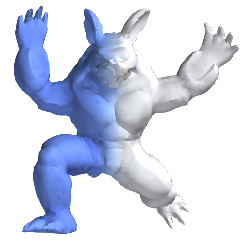
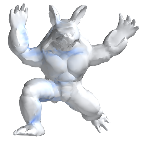
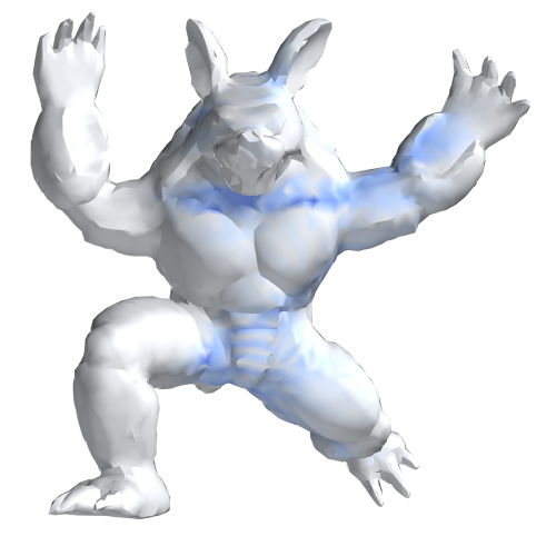
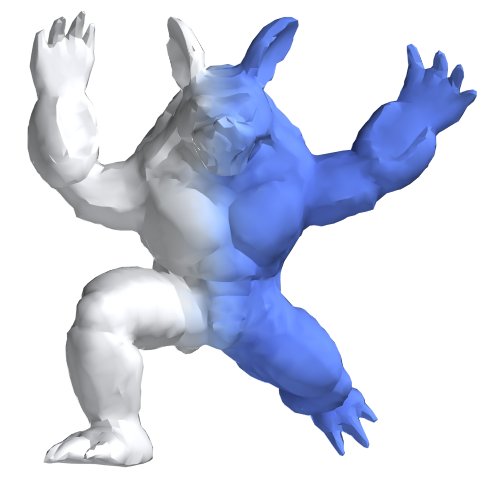
$\alpha=10^{-2}$
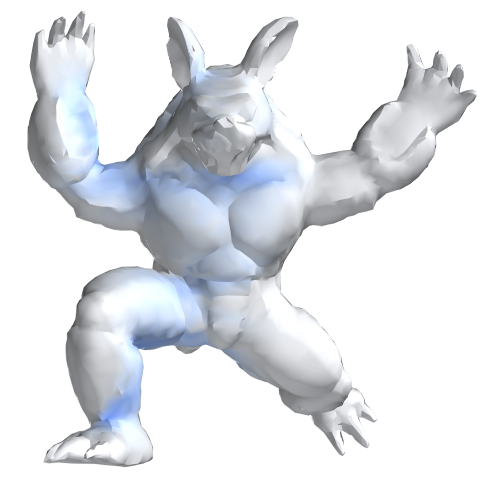
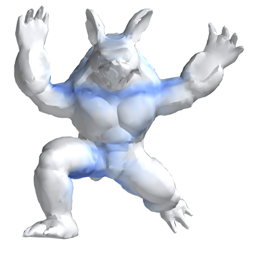
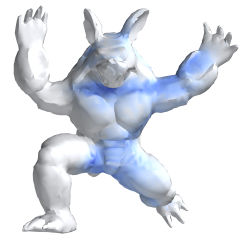
$\alpha=10^{-1}$
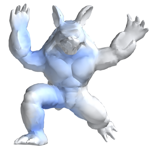
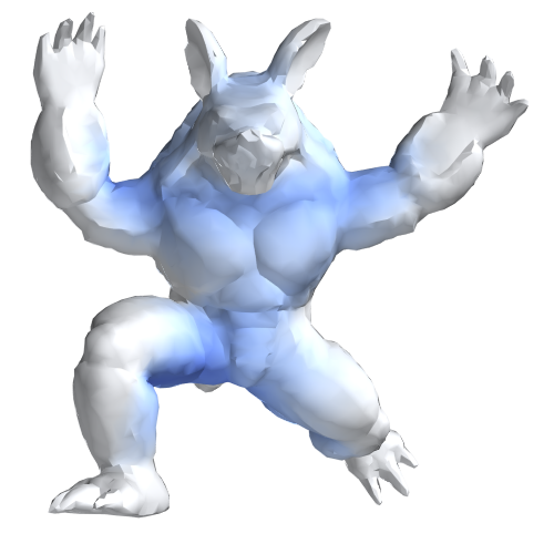
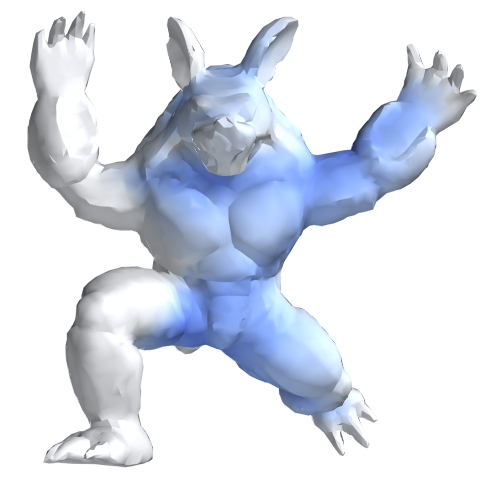
$\alpha=1$
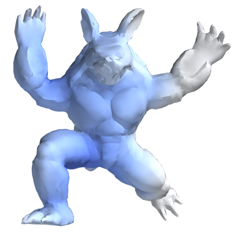
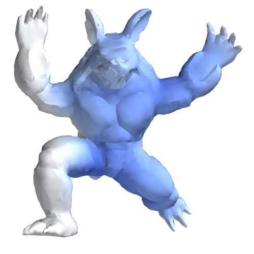
	$t=0$	$t=\nicefrac{{1}}{{4}}$	$t=\nicefrac{{1}}{{2}}$	$t=\nicefrac{{3}}{{4}}$	$t=1$

Figure 7. Effect of the regularizing parameter $\alpha$ penalizing congestion. On each row, the interpolation between the same boundary data (distributions located on the right and on the left of the armadillo) is shown. Different rows correspond to different to different values of $\alpha$. The color in each image is normalized independently from the others, explaining the change in intensity. Mass is always preserved along the interpolation.

In optimal transport there is no price paid for highly-congested densities. Imagine the probability distributions as an assembly of particles moving along the surface. Along a geodesic in Wasserstein space, each particle evolves in time by following a geodesic on the surface—but does not feel the presence of its neighbors.

Now imagine, due to the particular structure of the triangle mesh, there is a small shortcut in terms of geodesic distance through which all geodesics tend to concentrate. This is likely to appear near a hyperbolic vertex [Polthier and Schmies, 2006]. Then all the particles have the incentive to take this shortcut, resulting in densely-populated zones, as they are not prone to congestion. As an example, see the first row of Figure 7 in which, to go from the left to the right of the armadillo, all the particles go through only two paths, leaving the rest of the mesh without any mass.

This effect, although visually unpleasant, would be observed on a smooth surface $\mathcal{M}$ as soon as geodesics concentrate in some regions. A way to remove this artifact is to penalize congestion; we can do so with little modification to the algorithm.

We penalize the densities by their $L^{2}$ norms: The choice of the exponent $2$ is important, as it preserves the quadratic structure of the optimization problem. Namely, we add to the Lagrangian (20) the term

(24) $$\frac{\alpha\tau}{2}\sum_{t\in\mathcal{G}_{\text{time}}^{\text{c}}}\sum_{v\in V}|v||\mu^{t}_{v}|^{2}=\sup_{\lambda}\sum_{t\in\mathcal{G}_{\text{time}}^{\text{c}}}\sum_{v\in V}\tau|v|\left(\lambda^{t}_{v}\mu_{v}^{t}-\frac{1}{2\alpha}(\lambda_{v}^{t})^{2}\right),$$

where the parameter $\alpha$ tunes the scale of the congestion effect and $\lambda\in\mathbb{R}^{\mathcal{G}_{\text{time}}^{\text{c}}\times V}$ corresponds to the dual variable associated to the congestion constraint.

Using the notation from Section 4.2, one can write the problem as maximizing

(25) $$\max_{\hat{\Lambda}(\varphi,\lambda)=q}F(\varphi,\lambda)+C(q),$$

but this time

(26) $$F(\varphi,\lambda)=\eqref{equation_definition_F}-\frac{1}{2\alpha}\sum_{t\in\mathcal{G}_{\text{time}}^{\text{c}}}\sum_{v\in V}\tau|v|(\lambda_{v}^{t})^{2}$$

and $\hat{\Lambda}(\varphi,\lambda)=(-\lambda,0)-\Lambda(\varphi)$. Then one runs exactly the same algorithm, with a straightforward adaptation of the update formulas.

After regularization, the interpolation is no longer a geodesic. For instance, the interpolation between two instances of the same probability distribution is not constant in time, because the $L^{2}$ norm potentially can be reduced by diffusing outward in the intermediate time steps. On the other hand, undesirable sharp features and oscillations can be removed, as seen in Figure 7. Note that regardless of the level of regularization, the interpolating curves are still valued in $\mathcal{P}(S)$, i.e. mass is still preserved along the interpolation.

The tuning of the parameter $\alpha$ allows our method to be robust to noisy mesh inputs, as shown in Figure 8. Noisy meshes have more local variation in curvature, leading to a higher tendency for congested trajectories, but this can be tamed via greater regularization.

Recall that the dynamical formulation of optimal transport can be interpreted as the least-action principle for a pressureless gas. The effect of the penalization of congested densities can be seen, from the modeling point of view, as adding a pressure force: the trajectories of the moving particles are no longer geodesics, they are bent by the pressure forces. The congestion term can also be see as an instance of variational mean field games, for which the augmented Lagrangian approach has been applied for flat spaces with grid discretization [Benamou et al., 2017].

Rather than a drawback, we see the regularization as an added feature of our method. Without regularization, one has a faithful discrete Benamou–Brenier formula on discrete surfaces with Riemannian structure. For applications in physics or gradient flows (Subsection 6.2), this is likely the preferable formulation. For graphics, where blurriness might be sharpened a posteriori, penalizing concentration of mass is reasonable. Either can be achieved thanks to our regularization term without additional computational cost and only by adding a few lines of code.

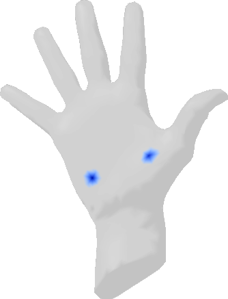
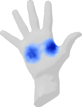
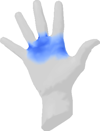
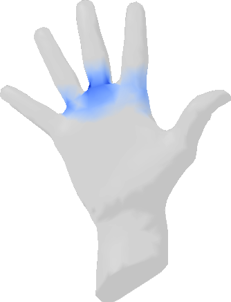
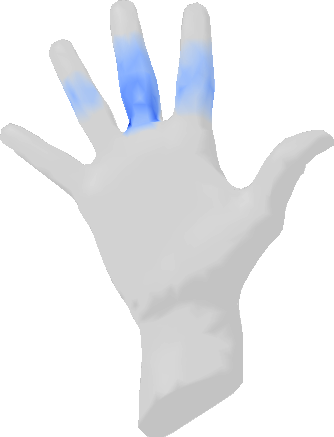
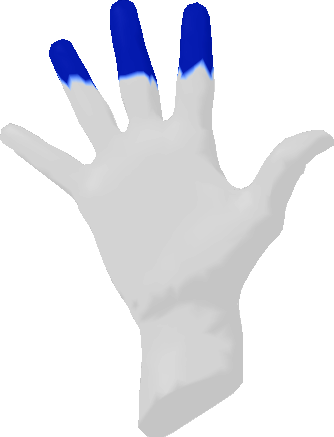
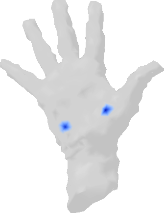
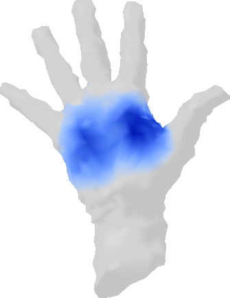
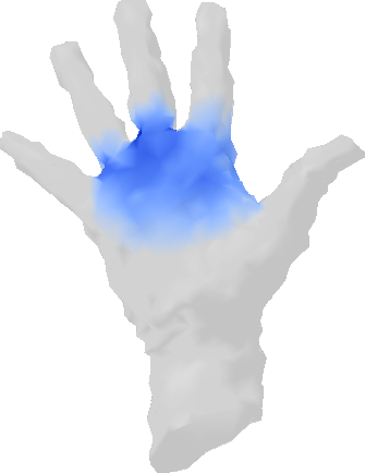
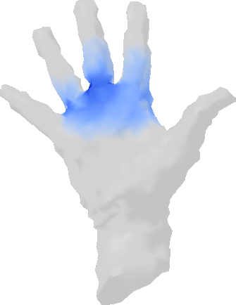
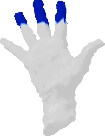
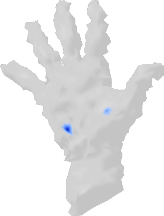
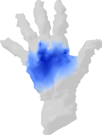
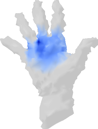
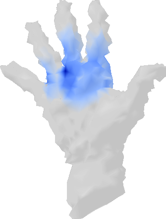
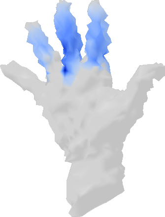
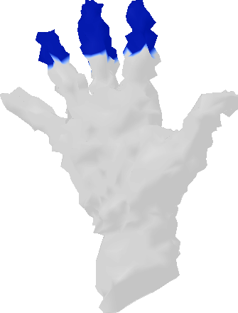
$t=0$	$t=\nicefrac{{1}}{{5}}$	$t=\nicefrac{{2}}{{5}}$	$t=\nicefrac{{3}}{{5}}$	$t=\nicefrac{{4}}{{5}}$	$t=1$

Figure 8. Robustness to noisy meshes, after adjusting the parameter $\alpha$. Top row: original mesh, $\alpha=0.02$; middle row: noisy mesh, $\alpha=0.1$; bottom row: very noisy mesh, $\alpha=0.2$. The bounding boxes of the meshes were of side length ~1.5. Noisy mesh vertices were obtained by uniformly random perturbation, in the normal direction, of magnitudes up to 0.02 and 0.04, for the middle and bottom row, respectively.

5.5. Intrinsic geometry

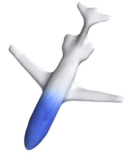
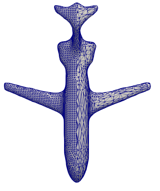
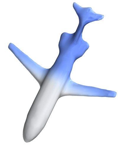
$t=0$	mesh	$t=1$
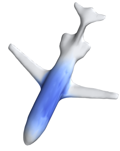
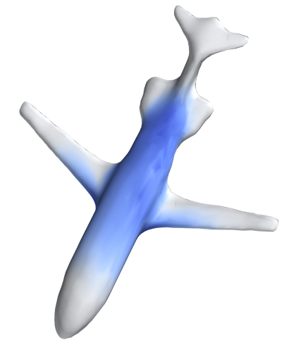
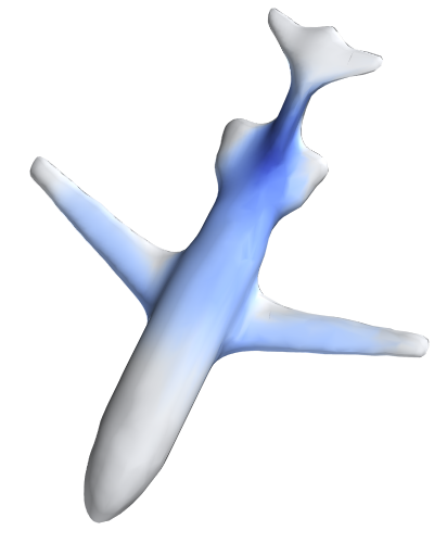
$t=\nicefrac{{1}}{{4}}$	$t=\nicefrac{{1}}{{2}}$	$t=\nicefrac{{3}}{{4}}$

Figure 9. Top row: mesh and initial/final probability distributions. Notice the difference of coarseness in the mesh. Bottom row: interpolation shown at different times where no effect of the difference in coarseness is seen. We have used the regularization described in Subsection 5.4 with $\alpha=0.1$.

To illustrate the fact that the discrete Wasserstein metric is really associated to the geometric structure of the mesh, we perform the following experiment. We design a mesh where the right part is much coarser than the left one, and we let the density evolve. As one can see in Figure 9, the jump in coarseness does not affect the density and does not produce any numerical artifact.

5.6. Arbitrary topologies

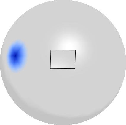
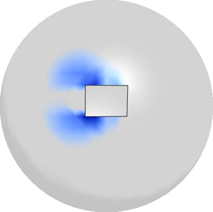
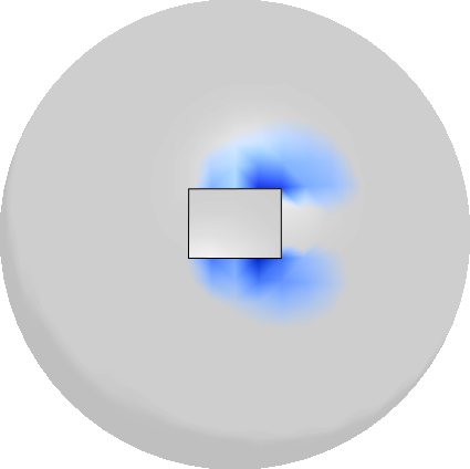
$t=0$	$t=\nicefrac{{1}}{{3}}$	$t=\nicefrac{{2}}{{3}}$	$t=1$

Figure 10. Our formulation easily handles non-spherical topologies. In the top row is a punctured sphere, and in the bottom row is a genus-1 teapot mesh. These interpolations were generated with $\alpha=0.02$ and $\alpha=0.2$, respectively.

The discrete formulation that we have chosen applies without change to meshes with boundary and those of non-spherical topology. This is illustrated in Figure 10 with two meshes topologically equivalent to a disc and a torus.

In the first example, the interpolating distribution stays near the boundary, approximately following the geodesic between the means of the endpoint distributions. In the second example, one can see the initial distribution splitting to travel both ways to the other side of a handle, before merging again to achieve the final distribution.

5.7. Comparison to convolutional method

Solomon et al. [2015] provide a convolutional method for approximating the Wasserstein geodesic between two distributions supported on triangle meshes. Their approach solves a regularized optimal transport barycenter problem using a modified Sinkhorn algorithm, with a heat kernel taking the place of explicitly-calculated pairwise distances between vertices. As a result, their method blurs the input distributions, and the interpolated distributions are typically of higher entropy than the endpoints. This is combated with a nonconvex projection method that attempts to lower the entropy of intermediate distributions to an approximated bound.

In comparing our methods, we found that [Solomon et al., 2015] also tends to produce interpolating distributions that do not travel with constant speed. This effect can be seen in Figures 11 and 12, where their interpolating distributions remain mostly stationary for times near $t=0$ and $t=1$, but move with high speed for times near $t=\nicefrac{{1}}{{2}}$. Loosening the entropy bound in the nonconvex step helps somewhat, but the problem persists regardless. Most likely this effect is due to the fact that the entropy reduction step of their algorithm is not geometry-aware but rather simply sharpens the regularized interpolant.

Our method does not suffer from this issue, and the spread of our interpolating distributions is comparable or better in both cases. Furthermore, unless the regularizer $\alpha$ is large, our interpolating distributions tend to diffuse only in the direction of the geodesics along which particles are traveling, which better mimics the behavior of Wasserstein geodesics; this diffusion is reduced by adding more time steps to our interpolation problem.

Our formulation also has comparable runtimes to the convolutional method of Solomon et al. [2015]. For instance, the implementation of the convolutional method provided by the authors of that paper took 57 and 141 seconds to converge, on the punctured sphere (1020 vertices) and teapot (3900 vertices), respectively, for 13 time steps. This is to be put in comparision with the timings provided in Subsection 5.2.

The comparisons in this section were computed on a 3.60GHz Intel i7-7700 processor with 32GB of RAM. For the convolutional method, the heat kernel was used to diffuse to $t=0.0015$ with 10 implicit Euler steps.

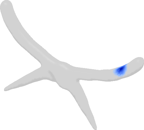
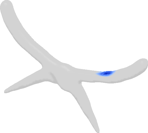
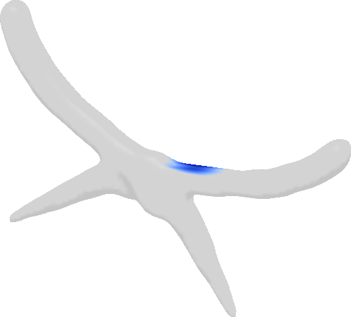
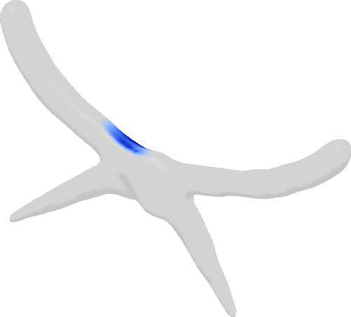
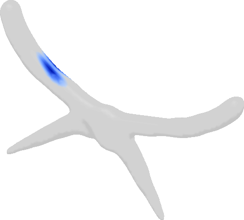
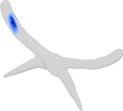
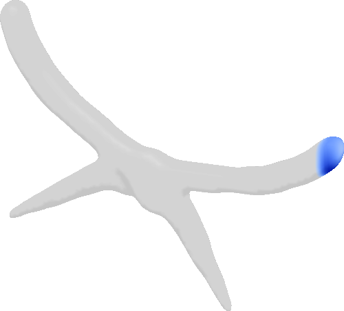
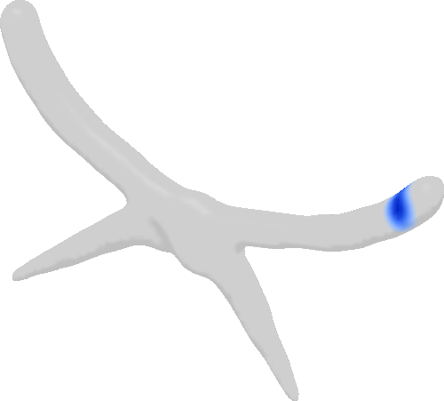
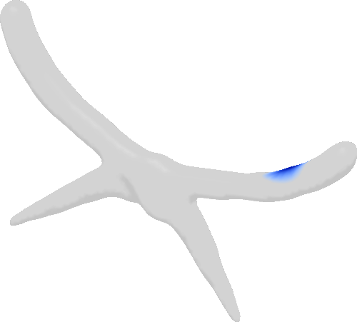
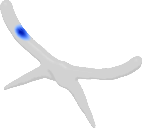
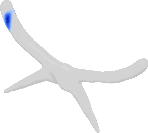
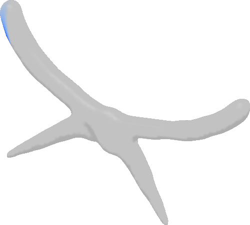
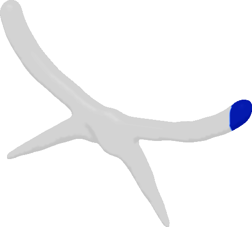
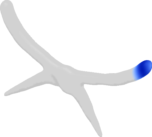
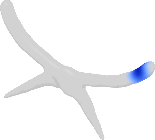
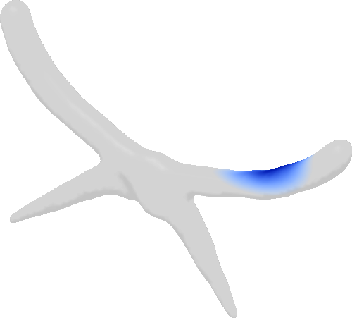
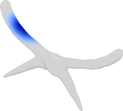
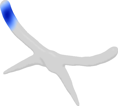
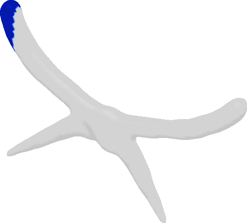
$t=0$	$t=\nicefrac{{1}}{{7}}$	$t=\nicefrac{{2}}{{7}}$	$t=\nicefrac{{3}}{{7}}$	$t=\nicefrac{{4}}{{7}}$	$t=\nicefrac{{5}}{{7}}$	$t=\nicefrac{{6}}{{7}}$	$t=1$

Figure 11. Constant-speed interpolation. Indicator distributions on handle ends of a pliers mesh are interpolated. Top row: our method, calculated with $\alpha=0.001$; middle row: method of Solomon et al. [2015], calculated with entropy bounded by that of the endpoint distributions; bottom row: method of Solomon et al. [2015], calculated with no entropy bound. As can be seen, the method of Solomon et al. [2015] stays mostly stationary except for the middle frames.

$t=0$	$t=\nicefrac{{1}}{{7}}$	$t=\nicefrac{{2}}{{7}}$	$t=\nicefrac{{3}}{{7}}$	$t=\nicefrac{{4}}{{7}}$	$t=\nicefrac{{5}}{{7}}$	$t=\nicefrac{{6}}{{7}}$	$t=1$

Figure 12. Constant-speed interpolation. Delta distributions on a horse mesh are interpolated. Top row: our method, calculated with $\alpha=0.01$; middle row: method of Solomon et al. [2015], calculated with entropy bounded by that of endpoint distributions; bottom row: method of Solomon et al. [2015], calculated with no entropy bound. For the middle row, the motion is even more concentrated in the middle frames. As seen in the bottom row, exclusion of the entropy bound helps somewhat, but the result still is mostly stationary, save for the middle frames.

6. Applications and extensions

6.1. Harmonic mappings

Figure 13. (a) Data: boundary conditions, i.e. value of the probability distributions at the boundary vertexes of a regular triangulation of an equilateral triangle. (b) Result: interpolation over the interior of the triangular mesh obtained by minimizing the Dirichlet energy with the boundary constraints. The mesh of the source domain $\Omega$ is a regular triangulation of a triangle with $15$ vertexes per side but for clarity reasons we display the value of the probability distributions only a subset of the set of vertexes. The target domain $\mathcal{M}$ is a flat square triangulated with $30$ vertexes by side.

As $\mathcal{P}(\mathcal{M})$ can be viewed as a Riemannian manifold of infinite dimension, one can consider not only geodesics valued in this space, but also harmonic mappings. That is, we consider a domain $\Omega$ and a function $\mu:x\in\Omega\to\mu^{x}$ which takes fixed values on $\partial\Omega$ the boundary of $\Omega$ and minimizes the Dirichlet energy

(27) $$\mathrm{Dir}(\mu):=\frac{1}{2}\int_{\Omega}\|\nabla_{\Omega}\mu^{x}\|^{2}_{T_{\mu^{x}}\mathcal{P}(\mathcal{M})}\mathrm{d}x,$$

where the norm $\|\ \|_{\mu^{x}}$ is defined in (5). Such harmonic mappings have been introduced under the name soft maps by Solomon et al. [2012; 2013] for the purpose of surface mapping; one can also find a formal definition and theoretical analysis in [Lavenant, 2017; Lu, 2017].

As explained by Lavenant [2017], if some boundary conditions $\bar{\mu}:\partial\Omega\to\mathcal{P}(\mathcal{M})$ are given, the Dirichlet problem consists in minimizing the Dirichlet energy (27) of $\mu$ under the constraint that $\mu=\bar{\mu}$ on $\partial\Omega$. Specifically, it is a convex problem whose dual reads

(28) $$\begin{cases}\max_{\varphi}&\int_{\partial\Omega}\left(\int_{\mathcal{M}}\varphi(x,\cdot)\cdot n_{\Omega}(x)\mathrm{d}\bar{\mu}^{x}\right)\mathrm{d}x\\ &\text{s.t. }\nabla_{\Omega}\cdot\varphi+\frac{1}{2}\|\nabla_{\mathcal{M}}\varphi\|^{2}\leqslant 0\text{ on }\Omega\times\mathcal{M},\end{cases}$$

where $\varphi$ is defined on $\Omega\times M$ and valued in $T\Omega$ (i.e. for a point $(x,y)\in\Omega\times M$, one has $\varphi(x,y)\in T_{x}\Omega$), $n_{\Omega}(x)$ is the outward normal to $\Omega$, and $\mathrm{d}x$ is the integration on $\partial\Omega$ w.r.t. the surface measure. In the case where $\Omega$ is a segment, the dual problem (3) for the geodesics is recovered.

To discretize (28), we use the same strategy as for the geodesic problem. We assume that we have $S_{\Omega}=(V_{\Omega},E_{\Omega},T_{\Omega})$ a triangulation of the surface $\Omega$. The discrete unknown $\varphi$ maps every element of $T_{\Omega}\times V$ onto a vector in $\mathbb{R}^{3}$ (thought as the tangent space of $S_{\Omega}$). The divergence $\nabla_{\Omega}\cdot\varphi$ is replaced by its discrete counterpart which lives on $V_{\Omega}\times V$. On the other hand, $\nabla_{\mathcal{M}}\varphi$ is naturally seen as a vector in $\mathbb{R}^{3}$ for each pair of triangles in $T_{\Omega}\times T$. We apply the same idea: For the term $\|\nabla_{\mathcal{M}}\varphi\|^{2}$, first square and then average (weighting by the area of the triangles) to put it on the grid $V_{\Omega}\times V$. Once we have a fully-discrete problem, we build an augmented Lagragian and use ADMM: The solution $\mu$ is the Lagrange multiplier associated to the constraint $A=\nabla_{\Omega}\cdot\varphi$.

In Figure 13, we show an example where $S_{\Omega}$ is a triangulation of an equilateral triangle and $S$ the triangulation of a flat square. On the corners of the triangle we put some distributions, and on the side, as part of the boundary data, we have chosen to put the geodesic in the Wasserstein space between the distributions on the corners. This choice is arbitrary, we could have chosen other configurations on the edges of the boundary of the triangle $\Omega$. This picture resembles the barycentric interpolation [Cuturi and Doucet, 2014; Benamou et al., 2015; Solomon et al., 2015], though no theoretical evidence indicates that harmonic and barycentric interpolation coincide.

6.2. Gradient flows in the Wasserstein space

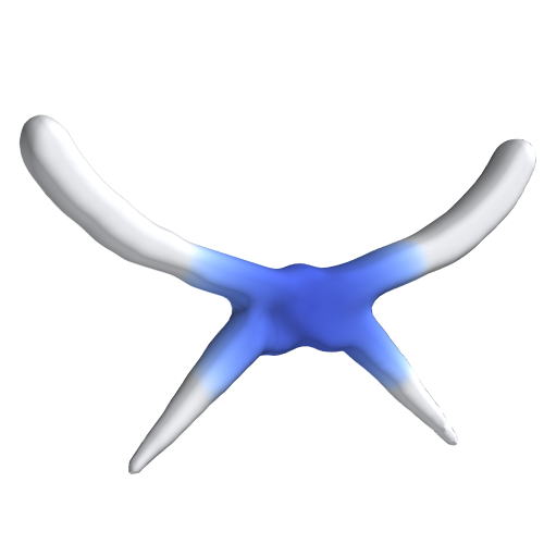
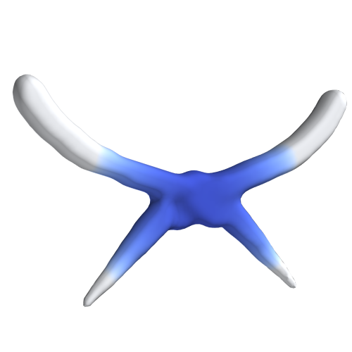
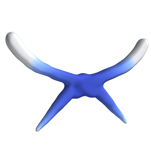
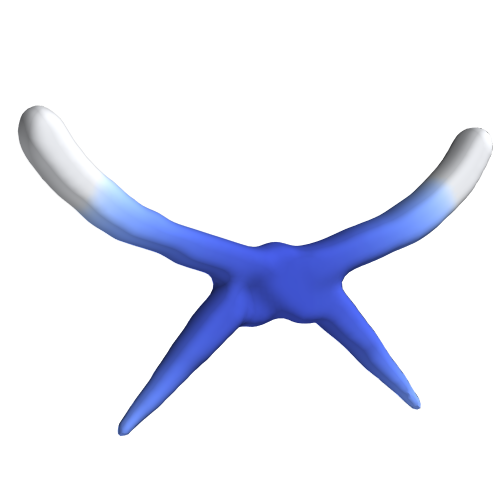
$t=0$	$t=1$	$t=2$	$t=3$	$t=4$	$t=5$	$t=6$	$t=7$

Figure 14. First row: gradient flow in discrete Wasserstein space of the functional (32).The potential is chosen to be $W(x,y,z)=z$: the mass flows down and then saturates because of the density constraint. Congestion can be observed as the mass goes through the thinner part. Second row: gradient flow of the internal energy (33) starting from a delta function on the surface of the plier. The colors do not correspond to the same scale for different times; otherwise nothing would be seen for $t>0$ thanks to the peaked distribution at $t=0$. Notice the finite speed of propagation of the density.

The seminal work of Jordan et al. [1998], demonstrates that by considering the gradient flow

(29) $$\partial_{t}\mu^{t}=-\nabla_{\mathcal{P}(M)}F(\mu^{t}),$$

where $\nabla_{\mathcal{P}(M)}$ is the gradient w.r.t. the scalar product defined by (4) and (5), one can recover several well-known PDE (Fokker–Planck, porous medium equations, aggregation diffusion equations) by an appropriate choice of the functional $F:\mathcal{P}(M)\to\mathbb{R}$ [Ambrosio et al., 2008; Santambrogio, 2015]. Moreover, a natural implicit discretization comes with this equation: The idea is to take a time step $s>0$ and to define $\mu^{ks}$ for $k=0,1,\ldots$ recursively in the following way:

(30) $$\mu^{(k+1)s}:=\operatorname*{arg\,min}_{\mu}\left[\frac{W_{2}^{2}(\mu,\mu^{ks})}{2s}+F(\mu)\right].$$

The scheme above, defined in arbitrary metric spaces, is refered to as minimizing movement scheme, in the framework of optimal transport it is sometimes known as a JKO integrator, after the work of Jordan, Kinderlehrer and Otto [1998].

In the case of a discrete surface $S$ with the Riemannian structure on $\mathcal{P}(S)$, (29) makes sense and can be written

(31) $$\partial_{t}\mu^{t}=-(P_{\mu^{t}})^{-1}\nabla F(\mu^{t})$$

where $P_{\mu}$ is the metric tensor defined in (14) and $\nabla F$ is the usual gradient of $F$ as a function from $\mathbb{R}^{|V|}$ to $\mathbb{R}$. We can still define an iterative scheme to compute solutions of (31) by solving (30), where $W_{2}$ has been replaced by the discrete Wasserstein distance $W_{d}$. As long as $F:\mathcal{P}(S)\to\mathbb{R}$ is convex, the discrete version of (30) can be tackled by the same augmented Lagrangian and ADMM iterations at the price of introducing an additional variable [Benamou et al., 2016].

We cannot recover cotangent Laplacian heat flow as a gradient flow for the Wasserstein distance $W_{d}$; to get such a result, one would need to define $\hat{\mu}$ by some nonlinear averaging process rather than (10). Such a choice would increase the complexity of computing geodesics, and it would be likely to introduce more diffusion as in [Maas, 2011; Erbar et al., 2017].

The advantages of our numerical method are that positivity is automatic and that mass is preserved. Moreover, as we expect the difference between two solutions $\mu^{ks}$ and $\mu^{(k+1)s}$ to be very small, we do not need a large number of discretization points in time $N$ (we chose $N=5$ in practice) for the computation of the discrete Wasserstein distance.

We apply our model to two different cases, illustrated in Figure 14. The first corresponds to

(32) $$F(\mu)=\begin{cases}\sum_{v\in V}|v|W_{v}\mu_{v}&\text{if }\mu_{v}\leqslant\mu^{\star}\ \forall v\in V,\\ +\infty&\text{else},\end{cases}$$

where $W$ contains one value per vertex. This choice of $F$ yields a crowd motion model [Maury et al., 2010; Santambrogio, 2018]: The probability distribution wants to flow to the areas where $W$ is low, but at the same time its density is constrained to stay below a threshold $\mu^{\star}$. This model can only be formulated in terms of a gradient flow in Wasserstein space and not as an evolution PDE, justifying the use of a JKO integrator. The second corresponds to

(33) $$F(\mu)=\frac{1}{m-1}\sum_{v\in V}|v|(\mu_{v})^{m}.$$

In the case of a continuous manifold $\mathcal{M}$, this choice of $F$ yields the porous medium equation $\partial_{t}\mu=\Delta(\mu^{m})$ [Vázquez, 2007]. With the scheme (30), we do not recover a discrete cotangent Laplacian, but the computed solution still exhibits features of the porous medium, like a finite speed of propagation and a convergence to a uniform probability distribution.

7. Discussion and conclusion

Although techniques using entropic regularization or semi-discrete optimal transport can interpolate between distributions on a discrete surface, they do not provide a Riemannian structure and are subject to practical limitations that restrict the scenarios to which they can be applied. Using an intrinsic formulation of dynamical transport, we can realize the theoretical and practical potential of optimal transport on discrete domains enabled by the Riemannian structure on the space of probability distributions, the so-called Otto calculus. Our technique can be phrased in familiar language from discrete differential geometry and is implementable using standard tools in that domain. The key ingredients, namely first- and second-order operators in geometry processing (gradient, divergence, Laplacian) as well as SOCP optimization, remain in the realm of what is already widely used.

We have demonstrated the power of our model by showing how it can handle a variety of geometries and peaked distributions, while introducing little diffusion. Mass may concentrate to yield a visually inelegant result, but this behavior is at the core of optimal transport theory and expected: No price is paid for mass congestion, and hence any concentration of geodesics will result in a concentration of mass. Nevertheless, as we have shown, one can easily modify the optimization problem to penalize congested densities, leading to smoother interpolants with a controllable level of diffusion. Unlike entropically-regularized transport, however, our optimization problem does not degenerate as the coefficient in front of the regularizer vanishes.

Beyond evaluation of transport distances, our framework extends to support other tasks involving transport terms. We can reliably compute harmonic mappings valued in this discrete Wasserstein space, and the JKO integrator based on our discrete Wasserstein distance exhibits expected qualitative behavior.

The main drawback of our approach remains its scalability. The bottleneck of the computations is the solution of a linear system whose number of unknowns is the product of the number of discretization points in time and the size of the mesh. This is an extremely structured linear system on a product manifold, for which specialized matrix inversion techniques may exist. In any event, with the current bottleneck our method can handle meshes with few thousand vertices but is not currently practical for larger meshes.

As one of the first structure-preserving discretizations of transport on meshes, our work also suggests several exciting avenues for future research. Many theoretical properties of our discrete Wasserstein distance remain to be explored. For instance, while we have shown that our formulation is a true Riemannian distance, one could verify the extent to which a wealth of other theoretical properties of transport are preserved. Convergence of our transport over meshes to the true transport in the limit of mesh refinement also remains an open problem for our techniques and others in a similar class. From a practical perspective, a natural next step is to accelerate the optimization procedure as much as possible; a faster solver for the convex optimization problem would clearly benefit our method.

References

- [1]
- Ambrosio et al. [2008] Luigi Ambrosio, Nicola Gigli, and Giuseppe Savaré. 2008. Gradient Flows: In Metric Spaces and in the Space of Probability Measures. Springer Science & Business Media.
- Aurenhammer et al. [1998] Franz Aurenhammer, Friedrich Hoffmann, and Boris Aronov. 1998. Minkowski-type theorems and least-squares clustering. Algorithmica 20, 1 (1998), 61–76.
- Azencot et al. [2016] Omri Azencot, Orestis Vantzos, and Mirela Ben-Chen. 2016. Advection-based function matching on surfaces. In Computer Graphics Forum, Vol. 35. Wiley Online Library, 55–64.
- Benamou and Brenier [2000] Jean-David Benamou and Yann Brenier. 2000. A computational fluid mechanics solution to the Monge-Kantorovich mass transfer problem. Numer. Math. 84, 3 (2000), 375–393.
- Benamou and Carlier [2015] Jean-David Benamou and Guillaume Carlier. 2015. Augmented Lagrangian methods for transport optimization, mean field games and degenerate elliptic equations. Journal of Optimization Theory and Applications 167, 1 (2015), 1–26.
- Benamou et al. [2015] Jean-David Benamou, Guillaume Carlier, Marco Cuturi, Luca Nenna, and Gabriel Peyré. 2015. Iterative Bregman projections for regularized transportation problems. SIAM Journal on Scientific Computing 37, 2 (2015), A1111–A1138.
- Benamou et al. [2016] Jean-David Benamou, Guillaume Carlier, and Maxime Laborde. 2016. An augmented Lagrangian approach to Wasserstein gradient flows and applications. ESAIM: Proceedings and Surveys 54 (2016), 1–17.
- Benamou et al. [2017] Jean-David Benamou, Guillaume Carlier, and Filippo Santambrogio. 2017. Variational mean field games. In Active Particles, Volume 1. Springer, 141–171.
- Bonneel et al. [2011] Nicolas Bonneel, Michiel Van De Panne, Sylvain Paris, and Wolfgang Heidrich. 2011. Displacement interpolation using Lagrangian mass transport. In ACM Transactions on Graphics (TOG), Vol. 30. ACM, 158.
- Boyd et al. [2011] Stephen Boyd, Neal Parikh, Eric Chu, Borja Peleato, Jonathan Eckstein, et al. 2011. Distributed optimization and statistical learning via the alternating direction method of multipliers. Foundations and Trends in Machine Learning 3, 1 (2011), 1–122.
- Boyd and Vandenberghe [2004] Stephen Boyd and Lieven Vandenberghe. 2004. Convex Optimization. Cambridge University Press.
- Brenier [1991] Yann Brenier. 1991. Polar factorization and monotone rearrangement of vector-valued functions. Communications on Pure and Applied Mathematics 44, 4 (1991), 375–417.
- Brenner and Scott [2007] Susanne Brenner and Ridgway Scott. 2007. The Mathematical Theory of Finite Element Methods. Vol. 15. Springer Science & Business Media.
- Chow et al. [2016] Shui-Nee Chow, Luca Dieci, Wuchen Li, and Haomin Zhou. 2016. Entropy dissipation semi-discretization schemes for Fokker-Planck equations. arXiv:1608.02628 (2016).
- Claici et al. [2018] Sebastian Claici, Edward Chien, and Justin Solomon. 2018. Stochastic Wasserstein barycenters. In Proceedings of the 35th International Conference on Machine Learning, ICML 2018 (to appear).
- Cuturi [2013] Marco Cuturi. 2013. Sinkhorn distances: Lightspeed computation of optimal transport. In Advances in Neural Information Processing Systems, NIPS 2013. 2292–2300.
- Cuturi and Doucet [2014] Marco Cuturi and Arnaud Doucet. 2014. Fast computation of Wasserstein barycenters. In International Conference on Machine Learning. 685–693.
- De Goes et al. [2012] Fernando De Goes, Katherine Breeden, Victor Ostromoukhov, and Mathieu Desbrun. 2012. Blue noise through optimal transport. ACM Transactions on Graphics (TOG) 31, 6 (2012), 171.
- de Goes et al. [2011] Fernando de Goes, David Cohen-Steiner, Pierre Alliez, and Mathieu Desbrun. 2011. An optimal transport approach to robust reconstruction and simplification of 2d shapes. In Computer Graphics Forum, Vol. 30. Wiley Online Library, 1593–1602.
- de Goes et al. [2015a] Fernando de Goes, Mathieu Desbrun, and Yiying Tong. 2015a. Vector field processing on triangle meshes. In SIGGRAPH Asia 2015 Courses. ACM, 17.
- de Goes et al. [2014] Fernando de Goes, Pooran Memari, Patrick Mullen, and Mathieu Desbrun. 2014. Weighted Triangulations for Geometry Processing. ACM Trans. Graph. 33, 3 (June 2014), 28:1–28:13.
- de Goes et al. [2015b] Fernando de Goes, Corentin Wallez, Jin Huang, Dmitry Pavlov, and Mathieu Desbrun. 2015b. Power particles: an incompressible fluid solver based on power diagrams. ACM Trans. Graph. 34, 4 (2015), 50–1.
- Digne et al. [2014] Julie Digne, David Cohen-Steiner, Pierre Alliez, Fernando De Goes, and Mathieu Desbrun. 2014. Feature-preserving surface reconstruction and simplification from defect-laden point sets. Journal of Mathematical Imaging and Vision 48, 2 (2014), 369–382.
- Edmonds and Karp [1972] Jack Edmonds and Richard M Karp. 1972. Theoretical improvements in algorithmic efficiency for network flow problems. Journal of the ACM (JACM) 19, 2 (1972), 248–264.
- Erbar et al. [2017] Matthias Erbar, Martin Rumpf, Bernhard Schmitzer, and Stefan Simon. 2017. Computation of Optimal Transport on Discrete Metric Measure Spaces. arXiv:1707.06859 (2017).
- Gallouët and Mérigot [2017] Thomas O Gallouët and Quentin Mérigot. 2017. A Lagrangian scheme à la Brenier for the incompressible Euler equations. Foundations of Computational Mathematics (2017), 1–31.
- Gangbo and McCann [1996] Wilfrid Gangbo and Robert J McCann. 1996. The geometry of optimal transportation. Acta Mathematica 177, 2 (1996), 113–161.
- Gigli and Maas [2013] Nicola Gigli and Jan Maas. 2013. Gromov–Hausdorff convergence of discrete transportation metrics. SIAM Journal on Mathematical Analysis 45, 2 (2013), 879–899.
- Gladbach et al. [2018] Peter Gladbach, Eva Kopfer, and Jan Maas. 2018. Scaling limits of discrete optimal transport. arXiv:1809.01092 (2018).
- Grant and Boyd [2008] Michael Grant and Stephen Boyd. 2008. Graph implementations for nonsmooth convex programs. In Recent Advances in Learning and Control, V. Blondel, S. Boyd, and H. Kimura (Eds.). Springer-Verlag Limited, 95–110.
- Grant and Boyd [2014] Michael Grant and Stephen Boyd. 2014. CVX: Matlab Software for Disciplined Convex Programming, version 2.1. http://cvxr.com/cvx.
- Guittet [2003] Kevin Guittet. 2003. On the time-continuous mass transport problem and its approximation by augmented Lagrangian techniques. SIAM J. Numer. Anal. 41, 1 (2003), 382–399.
- Heeren et al. [2012] Behrend Heeren, Martin Rumpf, Max Wardetzky, and Benedikt Wirth. 2012. Time-Discrete Geodesics in the Space of Shells. In Computer Graphics Forum, Vol. 31. Wiley Online Library, 1755–1764.
- Hug et al. [2015] Romain Hug, Nicolas Papadakis, and Emmanuel Maitre. 2015. On the convergence of augmented Lagrangian method for optimal transport between nonnegative densities. (2015).
- Jordan et al. [1998] Richard Jordan, David Kinderlehrer, and Felix Otto. 1998. The variational formulation of the Fokker–Planck equation. SIAM Journal on Mathematical Analysis 29, 1 (1998), 1–17.
- Jost [2008] Jürgen Jost. 2008. Riemannian geometry and geometric analysis. Vol. 42005. Springer.
- Kantorovich [1942] Leonid V Kantorovich. 1942. On the translocation of masses. In Dokl. Akad. Nauk. USSR (NS), Vol. 37. 199–201.
- Kitagawa et al. [2016] Jun Kitagawa, Quentin Mérigot, and Boris Thibert. 2016. Convergence of a Newton algorithm for semi-discrete optimal transport. arXiv preprint arXiv:1603.05579 (2016).
- Klein [1967] Morton Klein. 1967. A primal method for minimal cost flows with applications to the assignment and transportation problems. Management Science 14, 3 (1967), 205–220.
- Lavenant [2017] Hugo Lavenant. 2017. Harmonic mappings valued in the Wasserstein space. arXiv:1712.07528 (2017).
- Lévy [2015] Bruno Lévy. 2015. A numerical algorithm for semi-discrete optimal transport in 3D. ESAIM: Mathematical Modelling and Numerical Analysis 49, 6 (2015), 1693–1715.
- Li et al. [2018] Wuchen Li, Ernest K Ryu, Stanley Osher, Wotao Yin, and Wilfrid Gangbo. 2018. A parallel method for earth mover’s distance. Journal of Scientific Computing 75, 1 (2018), 182–197.
- Lu [2017] Zhuoran Lu. 2017. Properties of Soft Maps on Riemannian Manifolds. Ph.D. Dissertation. New York University.
- Maas [2011] Jan Maas. 2011. Gradient flows of the entropy for finite Markov chains. Journal of Functional Analysis 261, 8 (2011), 2250–2292.
- Maury et al. [2010] Bertrand Maury, Aude Roudneff-Chupin, and Filippo Santambrogio. 2010. A macroscopic crowd motion model of gradient flow type. Mathematical Models and Methods in Applied Sciences 20, 10 (2010), 1787–1821.
- McCann [1997] Robert J McCann. 1997. A convexity principle for interacting gases. Advances in Mathematics 128, 1 (1997), 153–179.
- Mérigot [2011] Quentin Mérigot. 2011. A multiscale approach to optimal transport. In Computer Graphics Forum, Vol. 30. Wiley Online Library, 1583–1592.
- Mérigot et al. [2018] Quentin Mérigot, Jocelyn Meyron, and Boris Thibert. 2018. An algorithm for optimal transport between a simplex soup and a point cloud. SIAM Journal on Imaging Sciences 11, 2 (2018), 1363–1389.
- Mérigot and Mirebeau [2016] Quentin Mérigot and Jean-Marie Mirebeau. 2016. Minimal geodesics along volume-preserving maps, through semidiscrete optimal transport. SIAM J. Numer. Anal. 54, 6 (2016), 3465–3492.
- MOSEK ApS [2017] MOSEK ApS. 2017. The MOSEK optimization toolbox for MATLAB manual.
- Orlin [1997] James B Orlin. 1997. A polynomial time primal network simplex algorithm for minimum cost flows. Mathematical Programming 78, 2 (1997), 109–129.
- Otto [2001] Felix Otto. 2001. The geometry of dissipative evolution equations: the porous medium equation. (2001).
- Panozzo et al. [2013] Daniele Panozzo, Ilya Baran, Olga Diamanti, and Olga Sorkine-Hornung. 2013. Weighted averages on surfaces. ACM Transactions on Graphics (TOG) 32, 4 (2013), 60.
- Papadakis et al. [2014] Nicolas Papadakis, Gabriel Peyré, and Edouard Oudet. 2014. Optimal transport with proximal splitting. SIAM Journal on Imaging Sciences 7, 1 (2014), 212–238.
- Pinkall and Polthier [1993] Ulrich Pinkall and Konrad Polthier. 1993. Computing discrete minimal surfaces and their conjugates. Experimental Mathematics 2, 1 (1993), 15–36.
- Polthier and Schmies [2006] Konrad Polthier and Markus Schmies. 2006. Straightest geodesics on polyhedral surfaces. ACM.
- Santambrogio [2015] Filippo Santambrogio. 2015. Optimal transport for applied mathematicians. Birkäuser, NY (2015), 99–102.
- Santambrogio [2018] Filippo Santambrogio. 2018. Crowd motion and evolution PDEs under density constraints.
- Solomon et al. [2015] Justin Solomon, Fernando De Goes, Gabriel Peyré, Marco Cuturi, Adrian Butscher, Andy Nguyen, Tao Du, and Leonidas Guibas. 2015. Convolutional Wasserstein distances: Efficient optimal transportation on geometric domains. ACM Transactions on Graphics (TOG) 34, 4 (2015), 66.
- Solomon et al. [2013] Justin Solomon, Leonidas Guibas, and Adrian Butscher. 2013. Dirichlet energy for analysis and synthesis of soft maps. In Computer Graphics Forum, Vol. 32. Wiley Online Library, 197–206.
- Solomon et al. [2012] Justin Solomon, Andy Nguyen, Adrian Butscher, Mirela Ben-Chen, and Leonidas Guibas. 2012. Soft maps between surfaces. In Computer Graphics Forum, Vol. 31. Wiley Online Library, 1617–1626.
- Solomon et al. [2014] Justin Solomon, Raif Rustamov, Leonidas Guibas, and Adrian Butscher. 2014. Earth mover’s distances on discrete surfaces. ACM Transactions on Graphics (TOG) 33, 4 (2014), 67.
- Trillos [2017] Nicolas Garcia Trillos. 2017. Gromov-Hausdorff limit of Wasserstein spaces on point clouds. arXiv:1702.03464 (2017).
- Vázquez [2007] Juan Luis Vázquez. 2007. The Porous Medium Equation: Mathematical Theory. Oxford University Press.
- Villani [2003] Cédric Villani. 2003. Topics in Optimal Transportation. Number 58. American Mathematical Soc.
- Villani [2008] Cédric Villani. 2008. Optimal Transport: Old and New. Vol. 338. Springer Science & Business Media.