Nonlinear transmission matrices of random optical media - Supplementary Information

S1 - Pump-Probe Optical Setup

The probe beam ($\lambda_{probe}=830~{}\rm{nm}$, MDL-III-830-800mW diode from Changchen New Industries Optoelectronics Technology Co., Ltd.) was polarized and collimated onto a spatial light modulator (SLM) (HSP512 from Boulder Nonlinear Systems). The image displayed on the SLM was relayed on the back aperture of a 30x ashperic lens ($f=6.2mm$), to focus the light on the sample. This configuration allowed correlating the change in phase of the pixels of the SLM to the direction of light impinging onto the sample Popoff et al. (2010). The scattered light was collected by a 20x objective from Newport ($f=9.0mm$, NA$=0.40$), with a field of view of $400~{}\rm{\mu m}$ in diameter, and imaged onto a CCD camera (Basler acA1920-25gm). To ensure the collection of only scattered photons, two cross polarizers were used on either side of the sample, with a measured fraction of collected light of 26%. The pump beam ($\lambda_{pump}=488~{}\rm{nm}$) was focused on the back focal plane of the input objective, creating a collimated beam $40\rm{\mu m}$ in width, collinear to the probe beam.

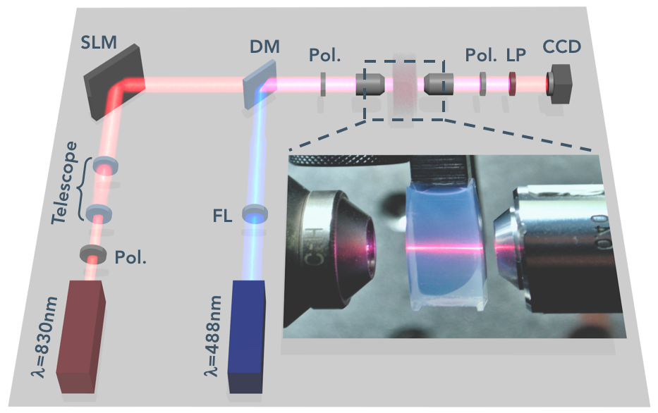
Figure 1: Pump-Probe Optical setup with wavefront shaping of the probe beam by SLM.

S2 - linear absorption of Silica Aerogel

The linear absorption of the used SA sample was estimated measuring the optical transmission of the sample for different angles and unpolarized, collimated light, and shown in fig. S2.

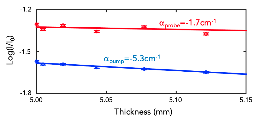
Figure 2: Transmission characteristics of the SA for the pump and probe wavelengths.

From the values of $\alpha$ it is possible to evaluate the scattering mean free path ($l_{pump}=1/\alpha_{pump}=1.9$ mm; $l_{probe}=1/\alpha_{probe}=5.9$ mm) and transport mean free path ($t_{pump}=l_{pump}/(1-g)=2.1$ mm; $t_{probe}=l_{probe}/(1-g)=6.5$ mm), where for the directionality factor we assumed the value $g=0.1$, as typical of silica aerogel samples Van de Hulst (1981). Therefore we can conclude that the experiments were completed in the weakly scattering regime.

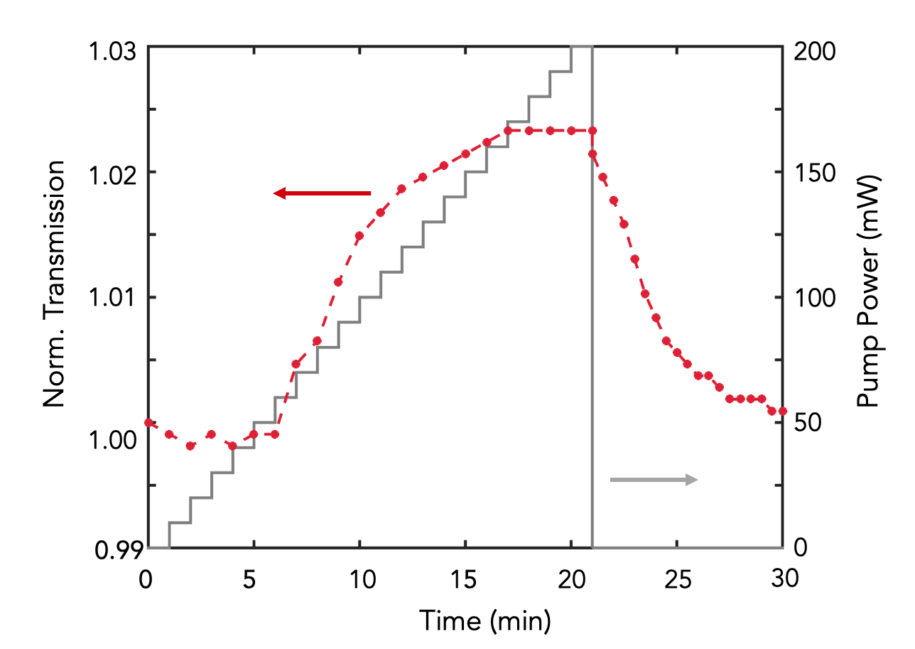
Figure 3: Transmission characteristics of the SA at the probe wavelength (left axis) and pump power (right axis) vs time.

To exclude pump induced absorption of the aerogel, we characterized the transmission of the sample at the probe wavelength vs time, for different values of the pump. Fig. S3 shows that the normalized transmission for a collimated probe increases marginally when the sample is collinearly pumped. This is in keeping with the fact that the aerogel has a defocusing nonlinearity, therefore it becomes slightly less dense, and thus less scattering medium.

S3 - Construction of the transmission matrices

The process for forming the TM from raw image data is outlined in figure S4. The 2D pixels of the CCD (M pixels) and of the SLM (N pixels) are mapped in a MxN TM matrix. To improve the SNR in the CCD images, we sum the total black-white intensity values over 8x8 pixels, giving a measurement range between 0 and 16383, rather than 0 to 255.

The phase of each pixel of the SLM is tuned in turn in the range $(-\pi,\pi)$, keeping the other pixels at $-\pi$ and the corresponding CCD image is acquired. The light impinging on the constant area of the SLM interferes with that of the tuned pixel, to access the complex values of the transmission channel. This process produces a stack of 3D images for each SLM pixel, as shown in panel c).

The intensity of each pixel in the stack changes with the phase of the SLM pixel in a cosine function. The amplitude and phase of the relative elements of the TM are given by the peak-to-peak value of the cosine function and by the offset respect to the reference phase, respectively, as seen in panels d-e). A typical complex TM is shown in panel f).

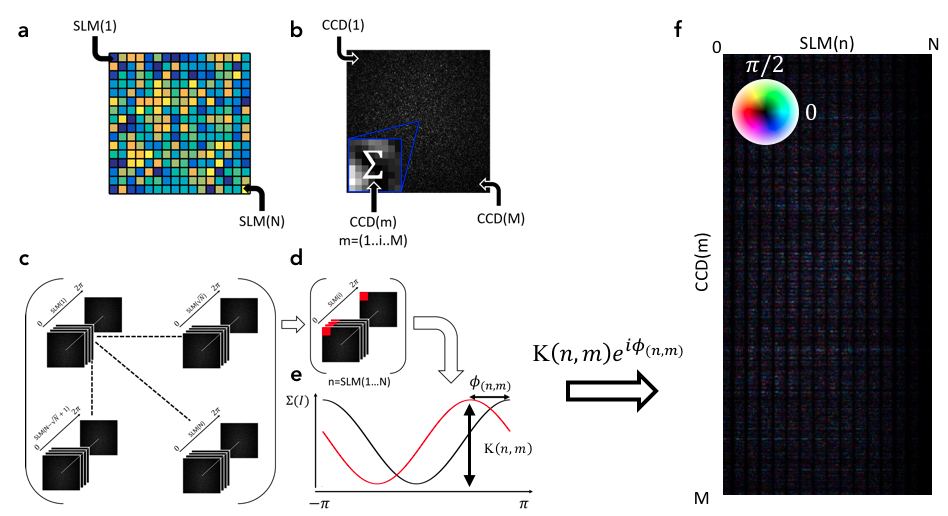
Figure 4: Process outline for the determination of the Complex Transmission Matrices.

S4 - Transmission matrices in the nonlinear regime

To model the transfer matrix in the presence of an external perturbation, it is convenient to use a Green function formalism Economou (2006); Rotter and Gigan (2017). Following this approach, the field distribution in a scattering medium can be described by $|{\bf E}\rangle={\bf K}|{\bf E}_{0}\rangle$, where ${\bf E}_{0}$ is the incident field and ${\bf K}={\bf 1}-{\bf Ge}_{s}$ is a generalized propagator, where 1 is the unitary matrix and the Green function G is such that

$$\left(\bm{\mathcal{D}}+{\bf e}\right){\bf G}={\bf 1}.$$ (1)

Here, $\bm{\mathcal{D}}({\bf r})=-\nabla\times\nabla\times$ and ${\bf e}={\bf e}_{b}+{\bf e}_{s}$ is the operator

$$\langle{\bf r}|{\bf e}|{\bf r}^{\prime}\rangle=k_{0}^{2}\varepsilon({\bf r})\delta({\bf r}-{\bf r}^{\prime})$$ (2)

associated to the relative permittivity $\varepsilon({\bf r})=\varepsilon_{b}({\bf r})+\varepsilon_{s}({\bf r})$, where $\varepsilon_{b}({\bf r})=1$ is the permittivity of the homogenous background medium and $\varepsilon_{s}({\bf r})$ is the permittivity of the scattering medium.

In position ${\bf r}$ representation the propagator can be written as

$$\langle{\bf r}|{\bf K}|{\bf r}^{\prime}\rangle={\bf 1}\delta({\bf r}-{\bf r}^{\prime})-k_{0}^{2}\varepsilon({\bf r}^{\prime})\langle{\bf r}|{\bf G}|{\bf r}^{\prime}\rangle.$$ (3)

and its matrix elements are

$$k_{mn}=\langle m|{\bf K}|n\rangle.$$ (4)

In the presence of the perturbation due to the pumping, the perturbed propagator is

$${\bf K}^{\prime}={\bf 1}-{\bf G}^{\prime}{\bf e}^{\prime}$$ (5)

with ${\bf G}^{\prime}$ the perturbed Green’s function such that

$$\left(\bm{\mathcal{D}}+{\bf e}_{b}+{\bf e}_{s}+{\bf e}^{\prime}\right){\bf G}^{\prime}={\bf 1},$$ (6)

and ${\bf e}^{\prime}$ is the operator associated to the perturbed permittivity $\Delta\varepsilon({\bf r})$, where $\varepsilon({\bf r})=\varepsilon_{b}({\bf r})+\varepsilon_{s}({\bf r})+\Delta\varepsilon({\bf r})$. The state in the presence of perturbation $|{\bf E}^{\prime}\rangle$ can then be expressed in terms of the state without perturbation $|{\bf E}\rangle$ and the input state $|{\bf E}_{0}\rangle$ as operator multiplication

$$|{\bf E}^{\prime}\rangle={\bf K}^{\prime}|{\bf E}\rangle={\bf K}^{\prime}{\bf K}|{\bf E}_{0}\rangle.$$ (7)

Correspondingly, the transmission matrix elements $k_{mn}^{\text{NL}}$ in the presence of the nonlinear perturbation can be written as a matrix multiplication

$$k_{mn}^{\text{NL}}=k^{\prime}_{mq}k_{qn}$$ (8)

where we omitted the sum over the repeated symbol $q$. By using (5), the element of the rotation matrix $k_{mq}^{\prime}$ is written as

$$k^{\prime}_{mq}=\delta_{mq}+w_{mq},$$ (9)

with $\delta_{mq}$ the Kronecker symbol and the perturbation elements

$$w_{mq}=-\langle m|{\bf G}^{\prime}{\bf e}^{\prime}|n\rangle.$$ (10)

The element of the perturbed matrix can then be written as

$$k_{mn}^{\text{NL}}=k_{mn}+w_{mq}k_{qn}=k_{mn}+w_{m1}k_{1n}+...+w_{mN}k_{Nn}.$$ (11)

Eq. (11) can be interpreted as follows: in the absence of perturbation light is channelled - with amplitude proportional to $k_{mn}$ - from the channel $n$ to the channel $m$; in the presence of the perturbation, further contributions arise from other channels. For example, the light channeled from $n$ to $1$ with amplitude $k_{1n}$ also contributes to the signal in the channel $m$ with amplitude $w_{m1}$. This may be described by stating that nonlinearity add furthers channels for light by scattering from one unperturbed channel to another.

Eq. (11) can be written following Vellekoop and Mosk (2008):

$$k_{mn}^{\text{NL}}=k_{mn}\frac{1+\xi_{mn}}{\sqrt{1+2\phi_{NL}^{2}}},=k_{mn}e^{\imath\kappa_{mn}\phi_{NL}}$$ (12)

being $\xi_{mn}$ a complex Gaussian variable with zero mean and (for small perturbations $\phi_{NL}$) $\langle|\xi_{mn}|^{2}\rangle=2\phi_{NL}^{2}$, and defining the modal dependent coefficients by

$$\kappa_{mn}\phi_{NL}=\arg(1+{\xi_{mn}})\simeq\Im({\xi_{mn}})$$ (13)

such that $\phi_{NL}$ represents the average phase shift of the mode, and $\langle|\kappa_{mn}|^{2}\rangle=1$. Additionally, as the overall transmission of the sample changes in a negligible way, the transmission matrix is such that

$$\langle|k_{mn}^{\text{NL}}|^{2}\rangle=\langle|k_{mn}|^{2}\rangle.$$ (14)

Theoretical estimate of the perturbation — To obtain a theoretical estimate of the parameter $\phi_{NL}$ we make use of eqs. (11) and (12) to show that

$$2\phi_{NL}^{2}=\langle|\xi_{mn}|^{2}\rangle=\langle|\sum_{q}\frac{w_{mq}k_{qn}}{k_{mn}}|^{2}\rangle=\langle|\sum_{q}w_{mq}|^{2}\rangle=2\langle\left[\Im\left(\sum_{q}w_{mq}\right)\right]^{2}\rangle,$$ (15)

which means that $\phi_{NL}$ represents the standard deviation of a Gaussian variable (the sum of many complex variables), which is independent of the mode indices $m$ and $n$ as is true for the average of $k_{mn}$. Therefore, the bracket in (15) can be taken as average over the modes and the disorder realizations.

From eq. (10) we have

$$\sum_{q}w_{mq}=\sum_{q}\langle m|{\bf G}^{\prime}{\bf e}^{\prime}|q\rangle\simeq\sum_{q}\langle m|{\bf G}{\bf e}^{\prime}|q\rangle$$ (16)

Where we have used ${\bf G}^{\prime}\simeq{\bf G}$ as we are interested in the lowest order approximation with respect to ${\bf e}^{\prime}$.

By using the modal representation of the Green function Economou (2006)

$${\bf G}=c^{2}\sum_{j}\frac{|j\rangle\langle j|}{\omega^{2}-\omega_{j}^{2}}\text{,}$$ (17)

where we adopt the canonical orthonormal set, gives

$$\sum_{q}w_{mq}=\sum_{q}\frac{\langle m|c^{2}{\bf e}^{\prime}|q\rangle}{\omega^{2}-\omega_{m}^{2}}=\sum_{q}\frac{\omega^{2}}{\omega^{2}-\omega_{m}^{2}}\int\Delta\varepsilon({\bf r})\bm{\phi}_{m}({\bf r})^{*}\cdot\bm{\phi}_{q}({\bf r})\,\mathrm{d}{\bf r}$$ (18)

where in the last equation we used the position representation.

A further simplification can be obtained by observing that eq. (18) is the sum of $N$ terms which all are of the order of $\int\Delta\varepsilon({\bf r})\bm{\phi}_{m}({\bf r})^{*}\cdot\bm{\phi}_{m}({\bf r})\,\mathrm{d}{\bf r}$ if $\Delta\varepsilon({\bf r})$ is a perturbation that involves most of the sample and couples all the modes, and if the modes are not strongly localized. In this approximation we can write

$$\sum_{q}w_{mq}\simeq N\frac{\omega^{2}}{\omega^{2}-\omega_{m}^{2}}\int\Delta\varepsilon({\bf r})\bm{\phi}_{m}({\bf r})^{*}\cdot\bm{\phi}_{m}({\bf r})\,\mathrm{d}{\bf r}$$ (19)

We recall one can write

$$\frac{1}{\omega^{2}-\omega_{m}^{2}}=PV\left[\frac{1}{\omega^{2}-\omega_{m}^{2}}\right]+\frac{\imath\pi}{2\omega}\delta(\omega-\omega_{m})$$ (20)

with $PV$ the principal value. As $\xi_{mn}$ is the sum of many random contributions, the real and the imaginary part will be Gaussian variables with the same variance.

Averaging (19) over all the modes (the average quantities are expected to be modal independent), by summing w.r.t. to the index $m$ and dividing by $N$ we have

$$\Im\left(\sum_{q}w_{mq}\right)\simeq\frac{\pi\omega}{2}\int\Delta\varepsilon({\bf r})\rho({\bf r},\omega)\,\mathrm{d}{\bf r}$$ (21)

where we used the expression for the LDOS

$$\rho({\bf r},\omega)=\sum_{m}\delta(\omega-\omega_{m})\bm{\phi}_{m}({\bf r})^{*}\cdot\bm{\phi}_{m}({\bf r})$$ (22)

Finally we have

$$\phi_{NL}^{2}=\frac{1}{2}\langle|\sum w_{mq}|^{2}\rangle=\langle\left[\Im\left(\sum_{q}w_{mq}\right)\right]^{2}\rangle\simeq\frac{\pi^{2}\omega^{2}}{4}\langle\left(\int\Delta\varepsilon({\bf r})\rho({\bf r},\omega)\,\mathrm{d}{\bf r}\right)^{2}\rangle.$$ (23)

References

• Popoff et al. (2010) S. Popoff, G. Lerosey, R. Carminati, M. Fink, A. C. Boccara,  and S. Gigan, Physical Review Letters 104, 100601 (2010).
• Van de Hulst (1981) H. C. Van de Hulst, Light scattering by small particles (Dover Publications, Inc., 1981).
• Economou (2006) E. E. Economou, Green’s Functions in Quantum Physics (Springer, 2006).
• Rotter and Gigan (2017) S. Rotter and S. Gigan, Reviews of Modern Physics 89, 015005 (2017).
• Vellekoop and Mosk (2008) I. M. Vellekoop and A. Mosk, Optics Communications 281, 3071 (2008).