Effect of external magnetic field on nucleon mass in hot and dense medium : Inverse Magnetic Catalysis in Walecka Model

Abstract

Vacuum to nuclear matter phase transition has been studied in presence of constant external background magnetic field with the mean field approximation in Walecka model. The anomalous nucleon magnetic moment has been taken into account using the modified “weak” field expansion of the fermion propagator having non-trivial correction terms for charged as well as for neutral particles. The effect of nucleon magnetic moment is found to favour the magnetic catalysis effect at zero temperature and zero baryon density. However, extending the study to finite temperatures, it is observed that the anomalous nuclear magnetic moment plays a crucial role in characterizing the qualitative behaviour of vacuum to nuclear matter phase transition even in case of the weak external magnetic fields . The critical temperature corresponding to the vacuum to nuclear medium phase transition is observed to decrease with the external magnetic field which can be identified as the inverse magnetic catalysis in Walecka model whereas the opposite behaviour is obtained in case of vanishing magnetic moment indicating magnetic catalysis.

I Introduction

Understanding Quantum Chromodynamics (QCD) in presence of magnetic background has gained lots of contemporary research interests ln871 . It is important to study QCD in presence of external magnetic field not only for its relevance with the astrophysical phenomena prep442 ; prl95 ; prd76 ; prl100 ; prdN76 ; prl105 ; prd82 but also due to the possibility of strong magnetic field generation in non-central heavy-ion collision ijmp which sets the stage for investigation of this magnetic modifications. Although the background fields produced in RHIC and LHC are much smaller in comparison with the field strengths prevailed during the cosmological electro-weak phase transition which may reach up to $eB\approx 200m_{\pi}^{2}$ plb265 , they are strong enough to cast significant influence on the hadronic properties which bear the information of the chiral phase transition. At vanishing chemical potential, modification due to the presence of magnetic background can be obtained from first principle using lattice QCD simulations prd82M ; prd83 which shows monotonic increase in critical temperature with the increasing magnetic field. The effects of external magnetic field on the chiral phase transition has been studied using different effective models in recent years prd81 ; prd84 ; prc83 ; prd83M ; prc83A ; prd82R ; prd83K ; prd85 ; jhep08 ; prd82A ; prd85S ; prd84D ; prd86E . QCD being a confining theory at low energies, effective theories are employed to describe the low energy behaviour of the strong interaction. In such a theory, the condensate is described as the non-zero expectation value of the sigma field which is basically a composite operator of two quark fields. If the condensate is already present without any background field, the effect of its enhancement in presence of the external magnetic field is described as magnetic catalysis(MC). Effective field theoretic models in general contain a few parameters which can be fixed from experimental inputs. Although most of the model calculations are in support of MC, some lattice results had shown inverse magnetic catalysis(IMC) where critical temperature follows the opposite trend jhep1202 ; prdB86 ; jhep04 ; prd90 . It was pointed out in jhep1304 that IMC is attributed to the dominance of the sea contribution over the valence contribution of the quark condensate. The sea effect has not been incorporated even in the Polyakov loop extended versions of Nambu–Jona-Lasinio (PNJL) model and Quark-Meson(PQM) model which might be a possible reason for the disagreement. To investigate the apparent contradiction, a significant amount of work has been done rmp88 in quest of proper modifications of the effective models, most of which are focused on the magnetic field dependence of the coupling constants or other magnetic field dependent parameters in the model. Very recently, IMC has been observed in NJL model, with Pauli-Villars regularization scheme plb758 which gives markedly different behaviour in comparison with the usual soft-cutoff approach.

In the context of nuclear physics, the MC effect was discussed by Haber et al in Ref.Haber:2014ula . There, the effect of background magnetic field on the transition between vacuum to nuclear matter at zero temperature was studied for the Walecka model walecka1 as well as for the extended linear sigma model. The study includes the B-dependent Dirac sea contribution of the free energy density which was ignored previously (see for example haber32 ; haber33 ; haber34 ; haber35 ; haber36 ; haber37 ; haber38 ; haber39 ; haber40 ) in the case of magnetized nuclear matter. Following the renormalization procedure similar to the case of magnetized quark matter, the cut-off dependence of the B-dependent sea contribution is absorbed into a renormalized magnetic field and a renormalized electric charge. The onset of the vacuum to nuclear matter phase transition is determined by equating the corresponding free energies. From the qualitative agreement between the two models, it is evident that with the proper incorporation of the magnetic catalysis effect, the creation of the nuclear matter becomes energetically more expensive in presence of the background magnetic field. However, there exist an important qualitative difference between the two models. As the analysis suggests, only in case of the Walecka model, there exists a region where the critical chemical potential for the vacuum to nuclear matter transition is lower than the same in the absence of the background field. This feature has surprising similarities with the inverse magnetic catalysis(IMC) shown in NJL and holographic Sakai-Sugimoto model haber15 . It is interesting to see whether similar feature exists also in a more generalized scenario. Now, as the anomalous magnetic moment(AMM) of the nucleons has not been taken into account in the analysis, an obvious generalization will be to incorporate it in the study of vacuum to nuclear matter phase transition under external magnetic field at non-zero temperature. A recent study referee incorporating the magnetic field dependent vacuum in presence of finite temperature and density, however, shows that the AMM of charged fermions makes no significant contribution to the equation of state at any external field value. Thus, among others, it will be interesting to see whether MC persists in the presence of anomalous magnetic moment.

In this work we restrict ourselves only in the “weak” field regime of the external magnetic field and use the Walecka model to describe the nucleon-nucleon interaction. In this model, the interaction between the nucleons are described by the exchange of scalar ($\sigma$) and vector($\omega$) mesons. More realistic extension of the Walecka model where the self-interactions of the meson fields are also considered is ignored here for the sake of simplicity as they hardly contribute to the qualitative nature of the results presented in this work. Now, to obtain the effective mass of the nucleons, instead of minimizing the free energy density with respect to the condensate Haber:2014ula , we calculate the effective nucleon propagator by summing up the scalar and vector tadpole diagrams self-consistently. In that case, the effective mass of the nucleon appears as a pole of the effective nucleon propagator. In case of weak magnetic field, the nucleon propagators can be expressed as a series in powers of $qB$ and $\kappa B$ where $q$ and $\kappa$ represents the charge and the anomalous magnetic moment of the nucleons. It should be mentioned here that in the calculation of the tadpole diagrams using the interacting propagator, we employ mean field approximation. It is essentially equivalent to solving the meson field equations with the replacement of the meson field operators by their expectation values. In other words, under this approximation, the meson field operators are rendered into classical fields assumed to be uniform in space and time and the fluctuation around this background is neglected.

The article is organized as follows. In Sec. II, the familiar expression ayala_scalar of the weak field expansion of the charged scalar propagator in presence of the constant external magnetic field is derived using the perturbative method. The same procedure is employed in Sec. III to obtain the weak field expanded propagators of the charged and neutral fermion with non-zero magnetic moment. The suitable form of the corresponding thermal propagators are also discussed which are used to obtain the effective mass of the nucleons in case of Walecka model described in Sec. IV. Sec. V contains the numerical results and discussions. Finally, we summarize our work in Sec. VI.

II charged scalar propagator under external magnetic field

Let us first consider the propagation of a charged scalar particle under zero external magnetic field. In this case, the scalar vacuum Feynman propagator $\Delta_{F}\left(x,x^{\prime}\right)=\Delta_{F}\left(x-x^{\prime}\right)$ satisfies

$$\left(\partial_{\mu}\partial^{\mu}+m^{2}\right)\Delta_{F}\left(x-x^{\prime}\right)=\delta^{4}\left(x-x^{\prime}\right)~{}.$$ (1)

In order to solve Eq. (1), we introduce the Fourier transform of $\Delta_{F}\left(x-x^{\prime}\right)$ by

$$\Delta_{F}\left(x-x^{\prime}\right)=\int\frac{d^{4}k}{\left(2\pi\right)^{4}}e^{-ik\cdot\left(x-x^{\prime}\right)}\Delta_{F}\left(k\right)~{},$$ (2)

where, $\Delta_{F}\left(k\right)$ is the momentum space vacuum scalar propagator. Substituting $\Delta_{F}\left(x-x^{\prime}\right)$ from Eq. (2) into Eq. (1), we get

$$\Delta_{F}\left(k\right)=\left(\frac{-1}{k^{2}-m^{2}+i\epsilon}\right)~{},$$ (3)

where we have imposed the Feynman’s boundary condition and put the $i\epsilon$ in the denominator.

We now turn on the external magnetic field. In this case, the charged scalar propagator under external magnetic field, denoted by $\Delta_{B}\left(x,x^{\prime}\right)$ will satisfy,

$$\left[\left\{\frac{}{}\partial_{\mu}+iqA_{\mu}\left(x\right)\right\}\left\{\frac{}{}\partial^{\mu}+iqA^{\mu}\left(x\right)\right\}+m^{2}\right]\Delta_{B}\left(x,x^{\prime}\right)=\delta^{4}\left(x-x^{\prime}\right)~{},$$ (4)

where, $q$ is the electric charge of the particle and $A^{\mu}\left(x\right)$ is the four potential corresponding to the external magnetic field. It is to be noted that, the propagator $\Delta_{B}\left(x,x^{\prime}\right)$ is not translational invariant. For solving Eq. (4), we follow the procedure as given in Ref Nieves:2004qp ; Nieves:2006xp and choose a particular gauge in which the four potential is

$$A^{\mu}\left(x\right)=-\frac{1}{2}F^{\mu\nu}x_{\nu}~{}.$$ (5)

For the case of a constant external magnetic field, the field strength tensor $F^{\mu\nu}$ is independent of $x$. Substituting Eq. (5) into Eq. (4), we get

$$\left[\Box+m^{2}-iqF^{\mu\nu}x_{\nu}\partial_{\mu}-\frac{q^{2}}{4}F^{\mu\alpha}F_{\mu\beta}x_{\alpha}x^{\beta}\right]\Delta_{B}\left(x,x^{\prime}\right)=\delta^{4}\left(x-x^{\prime}\right)~{}.$$ (6)

The corresponding momentum space propagator $\Delta_{B}\left(k\right)$ is obtained from the Fourier transform of the translational invariant part of the coordinate space propagator $\Delta_{B}\left(x,x^{\prime}\right)$ i.e.

$$\Delta_{B}\left(x,x^{\prime}\right)=\phi\left(x,x^{\prime}\right)\int\frac{d^{4}k}{\left(2\pi\right)^{4}}e^{-ik\cdot\left(x-x^{\prime}\right)}\Delta_{B}\left(k\right)~{},$$ (7)

where, $\phi\left(x,x^{\prime}\right)$ is the phase factor and it depends on the choice of gauge. For the gauge given in Eq. (5), the phase factor comes out to be Nieves:2006xp ,

$$\phi\left(x,x^{\prime}\right)=\exp\left[\frac{i}{2}qF^{\alpha\beta}x_{\alpha}x^{\prime\beta}\right]~{}.$$ (8)

Substituting Eq. (7) into Eq. (6), we get

$$\int\frac{d^{4}k}{\left(2\pi\right)^{4}}e^{-ik\cdot\left(x-x^{\prime}\right)}\Delta_{B}\left(k\right)\left[\Box+m^{2}-2ik_{\mu}\partial^{\mu}-k^{2}-qF^{\mu\nu}x_{\nu}k_{\mu}-\frac{1}{4}q^{2}F^{\mu\alpha}F_{\mu\beta}x_{\alpha}x^{\beta}\right]\phi\left(x,x^{\prime}\right)=\delta^{4}\left(x-x^{\prime}\right)~{}.$$ (9)

We further substitute $\phi\left(x,x^{\prime}\right)$ from Eq. (8) into Eq. (9) and obtain

$$\int\frac{d^{4}k}{\left(2\pi\right)^{4}}e^{-ik\cdot\left(x-x^{\prime}\right)}\Delta_{B}\left(k\right)\left[-k^{2}+m^{2}-qk^{\mu}F_{\mu\nu}\left(x-x^{\prime}\right)^{\nu}-\frac{1}{4}q^{2}F^{\mu\alpha}F_{\mu\beta}\left(x-x^{\prime}\right)_{\alpha}\left(x-x^{\prime}\right)^{\beta}\right]=\delta^{4}\left(x-x^{\prime}\right)~{},$$ (10)

where we have used the fact that $\phi\left(x,x\right)=1$. This can be verified from Eq. (8) using the antisymmetric property of $F^{\mu\nu}$. Each term in Eq. (10) is now translationally invariant and can be expressed as,

$$\int\frac{d^{4}k}{\left(2\pi\right)^{4}}\Delta_{B}\left(k\right)\left[-k^{2}+m^{2}-iqk^{\mu}F_{\mu\nu}\tilde{\partial}^{\nu}+\frac{1}{4}q^{2}F^{\mu\alpha}F_{\mu\beta}\tilde{\partial}_{\alpha}\tilde{\partial}^{\beta}\right]e^{-ik\cdot\left(x-x^{\prime}\right)}=\delta^{4}\left(x-x^{\prime}\right)~{},$$ (11)

where we have used the notation $\tilde{\partial}_{\mu}=\left(\frac{\partial}{\partial k^{\mu}}\right)$. In order to extract $\Delta_{B}\left(k\right)$ from Eq. (11), it is necessary to swap the positions of $\Delta_{B}\left(k\right)$ and $e^{-ik\cdot\left(x-x^{\prime}\right)}$. This swapping is done at the cost of addition of a term, which contains a total four momentum derivative ($\tilde{\partial}_{\mu}J^{\mu}$) i.e.

$$\int\frac{d^{4}k}{\left(2\pi\right)^{4}}e^{-ik\cdot\left(x-x^{\prime}\right)}\left[-k^{2}+m^{2}+iqF_{\mu\nu}\tilde{\partial}^{\nu}k^{\mu}+\frac{1}{4}q^{2}F^{\mu\alpha}F_{\mu\beta}\tilde{\partial}_{\alpha}\tilde{\partial}^{\beta}\right]\Delta_{B}\left(k\right)+\int\frac{d^{4}k}{\left(2\pi\right)^{4}}\tilde{\partial}_{\mu}J^{\mu}=\delta^{4}\left(x-x^{\prime}\right)~{}.$$ (12)

$J^{\mu}$ in the above equation contains the propagator $\Delta_{B}\left(k\right)$. Now the $d^{4}k$ integral of second term on the L.H.S. can be converted to a surface integral using Gauss’s theorem and assuming $D\left(k\right)$ to be well behaved function, this term will vanish. So the momentum space propagator $\Delta_{B}\left(k\right)$ satisfies the following differential equation,

$$\left[-k^{2}+m^{2}+iqF_{\mu\nu}\tilde{\partial}^{\nu}k^{\mu}+\frac{1}{4}q^{2}F^{\mu\alpha}F_{\mu\beta}\tilde{\partial}_{\alpha}\tilde{\partial}^{\beta}\right]\Delta_{B}\left(k\right)=1$$ (13)

Let us now consider a constant external magnetic field in the +ve z-direction i.e. $\vec{B}=B\hat{z}$, which implies that the non-zero components of the electromagnetic field strength tensor $F^{\mu\nu}$ are $F^{12}=-F^{21}$. So any four vector $a^{\mu}\equiv\left(a^{0},a^{1},a^{2},a^{3}\right)$ is decomposed into $a^{\mu}=\left(a_{\parallel}^{\mu}+a_{\perp}^{\mu}\right)$ with $a^{\mu}_{\parallel}\equiv\left(a^{0},0,0,a^{3}\right)$ and $a^{\mu}_{\perp}\equiv\left(0,a^{1},a^{2},0\right)$. The corresponding metric tensors are $g_{\parallel}^{\mu\nu}=diag\left(1,0,0,-1\right)$ and $g_{\perp}^{\mu\nu}=diag\left(0,-1,-1,0\right)$ satisfying $g^{\mu\nu}=\left(g_{\parallel}^{\mu\nu}+g_{\perp}^{\mu\nu}\right)$. Therefore the propagator $\Delta_{B}\left(k\right)$ being a Lorentz scalar, will be functions of $k_{\parallel}^{2}$ and $k_{\perp}^{2}$ i.e. $\Delta_{B}\left(k\right)=\Delta_{B}\left(k_{\parallel}^{2},k_{\perp}^{2}\right)$. Hence the third term within the square bracket in the L.H.S. of Eq. (13) can be written as,

$$iqF_{\mu\nu}\tilde{\partial}^{\nu}\left[k^{\mu}\Delta_{B}\left(k_{\parallel}^{2},k_{\perp}^{2}\right)\right]=iqF_{\mu\nu}\left[g^{\mu\nu}+2k^{\mu}k_{\parallel}^{\nu}\frac{\partial}{\partial k_{\parallel}^{2}}+2k^{\mu}k_{\perp}^{\nu}\frac{\partial}{\partial k_{\perp}^{2}}\right]\Delta_{B}\left(k_{\parallel}^{2},k_{\perp}^{2}\right)=0~{}.$$ (14)

It is also trivial to check that

$$F^{\mu\alpha}F_{\mu\beta}\tilde{\partial}_{\alpha}\tilde{\partial}^{\beta}=B^{2}g_{\perp}^{\alpha\beta}\tilde{\partial}_{\alpha}\tilde{\partial}_{\beta}=B^{2}\tilde{\Box}_{\perp}~{},$$ (15)

where, $\tilde{\Box}_{\perp}=g_{\perp}^{\mu\nu}\tilde{\partial}_{\alpha}\tilde{\partial}_{\beta}$. Finally Eq. (13) becomes,

$$\left[-k^{2}+m^{2}+\frac{1}{4}\left(qB\right)^{2}\tilde{\Box}_{\perp}\right]\Delta_{B}\left(k\right)=1~{}.$$ (16)

We now expand the propagator as a power series in $qB$,

$$\Delta_{B}\left(k\right)=\sum_{i=0}^{\infty}\left(qB\right)^{i}\Delta_{i}\left(k\right)$$ (17)

and substitute in Eq. (16) to obtain,

$$\sum_{i=0}^{\infty}\left[\left(qB\right)^{i}\left(-k^{2}+m^{2}\right)+\left(qB\right)^{i+2}\frac{1}{4}\tilde{\Box}_{\perp}\right]\Delta_{i}\left(k\right)=1~{}.$$ (18)

Equating the coefficients of different powers of $qB$ in the both side of the above equation, we get,

$$\Delta_{0}\left(k\right) = \left(\frac{-1}{k^{2}-m^{2}+i\epsilon}\right)$$

$$\Delta_{1}\left(k\right) = 0$$

$$\Delta_{n}\left(k\right) = -\Delta_{0}\left(k\right)\frac{1}{4}\tilde{\Box}_{\perp}\Delta_{n-2}\left(k\right)~{}~{}\text{for}~{}~{}n\geq 2~{}.$$ (19)

Eq. (19) is a recursion relation and it immediately follows that $\Delta_{3}\left(k\right)=\Delta_{5}\left(k\right)=\Delta_{7}\left(k\right)=.....=0$. Using this relation one can calculate the charged scalar propagator up to any order in $eB$. As for example,

$$\Delta_{2}\left(k\right)=-\Delta_{0}\left(k\right)\frac{1}{4}\tilde{\Box}_{\perp}\Delta_{0}\left(k\right)=\left[\frac{k_{\parallel}^{2}-k_{\perp}^{2}-m^{2}}{\left(k^{2}-m^{2}+i\epsilon\right)^{4}}\right]~{}.$$

Therefore the propagator becomes,

$$\Delta_{B}\left(k\right) = \Delta_{0}\left(k\right)+\left(qB\right)^{2}\Delta_{2}\left(k\right)+\mathcal{O}\left(qB\right)^{4}$$ (20)

$$= \left(\frac{-1}{k^{2}-m^{2}+i\epsilon}\right)+\left(qB\right)^{2}\left[\frac{k_{\parallel}^{2}-k_{\perp}^{2}-m^{2}}{\left(k^{2}-m^{2}+i\epsilon\right)^{4}}\right]+\mathcal{O}\left(qB\right)^{4}~{}.$$

III fermion propagator under external magnetic field

Following the similar procedure described in the previous section, we find that the Dirac equation with anomalous magnetic moment ($\kappa$) in the momentum space representation is given by Nieves:2004qp ; Nieves:2006xp

$$\Big{[}p\!\!\!/-\frac{i}{2}qF^{\mu\nu}\gamma_{\mu}\frac{\partial}{\partial p^{\nu}}-m_{f}-\frac{1}{2}\kappa\sigma\cdot F\Big{]}S_{B}(p)=1.$$ (21)

The strategy to obtain the power expansion is to write

$$S_{B} = S_{0}+S_{1}.$$ (22)

where $S_{0}$ represents the vacuum propagator and $S_{1}$ represents its linear order correction in presence of external magnetic field. Now, let us define the operator

$$\hat{O} = \Big{[}\frac{i}{2}qF^{\mu\nu}\gamma_{\mu}\frac{\partial}{\partial p^{\nu}}+\frac{1}{2}\kappa\sigma\cdot F\Big{]}$$ (23)

Using the perturbative expansion in the Dirac equation and neglecting the higher order $\hat{O}S_{1}$ term one obtains

$$S_{1} = S_{0}\hat{O}S_{0}.$$ (24)

Thus the linear order correction to the weak expansion of the propagator is nothing but an operator of non-commutative gamma matrices and differentials sandwiched between the familiar vacuum propagators. Following the similar strategy one can extend the series to higher order terms in powers of $B$. As we shall see that in our case, the leading order contribution of the external magnetic field occurs due to the quadratic correction of the weak field propagator and not due to the simpler linear order one, we must extend the perturbative series as

$$S_{B} = S_{0}+S_{1}+S_{2}$$ (25)

for which one obtains

$$S_{2} = S_{0}\hat{O}S_{1}$$ (26)

where $S_{1}=S_{0}\hat{O}S_{0}$ is given by ( see Nieves:2004qp ; Nieves:2006xp )

$$S_{1} = \frac{1}{(p^{2}-m_{f}^{2}+i\epsilon)^{2}}$$ (27)

$$\times \Big{[}qB\gamma_{5}\big{[}(p\cdot b)u\!\!\!/-(p\cdot u)b\!\!\!/+m_{f}u\!\!\!/b\!\!\!/\big{]}+\kappa B\big{[}(p\!\!\!/+m_{f})\gamma_{5}u\!\!\!/b\!\!\!/(p\!\!\!/+m_{f})\big{]}\Big{]}$$

with $u^{\mu}\equiv(1,0,0,0)$ and $b^{\mu}\equiv(0,0,0,1)$ in the fluid rest frame. It is straightforward to derive the expression of $S_{2}$ and after plugging the correction terms we finally obtain the weak field expansion of the fermion propagator given by

$$S_{B}\left(p,m\right) = \frac{-\left(\cancel{p}+m\right)}{p^{2}-m^{2}+i\epsilon}+\left(qB\right)\frac{i\gamma^{1}\gamma^{2}\left(\cancel{p}_{\parallel}+m\right)}{\left(p^{2}-m^{2}+i\epsilon\right)^{2}}+\left(\kappa B\right)\frac{\left(\cancel{p}+m\right)i\gamma^{1}\gamma^{2}\left(\cancel{p}+m\right)}{\left(p^{2}-m^{2}+i\epsilon\right)^{2}}$$ (28)

$$+\left(qB\right)^{2}\frac{-2\left\{p_{\perp}^{2}\left(\cancel{p}_{\parallel}+m\right)-\cancel{p}_{\perp}\left(p_{\parallel}^{2}-m^{2}\right)\right\}}{\left(p^{2}-m^{2}+i\epsilon\right)^{4}}+\left(qB\right)\left(\kappa B\right)\frac{-4\cancel{p}_{\parallel}\left(\cancel{p}_{\parallel}+m\right)+p^{2}-m^{2}}{\left(p^{2}-m^{2}+i\epsilon\right)^{3}}$$

$$+\left(\kappa B\right)^{2}\frac{-\left(\cancel{p}+m\right)\left(\cancel{p}_{\parallel}-\cancel{p}_{\perp}+m\right)\left(\cancel{p}+m\right)}{\left(p^{2}-m^{2}+i\epsilon\right)^{3}}+\mathcal{O}\left(B^{3}\right)~{}.$$

In order to express $S_{B}\left(p,m\right)$ in a more compact form, we use the procedure given in Ref. Bandyopadhyay:2017raf and write

$$\left(\frac{-1}{p^{2}-m^{2}+i\epsilon}\right)^{n}=\left.\hat{A}_{n-1}\Delta_{F}\left(p,m_{1}\right)\right|_{m_{1}=m}$$ (29)

where,

$$\Delta_{F}\left(p,m\right)=\left(\frac{-1}{p^{2}-m^{2}+i\epsilon}\right)$$ (30)

and

$$\hat{A}_{n}=\frac{\left(-1\right)^{n}}{n!}\frac{\partial^{n}}{\partial\left(m_{1}^{2}\right)^{n}}~{}.$$ (31)

Using Eqs. (29)-(31), we can rewrite Eq. (28) as

$$S_{B}\left(p,m\right)=\left.\hat{F}\left(p,m,m_{1}\right)\Delta_{F}\left(p,m_{1}\right)\right|_{m_{1}=m}$$ (32)

where,

$$\hat{F}\left(p,m,m_{1}\right) = \left(\cancel{p}+m\right)+\left(qB\right)i\gamma^{1}\gamma^{2}\left(\cancel{p}_{\parallel}+m\right)\hat{A}_{1}+\left(\kappa B\right)\left(\cancel{p}+m\right)i\gamma^{1}\gamma^{2}\left(\cancel{p}+m\right)\hat{A}_{1}$$ (33)

$$-2\left(qB\right)^{2}\left\{p_{\perp}^{2}\left(\cancel{p}_{\parallel}+m\right)-\cancel{p}_{\perp}\left(p_{\parallel}^{2}-m^{2}\right)\right\}\hat{A}_{3}+\left(qB\right)\left(\kappa B\right)\left\{4\cancel{p}_{\parallel}\left(\cancel{p}_{\parallel}+m\right)-p^{2}+m^{2}\right\}\hat{A}_{2}$$

$$+\left(\kappa B\right)^{2}\left(\cancel{p}+m\right)\left(\cancel{p}_{\parallel}-\cancel{p}_{\perp}+m\right)\left(\cancel{p}+m\right)\hat{A}_{2}+\mathcal{O}\left(B^{3}\right)~{}.$$

We conclude this section by mentioning the fermion propagator at finite temperature and density along with external magnetic field. For this, we use the real time formalism of thermal field theory where the thermal propagator becomes $2\times 2$ matrix. However, it is sufficient to know the $11$-component of the matrix propagator Mallik:2016anp which is given by DOlivo:2002omk ,

$$S_{11}\left(p,m\right)=S_{B}\left(p\right)-\eta\left(p\cdot u\right)\left[S_{B}\left(p\right)-\gamma^{0}S_{B}^{\dagger}\left(p\right)\gamma^{0}\right]$$ (34)

where,

$$\eta\left(p\cdot u\right)=\Theta\left(p\cdot u\right)f_{+}\left(p\cdot u\right)+\Theta\left(-p\cdot u\right)f_{-}\left(-p\cdot u\right)$$ (35)

with

$$f_{\pm}\left(p\cdot u\right)=\left[\exp\left(\frac{p\cdot u\mp\mu}{T}\right)+1\right]^{-1}~{}.$$ (36)

Substituting Eq. (32) into Eq. (34) and using the fact that $\gamma^{0}\hat{F}^{\dagger}\left(p,m,m_{1}\right)\gamma^{0}=\hat{F}\left(p,m,m_{1}\right)$, we get

$$S_{11}\left(p,m\right)=\left.\hat{F}\left(p,m,m_{1}\right)\left[\frac{}{}\Delta_{F}\left(p,m_{1}\right)-2\pi i\eta\left(p\cdot u\right)\delta\left(p^{2}-m_{1}^{2}\right)\right]\right|_{m_{1}=m}$$ (37)

IV Effective mass of nucleon in Walecka model

The propagation of nucleons in hot and dense nuclear matter is well described using Quantum Hadrodynamics (QHD) details of which can be found in Ref. Negele:1986bp ; Alam:1999sc . We briefly summarize the main the formalism of QHD at zero magnetic field. We start with the real time thermal propagator matrix of the nucleon  Mallik:2016anp ; bellac ,

$$\bm{S}_{0}\left(p,m_{N}\right)=\left(\cancel{p}+m_{N}\right)\bm{V}\left[\begin{array}[]{cc}\Delta_{F}\left(p,m_{N}\right)&0\\ 0&-\Delta_{F}^{*}\left(p,m_{N}\right)\end{array}\right]\bm{V}$$ (40)

where the diagonalizing matrix $\bm{V}$ is given by,

$$\bm{V}=\left[\begin{array}[]{cc}N_{2}&-N_{1}e^{\beta\mu/2}\\ N_{1}e^{-\beta\mu/2}&N_{2}\end{array}\right]$$ (43)

with

$$N_{1}\left(p\cdot u\right) = \sqrt{f_{+}\left(p\cdot u\right)}\Theta\left(p\cdot u\right)+\sqrt{f_{-}\left(-p\cdot u\right)}\Theta\left(-p\cdot u\right)$$

$$N_{2}\left(p\cdot u\right) = \sqrt{1-f_{+}\left(p\cdot u\right)}\Theta\left(p\cdot u\right)+\sqrt{1-f_{-}\left(-p\cdot u\right)}\Theta\left(-p\cdot u\right)~{}.$$

In Walecka model, the nucleons interact with the scalar meson $\sigma$ and vector meson $\omega$. The interaction Lagrangian is

$$\mathscr{L}_{QHD}=g_{\sigma NN}\bar{\Psi}\Psi\sigma-g_{\omega NN}\bar{\Psi}\gamma^{\mu}\Psi\omega_{\mu}~{},$$ (44)

where $\Psi=\left[\begin{array}[]{c}p\\ n\end{array}\right]$ is the nucleon isospin doublet and the value of the coupling constants are given by $g_{\sigma NN}=9.57$ and $g_{\omega NN}=11.67$ Negele:1986bp . The complete nucleon propagator matrix $\bm{S^{\prime}}\left(p,m_{N}\right)$ in presence of these interactions is obtained from the Dyson-Schwinger equation given by,

$$\bm{S^{\prime}}=\bm{S}_{0}-\bm{S}_{0}\bm{\Sigma}\bm{S^{\prime}}$$ (45)

where, $\bm{\Sigma}$ is the one-loop thermal self energy matrix of the nucleon. It can be shown that Mallik:2016anp , the complete propagator and the self energy matrices are diagonalized by $\bm{V}$ and $\bm{V}^{-1}$ respectively. This in turn diagonalizes the Dyson-Schwinger equation and Eq. (45) becomes an algebraic equation (in thermal space),

$$\overline{S^{\prime}}=\overline{S}_{0}-\overline{S}_{0}\overline{\Sigma}~{}\overline{S^{\prime}}~{}.$$ (46)

It is to be noted that, each term in the above equation is $4\times 4$ matrix in Dirac space. Here $\overline{S}_{0}\left(p,m_{N}\right)=-\left(\cancel{p}+m_{N}\right)\Delta_{F}\left(p,m_{N}\right)$ and $\overline{\Sigma}$ is the $11$-component of the matrix $\bm{V}^{-1}\bm{\Sigma}\bm{V}^{-1}$ and is called the thermal self energy function. In Walecka model the Dirac structure of $\overline{\Sigma}$ comes out to be,

$$\overline{\Sigma}=\left(\Sigma_{s}\mathds{1}+\Sigma_{v}^{\mu}\gamma_{\mu}\right)=\left(\Sigma_{s}\mathds{1}+\cancel{\Sigma}_{v}\right)~{}.$$ (47)

Using Eq. (47), we can solve Eq. (46) and obtain

$$\overline{S^{\prime}}\left(p,m_{N}\right)=\left(\cancel{P}+m_{N}^{*}\right)\Delta_{F}\left(P,m_{N}^{*}\right)$$ (48)

where

$$P=\left(p-\Sigma_{v}\right)~{}~{}~{}~{}\text{and}~{}~{}~{}~{}~{}m_{N}^{*}=\left(m+\Sigma_{s}\right)~{}.$$ (49)

We can finally write down the complete propagator matrix

$$\bm{S^{\prime}}\left(p,m_{N}\right)=\left(\cancel{P}+m_{N}^{*}\right)\bm{V}\left[\begin{array}[]{cc}\Delta_{F}\left(P,m_{N}^{*}\right)&0\\ 0&-\Delta_{F}^{*}\left(P,m_{N}^{*}\right)\end{array}\right]\bm{V}~{},$$ (52)

whose $11$-component is,

$$S^{\prime}_{11}\left(p,m_{N}\right)=S_{F}\left(P,m_{N}^{*}\right)-\eta\left(P\cdot u\right)\left[S_{F}\left(P,m_{N}^{*}\right)-\gamma^{0}S_{F}^{\dagger}\left(P,m_{N}^{*}\right)\gamma^{0}\right]~{}.$$ (53)

Figure 1: Feynman diagrams for the one-loop self energy of nucleon in Walecka model. Bold line indicates the complete/dressed propagator

Let us now calculate, the nucleon self energy function $\bar{\Sigma}$ using the interaction Lagrangian given in Eq. (44) and consider only the tadpole Feynman diagrams as shown in Fig. 1. It is to be noted that, the loop particles are dressed i.e. the propagator for the loop particles is $\bm{S^{\prime}}\left(p,m_{N}\right)$ as given in Eq. (52). Applying Feynman rule to Fig. 1 we obtain the $11$-component of the thermal self energy as,

$$\Sigma_{11} = -\left(\frac{g^{2}_{\sigma NN}}{m_{\sigma}^{2}}\right)i\int\frac{d^{4}p}{\left(2\pi\right)^{4}}\text{Tr}\left[S^{\prime~{}(\text{p})}_{11}\left(p,m_{N}\right)+S^{\prime~{}(\text{n})}_{11}\left(p,m_{N}\right)\right]$$ (54)

$$+\gamma_{\mu}\left(\frac{g^{2}_{\omega NN}}{m_{\omega}^{2}}\right)i\int\frac{d^{4}p}{\left(2\pi\right)^{4}}\text{Tr}\left[\gamma^{\mu}S^{\prime~{}(\text{p})}_{11}\left(p,m_{N}\right)+\gamma^{\mu}S^{\prime~{}(\text{n})}_{11}\left(p,m_{N}\right)\right]$$

where (p) and (n) in the superscript corresponds to proton and neutron respectively. It is easy to show that $\text{Re}\Sigma_{11}=\text{Re}\overline{\Sigma}$. So we get from Eq. (47),

$$\text{Re}\Sigma_{s} = -\left(\frac{g^{2}_{\sigma NN}}{m_{\sigma}^{2}}\right)\text{Re}~{}i\int\frac{d^{4}p}{\left(2\pi\right)^{4}}\text{Tr}\left[S^{\prime~{}(\text{p})}_{11}\left(p,m_{N}\right)+S^{\prime~{}(\text{n})}_{11}\left(p,m_{N}\right)\right]$$ (55)

$$\text{Re}\Sigma_{v}^{\mu} = \left(\frac{g^{2}_{\omega NN}}{m_{\omega}^{2}}\right)\text{Re}~{}i\int\frac{d^{4}p}{\left(2\pi\right)^{4}}\text{Tr}\left[\gamma^{\mu}S^{\prime~{}(\text{p})}_{11}\left(p,m_{N}\right)+\gamma^{\mu}S^{\prime~{}(\text{n})}_{11}\left(p,m_{N}\right)\right]~{}.$$ (56)

Substituting $S^{\prime}_{11}\left(p,m_{N}\right)$ from Eq. (53) into Eqs. (55) and (56) and performing the $dp^{0}$ integral, we get

$$\text{Re}\Sigma_{s}\left(m_{N}^{*}\right) = \text{Re}\Sigma_{s}^{(\text{pure vacuum})}-\left(\frac{4g^{2}_{\sigma NN}m_{N}^{*}}{m_{\sigma}^{2}}\right)\int\frac{d^{3}p}{\left(2\pi\right)^{3}}\left(\frac{1}{\Omega_{p}}\right)\left[N^{p}_{+}+N^{p}_{-}\right]$$ (57)

$$\text{Re}\Sigma_{v}^{\mu}\left(m_{N}^{*}\right) = \left(\frac{4g^{2}_{\omega NN}}{m_{\omega}^{2}}\right)\int\frac{d^{3}p}{\left(2\pi\right)^{3}}\left[N^{p}_{+}-N^{p}_{-}\right]\delta_{0}^{\mu}$$ (58)

where, $\Omega_{p}=\sqrt{\vec{p}^{2}+\left(m_{N}^{*}\right)^{2}}$ and

$$N^{p}_{\pm}=\left[\exp\left(\frac{\Omega_{p}\mp\mu}{T}\right)+1\right]^{-1}~{}.$$ (59)

In Eq. (57), $\text{Re}\Sigma_{s}^{(\text{pure vacuum})}$ is given by

$$\text{Re}\Sigma_{s}^{(\text{pure vacuum})}=\left(\frac{8m_{N}^{*}g_{\sigma NN}^{2}}{m_{\sigma}^{2}}\right)\text{Re}~{}i\int\frac{d^{4}p}{\left(2\pi\right)^{4}}\left[\frac{1}{p^{2}-\left(m_{N}^{*}\right)^{2}+i\epsilon}\right]~{}.$$ (60)

We will neglect the contribution of vacuum self energy term $\text{Re}\Sigma_{s}^{(\text{pure vacuum})}$ in Eq. (57) following the Mean Field Theory (MFT) Negele:1986bp approach.

The effective mass of the nucleon ($m_{N}^{*}$) can be calculated from the pole of the complete nucleon propagator which essentially means solving the self consistent equation,

$$m_{N}^{*}=m_{N}+\text{Re}\Sigma_{s}\left(m_{N}^{*}\right)~{}.$$ (61)

Let us now turn on the external magnetic field. Since we are only interested in the effective mass of nucleon, let us calculate the scalar self energy $\text{Re}\Sigma_{s}\left(m_{N}^{*}\right)$. In this case, the proton and neutron propagators in Eq. (55) have to be replaced as $S^{\prime}_{11}\left(p,m_{N}\right)\rightarrow S_{11}\left(P,m_{N}^{*}\right)$ where $S_{11}\left(p,m\right)$ is defined in Eq. (37). This implies,

$$S^{\prime~{}(\text{p,n})}_{11}\left(p,m_{N}\right) = \left.\hat{F}^{(\text{p,n})}\left(P,m_{N}^{*},m_{1}\right)\left[\frac{}{}\Delta_{F}\left(P,m_{1}\right)-2\pi i\eta\left(P\cdot u\right)\delta\left(P^{2}-m_{1}^{2}\right)\right]\right|_{m_{1}=m_{N}^{*}}$$ (62)

where $\hat{F}^{(\text{p})}\left(p,m,m_{1}\right)$ and $\hat{F}^{(\text{n})}\left(p,m,m_{1}\right)$ are obtained from Eq. (33) by replacing $q$ and $\kappa$ with the corresponding values of proton and neutron respectively i.e. for proton $q\rightarrow\left|e\right|,\kappa\rightarrow\kappa_{\text{p}}$ and for neutron $q\rightarrow 0,\kappa\rightarrow\kappa_{\text{n}}$. Here $\left|e\right|$ is the absolute electronic charge and the anomalous magnetic moments of proton and neutron are given by $\kappa_{\text{p}}=g_{\text{p}}\left(\frac{\left|e\right|}{2m_{N}}\right)$ and $\kappa_{\text{n}}=g_{\text{n}}\left(\frac{\left|e\right|}{2m_{N}}\right)$ respectively with $g_{\text{p}}=1.79,g_{\text{n}}=-1.91$.

Substituting Eq. (62) into Eq. (55), and shifting the momentum $p\rightarrow\left(p+\Sigma_{V}\right)$, we get

$$\text{Re}\Sigma_{s} = -\left(\frac{g^{2}_{\sigma NN}}{m_{\sigma}^{2}}\right)\text{Re}~{}i\int\frac{d^{4}p}{\left(2\pi\right)^{4}}\text{Tr}\left.\left[\hat{F}^{(\text{p})}\left(p,m_{N}^{*},m_{1}\right)+\hat{F}^{(\text{n})}\left(p,m_{N}^{*},m_{1}\right)\right]\Delta_{F}\left(p,m_{1}\right)\right|_{m_{1}=m_{N}^{*}}$$ (63)

$$-\left(\frac{g^{2}_{\sigma NN}}{m_{\sigma}^{2}}\right)\int\frac{d^{4}p}{\left(2\pi\right)^{4}}\left.\frac{}{}\text{Tr}\left[\hat{F}^{(\text{p})}\left(p,m_{N}^{*},m_{1}\right)+\hat{F}^{(\text{n})}\left(p,m_{N}^{*},m_{1}\right)\right]2\pi\eta\left(p\cdot u\right)\delta\left(p^{2}-m_{1}^{2}\right)\right|_{m_{1}=m_{N}^{*}}$$

$$\implies\text{Re}\Sigma_{s} = \Sigma_{s}^{\text{(vacuum)}}+\Sigma_{s}^{\text{(medium)}}$$ (64)

where,

$$\Sigma_{s}^{\text{(vacuum)}} = -\left(\frac{g^{2}_{\sigma NN}}{m_{\sigma}^{2}}\right)\text{Re}~{}i\int\frac{d^{4}p}{\left(2\pi\right)^{4}}\hat{T}\left(p,m_{N}^{*},m_{1}\right)\left.\frac{}{}\Delta_{F}\left(p,m_{1}\right)\right|_{m_{1}=m_{N}^{*}}$$ (65)

$$\Sigma_{s}^{\text{(medium)}} = -\left(\frac{g^{2}_{\sigma NN}}{m_{\sigma}^{2}}\right)\int\frac{d^{4}p}{\left(2\pi\right)^{4}}\hat{T}\left(p,m_{N}^{*},m_{1}\right)\left.\frac{}{}2\pi\eta\left(p\cdot u\right)\delta\left(p^{2}-m_{1}^{2}\right)\right|_{m_{1}=m_{N}^{*}}~{}.$$ (66)

In the above equations,

$$\hat{T}\left(p,m_{N}^{*},m_{1}\right) = \text{Tr}\left[\hat{F}^{(\text{p})}\left(p,m_{N}^{*},m_{1}\right)+\hat{F}^{(\text{n})}\left(p,m_{N}^{*},m_{1}\right)\right]$$ (67)

$$= 8m_{N}^{*}-8m_{N}^{*}\left(eB\right)^{2}p_{\perp}^{2}\hat{A}_{3}+4m_{N}^{*}\left\{\left(\kappa_{\text{p}}B\right)^{2}+\left(\kappa_{\text{n}}B\right)^{2}\right\}\left\{\left(m_{N}^{*}\right)^{2}+p^{2}-2p_{\perp}^{2}+2p_{\parallel}^{2}\right\}\hat{A}_{2}$$

$$\hskip 56.9055pt+~{}4\left(\left|e\right|B\right)\left(\kappa_{\text{p}}B\right)\left\{\left(m_{N}^{*}\right)^{2}-p^{2}+4p_{\parallel}^{2}\right\}\hat{A}_{2}$$

The detailed calculation of $\Sigma_{s}^{\text{(vacuum)}}$ and $\Sigma_{s}^{\text{(medium)}}$ are provided in Appendices A and B. The expression for $\Sigma_{s}^{\text{(vacuum)}}$ can be read off Eq. (88) as

$$\Sigma_{s}^{\text{(vacuum)}} = \left(\frac{g^{2}_{\sigma NN}}{4\pi^{2}m_{\sigma}^{2}}\right)\left[\frac{\left(eB\right)^{2}}{3m_{N}^{*}}+\left\{\left(\kappa_{\text{p}}B\right)^{2}m_{N}^{*}+\left(\kappa_{\text{n}}B\right)^{2}m_{N}^{*}+\left(\left|e\right|B\right)\left(\kappa_{\text{p}}B\right)\right\}\left\{\frac{1}{2}+2\ln\left(\frac{m_{N}^{*}}{m_{N}}\right)\right\}\right]~{}.$$ (68)

The calculation of $\Sigma_{s}^{\text{(medium)}}$ is performed for two different cases separately, namely (1) the zero temperature case and (2) the finite temperature case. For zero temperature, we have from Eq. (100)

$$\Sigma_{s}^{\text{(medium)}} = -\left(\frac{2g^{2}_{\sigma NN}}{\pi^{2}m_{\sigma}^{2}}\right)\left[m_{N}^{*}I_{2}\left(\mu_{\text{B}},m_{N}^{*}\right)+\frac{1}{3}\left(eB\right)^{2}m_{N}^{*}C_{1}\left(\mu_{\text{B}},m_{N}^{*}\right)\right.$$ (69)

$$\left.+2\left\{m_{N}^{*}\left(\kappa_{\text{p}}B\right)^{2}+m_{N}^{*}\left(\kappa_{\text{n}}B\right)^{2}+\left(\left|e\right|B\right)\left(\kappa_{\text{p}}B\right)\right\}\left\{m_{N}^{*2}C_{1}\left(\mu_{\text{B}},m_{N}^{*}\right)+\frac{1}{3}C_{2}\left(\mu_{\text{B}},m_{N}^{*}\right)\right\}\right]~{}.$$

Whereas For finite temperature, we have from (104),

$$\Sigma_{s}^{\text{(medium)}} = -\left(\frac{2g^{2}_{\sigma NN}}{\pi^{2}m_{\sigma}^{2}}\right)\int_{0}^{\infty}\left|\vec{p}\right|^{2}d\left|\vec{p}\right|\left[m_{N}^{*}\left(\tilde{C}_{1}^{+p}+\tilde{C}_{1}^{-p}\right)+\frac{2}{3}m_{N}^{*}\left(eB\right)^{2}\left|\vec{p}\right|^{2}\left(\tilde{C}_{3}^{+p}+\tilde{C}_{3}^{-p}\right)\right.$$ (70)

$$\left.+2\left(m_{N}^{*2}+\frac{2}{3}\left|\vec{p}\right|^{2}\right)\left\{m_{N}^{*}\left(\kappa_{\text{p}}B\right)^{2}+m_{N}^{*}\left(\kappa_{\text{n}}B\right)^{2}+\left(\left|e\right|B\right)\left(\kappa_{\text{p}}B\right)\right\}\left(\tilde{C}_{2}^{+p}+\tilde{C}_{2}^{-p}\right)\right]$$

The definition of the functions $I_{2}$, $C_{1}$, $C_{2}$, $\tilde{C}^{\pm}_{1}$, $\tilde{C}^{\pm}_{2}$ and $\tilde{C}^{\pm}_{3}$ can be found in Appendix B.

V Numerical Results

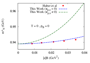
Figure 2: Variation of $m_{N}^{*}$ with $\left|e\right|B$ at zero temperature and zero density. Results with and without the anomalous magnetic moment of nucleons are compared with results from Ref.Haber:2014ula .

We begin this section by obtaining the effective nucleon mass with external magnetic field at zero temperature and zero density. In this case the contribution from $\Sigma_{s}^{\text{(medium)}}=0$. Thus we need to solve the transcendental equation,

$$m_{N}^{*}=m_{N}+\Sigma_{s}^{\text{(vacuum)}}\left(m_{N}^{*}\right)$$ (71)

where, $\Sigma_{s}^{\text{(vacuum)}}\left(m_{N}^{*}\right)$ is given in Eq. (68). At first we neglect the effect of anomalous magnetic moment of nucleons so that the above equation simplifies to

$$m_{N}^{*}=m_{N}+\frac{g^{2}_{\sigma NN}\left(eB\right)^{2}}{12\pi^{2}m_{\sigma}^{2}m_{N}^{*}}$$ (72)

which can be solved analytically to obtain

$$m_{N}^{*}=\frac{1}{2}\left[m_{N}+\sqrt{m_{N}^{2}+\frac{g^{2}_{\sigma NN}\left(eB\right)^{2}}{3\pi^{2}m_{\sigma}^{2}}}\right]~{}.$$ (73)

As can be seen from the above equation, the effective nucleon mass increases monotonically with the increase of $eB$. This enhancement is shown in Fig. 2 where it is also compared with the result from Ref Haber:2014ula . Though the current approach to obtain the effective nucleon mass differs from Ref Haber:2014ula , there exists a noticeable quantitative agreement between the two results in the weak magnetic field regime. Now we include the anomalous magnetic moments of nucleons and solve Eq. (71) numerically. It is found that the incorporation of nucleon magnetic moment further increases the effective mass and this effect remains significant even in case of weak magnetic fields as shown in Fig. 2. In other words, the nucleon magnetic moment favors the magnetic catalysis effect at zero temperature and zero baryon density.

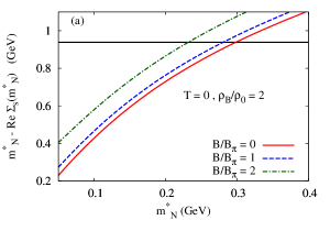
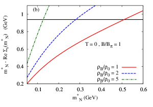
Figure 3: Variation of $m_{N}^{*}-\text{Re}\Sigma_{s}\left(m_{N}^{*}\right)$ with $m_{N}^{*}$ at zero temperature for (a) three different values of magnetic field ($B=0,B_{\pi},2B_{\pi}$) at baryon density $\rho_{\text{B}}=2\rho_{0}$ (b) three different values of baryon density ($\rho_{B}=\rho_{0},2\rho_{0},5\rho_{0}$) at magnetic field ($B=B_{\pi}$). Here $|e|B_{\pi}=m_{\pi}^{2}=0.0196~{}\text{GeV}^{2}$ and $\rho_{0}=0.16~{}\text{fm}^{-3}$. The horizontal black solid line corresponds to $m_{N}^{*}=m_{N}=939$ MeV.

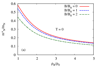
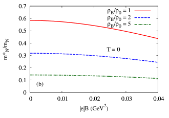
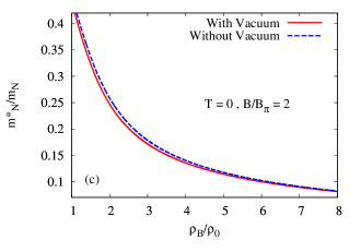
Figure 4: Variation of effective mass of nucleon at zero temperature (a) with baryon density for three different values of magnetic field ($B=0,B_{\pi},2B_{\pi}$). The horizontal axis starts at $\rho_{B}=0.1\rho_{0}$. (b) with magnetic field for three different values of baryon density ($\rho_{B}=\rho_{0},2\rho_{0},5\rho_{0}$). Here $|e|B_{\pi}=m_{\pi}^{2}=0.0196~{}\text{GeV}^{2}$ and $\rho_{0}=0.16~{}\text{fm}^{-3}$. (c) At $B=2B_{\pi}$, the variation of the effective nucleon mass with baryon density is compared with the case where the vacuum contribution is ignored.

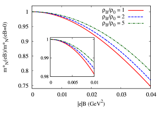
Figure 5: At T=0, the ratio of effective mass $m^{\ast}$ at non-zero $eB$ and at zero $eB$ is plotted as a function of $eB$ for three different values of baryon density ($\rho_{B}=\rho_{0},2\rho_{0},5\rho_{0}$). The inset plot shows the low $eB$ region upto $eB=0.01$ GeV² relevant for neutron star/magnetar case. Here $\rho_{0}=0.16~{}\text{fm}^{-3}$.

Let us now proceed to the study of nucleon effective mass in presence of external magnetic field at at finite baryon density and zero temperature. As can be seen from Eqs. (68)-(69), the scalar self energy $\Sigma_{s}$ is functions of magnetic field $B$ and baryon chemical potential $\mu_{\text{B}}$ of the medium. It is customary to use total baryon density $\rho_{\text{B}}$ instead of $\mu_{\text{B}}$ where

$$\rho_{\text{B}}=4\int\frac{d^{3}p}{\left(2\pi\right)^{3}}\Theta\left(\mu_{\text{B}}-\sqrt{\left|\vec{p}\right|^{2}+m_{N}^{*2}}\right)=\left(\frac{2}{3\pi^{2}}\right)\left[\mu_{\text{B}}^{2}-m_{N}^{*2}\frac{}{}\right]^{3/2}~{}.$$ (74)

Inverting the above equation, we get the baryon chemical potential in terms of the baryon density as

$$\mu_{\text{B}}=\sqrt{\left(\frac{3\pi^{2}}{2}\rho_{\text{B}}\right)^{2/3}+m_{N}^{*2}}~{}.$$ (75)

We have expressed the strength of the magnetic field $B$ with respect to the pion mass scale ($B_{\pi}$) defined as

$$\left|e\right|B_{\pi}=m_{\pi}^{2}=0.0196\text{ GeV}^{2}.$$ (76)

Similarly the total baryon density $\rho_{B}$ is expressed with respect to the normal nuclear matter density $\rho_{0}=0.16$ fm^-3.

Since we will be solving the transcendental Eq. (61), we first plot $m_{N}^{*}-\text{Re}\Sigma_{s}\left(m_{N}^{*}\right)$ as a function of $m_{N}^{*}$ in Fig. 3. Fig. 3-(a) depicts the variation of this quantity at three different values of magnetic field ($B/B_{\pi}=$ 0, 1 and 2) with baryon density $\rho_{B}=2\rho_{0}$ whereas Fig. 3-(b) shows its variation at three different values of total baryon density ($\rho_{B}/\rho_{0}=$ 1, 2 and 3) with magnetic field $B=B_{\pi}$. The intersections of this graphs with the horizontal line corresponding to $m_{N}^{*}=m_{N}=939$ MeV represent the solutions of Eq. (61). We notice from these figures that $\text{Re}\Sigma\left(m_{N}^{*}\right)$ is always less than zero and it monotonically decreases as we increase $m_{N}^{*}$. Also for a particular value of $m_{N}^{*}$, $\text{Re}\Sigma\left(m_{N}^{*}\right)$ decreases with the increase of $B$ and $\rho_{B}$. In Fig. 4-(a), the variation of the effective nucleon mass with baryon density has been shown at three different values of magnetic field ($B=0,B_{\pi},2B_{\pi}$). As can be seen from the figure, $m_{N}^{*}/m_{N}$ decreases with the increase of $\rho_{\text{B}}$ and becomes less than $0.5$ at $\rho_{\text{B}}=2\rho_{0}$. It can be checked that the contribution from the first term within the square brackets in Eq. (69) plays the dominant role in determining the $\rho_{\text{B}}$ as well as the $eB$ dependences of the effective mass whereas the net contribution from all the other terms in $\Sigma_{s}^{\text{(medium)}}$ and $\Sigma_{s}^{\text{(vacuum)}}$ (see Eq. (68)) remains sub-leading throughout. Also, it is clear from Fig. 4-(a) that, with the increase of $|e|B$, the effective mass decreases and the effect of the external magnetic field is more at a lower $\rho_{\text{B}}$ region. At very high $\rho_{\text{B}}(\gtrsim 5\rho_{0})$ it is expected that the effect of $\left|e\right|B$ on nucleon effective mass becomes negligible. However, the conclusions based on the weak field approximation will not be reliable for arbitrary large or small densities as will be discussed later.

In Fig. 4-(b), the variation of $m_{N}^{*}/m_{N}$ with $\left|e\right|B$ is shown at three different values of baryon density ($\rho_{B}=\rho_{0},2\rho_{0},5\rho_{0}$). We find a small decrease in effective nucleon mass with $|e|B$. In order to observe the effect of the vacuum self energy correction to the effective mass of nucleon, we have compared the density variations of $m_{N}^{*}$ with and without the vacuum contribution as shown in Fig. 4(c). Here the external magnetic field is kept fixed at $B=2B_{\pi}$. It has been noticed that the effect of vacuum correction is subleading with respect to the medium contribution at non-zero baryon density and the correction to $m_{N}^{*}$ due to vacuum self energy remains less than 6%. It is also interesting to observe the relative importance of the external magnetic field on the effective nucleon mass as shown in Fig. 5 where the ratio $m_{N}^{*}(eB)/m_{N}^{*}(eB=0)$ is plotted as a function of $eB$ at three different baryon densities( $\rho_{B}=\rho_{0},2\rho_{0},5\rho_{0}$). It can be noticed that $m_{N}^{*}$ decreases by about 25% at a magnetic field $eB\sim 0.04$ GeV². The inset plot shows the lower $eB$ region upto $eB=0.01$ GeV² which corresponds to the typical values of magnetic field expected inside a neutron star/magnetar. At the maximum value $eB=0.01$ GeV², the effective mass of nucleon is found to be lowered by less than 2%.

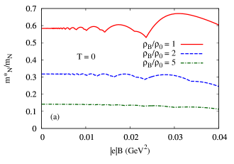
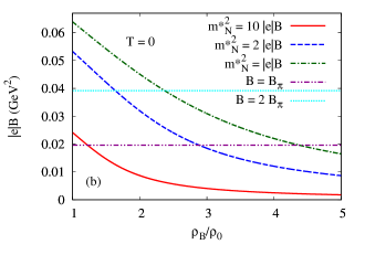
Figure 6: Variation of effective mass of nucleon at zero temperature (a) with baryon density for three different values of magnetic field ($B=0,B_{\pi},2B_{\pi}$). The horizontal axis starts at $\rho_{B}=0.1\rho_{0}$. (b) with magnetic field for three different values of baryon density ($\rho_{B}=\rho_{0},2\rho_{0},5\rho_{0}$). Here $|e|B_{\pi}=m_{\pi}^{2}=0.0196~{}\text{GeV}^{2}$ and $\rho_{0}=0.16~{}\text{fm}^{-3}$.

Until now we have considered that under weak field approximation, the modifications from the non-vanishing anomalous magnetic moment arise only through the effective mass. Moreover, it is assumed that the modification in the expression of proton density as a summation over Landau levels can also be ignored for weak external fields. The motivation behind this approximation lies in the fact that with smaller values of external field, the Landau levels become more and more closely spaced giving rise to a continuum at $eB\rightarrow 0$. In that case, the summations that appeared due to the Landau quantization, can be replaced by the corresponding momentum integrals giving rise to exactly similar expression for proton and neutron density in isospin symmetric matter. As a result, the expression of baryon density as given in Eq. (74) remains to be valid even in presence of $eB$ as long as the external fields are sufficiently weak to make the summation to integral conversion plausible. It is advantageous to use this approximate expression to obtain the effective mass of the nucleons as, in this case, $\mu_{\text{B}}$ can be analytically expressed in terms of $\rho_{\text{B}}$ providing useful simplifications in the numerics. However, to check the validity of the approximations, it is reasonable to incorporate this magnetic modifications in the expression for the net baryon density which now becomes Aguirre1 ; Aguirre2

$$\rho_{\text{B}} = \sum_{s\in\{\pm 1\}}\int\frac{d^{3}p}{\left(2\pi\right)^{3}}\Theta\left\{\mu_{\text{B}}-\sqrt{p_{z}^{2}+\left(\sqrt{m_{N}^{*2}-p_{\perp}^{2}}-s\kappa_{\text{n}}B\right)^{2}}\right\}$$ (77)

$$\hskip 28.45274pt+\frac{eB}{(2\pi)^{2}}\sum_{s\in\{\pm 1\}}\sum_{n=0}^{\infty}(1-\delta_{0}^{n}\delta_{-1}^{s})\int_{-\infty}^{\infty}dp_{z}\Theta\left\{\mu_{\text{B}}-\sqrt{p_{z}^{2}+\left(\sqrt{m_{N}^{*2}+2n|e|B}-s\kappa_{\text{p}}B\right)^{2}}\right\}.$$

Performing the momentum integral in the above equation, we obtain

$$\rho_{\text{B}} = \sum_{s\in\{\pm 1\}}\frac{1}{12\pi^{2}}\left[3\pi\mu_{\text{B}}^{2}s\kappa_{\text{n}}B+2\sqrt{\mu_{\text{B}}^{2}-(m_{N}^{*}-s\kappa_{\text{n}}B)^{2}}\left\{\frac{}{}2\mu_{\text{B}}^{2}-2m_{N}^{*2}+m_{N}^{*}s\kappa_{\text{n}}B+(s\kappa_{\text{n}}B)^{2}\right\}\right.$$ (78)

$$\left.+6\mu_{\text{B}}^{2}s\kappa_{\text{n}}B\tan^{-1}\left\{\frac{s\kappa_{\text{n}}B-m_{N}^{*}}{\sqrt{\mu_{\text{B}}^{2}-(m_{N}^{*}-s\kappa_{\text{n}}B)^{2}}}\right\}\right]$$

$$+\frac{eB}{2\pi^{2}}\sum_{s\in\{\pm 1\}}\sum_{n=0}^{n_{\text{max}}}(1-\delta_{0}^{n}\delta_{-1}^{s})\sqrt{\mu_{\text{B}}^{2}-\left(\sqrt{m_{N}^{*2}+2n|e|B}-s\kappa_{\text{p}}B\right)^{2}}$$

where, $n_{\text{max}}=\left[\frac{(\mu_{\text{B}}+s\kappa_{\text{p}}B)^{2}-m_{N}^{*2}}{2|e|B}\right]$ in which $\left[x\right]=$ greatest integer less than or equal to $x$. The above equation can not be inverted analytically in order to express $\mu_{B}$ as a function of $\rho_{B}$ which was possible for $eB=0$ case (see Eq. (75)). Thus we invert the equation numerically to obtain $\mu_{B}=\mu_{B}(\rho_{B},eB)$. Using the above modified $\rho_{B}$, we have re-plotted the effective mass variation with the external field for the same set of densities $\rho_{B}=\rho_{0},2\rho_{0}$ and $5\rho_{0}$ as shown in Fig. 6. The oscillating behaviour is consistent with Ref. Haber:2014ula . Comparison with Fig.4(b) suggests that the usual baryon density expression provides the average qualitative behaviour reasonably well even in presence of external magnetic field as long as the background field strength is small and the agreement is more pronounced in higher density regime. However, going to arbitrary large densities is restricted by the assumption of weak field expansion of the propagator which demands the external $eB$ to be much smaller than $m_{N}^{\ast 2}$. Now, apart from the external magnetic field, this effective mass depends on density as well and more importantly, the dependence is of decreasing nature. Thus, even if one starts with a constant $eB$ much lower than $m_{N}^{\ast 2}$, the decreasing trend of $m_{N}^{\ast}$ with density invalidates this basic weak field assumption at some higher $\rho_{\text{B}}$ value for which $m_{N}^{\ast 2}$ becomes comparable with the constant $eB$ used. To estimate this density value, we fix the maximum possible value of $eB$ to be considered as a fraction times $m_{N}^{\ast 2}$ where the fraction is chosen to be 0.5 and 0.1. The corresponding variation with respect to $\rho_{\text{B}}$ are shown in Fig.6(b) where the case $eB=m_{N}^{\ast 2}$ is also plotted for comparison. Each of these curves in fact serves the purpose of a boundary and for a given value of $\rho_{\text{B}}$, only those $eB$ values are allowed which lie below it. The horizontal lines denote the constant magnetic field values used in this work. It is clear from the figure that, once we have chosen the maximum $eB$ curve( say $eB=0.5m_{N}^{\ast 2}$ curve), its intersection with each horizontal lines provides the maximum density ( i.e around $3\rho_{0}$ for $B=B_{\pi}$ and around $1.8\rho_{0}$ for $B=2B_{\pi}$) up to which the $eB$ value corresponding to that line can be considered as ‘weak’.

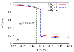
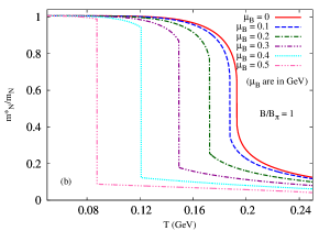
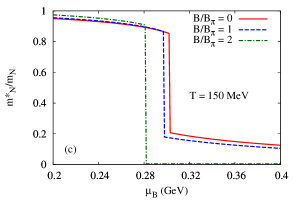
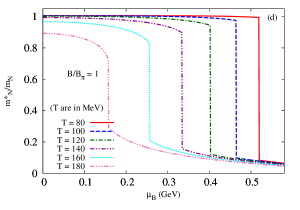
Figure 7: Variation of effective mass of nucleon with temperature (a) at $\mu_{\text{B}}$=300 MeV for three different values $B$ ($0,B_{\pi}$ and $2B_{\pi}$) (b) at $B=B_{\pi}$ for six different values $\mu_{\text{B}}$ (0, 100, 200, 300, 400 and 500 MeV). Variation of effective mass of nucleon with baryon chemical potential (a) at $T$=150 MeV for three different values of magnetic field ($B=0,B_{\pi},2B_{\pi}$) (b) at $B=B_{\pi}$ for six different value of $T$ = 80, 100, 120, 140, 160 and 180 MeV. Here $|e|B_{\pi}=m_{\pi}^{2}=0.0196~{}\text{GeV}^{2}$.

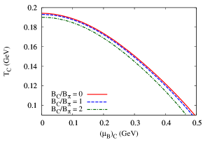
Figure 8: Phase diagram for vacuum to nuclear medium phase transition in Walecka model for three different values of $B$ ($0,B_{\pi}$ and $2B_{\pi}$).

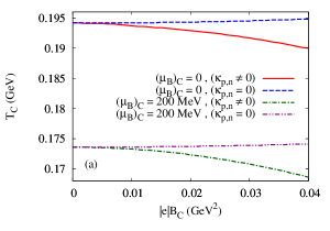
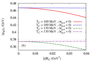
Figure 9: (a) Variation of transition temperature with magnetic field at two different values of $\mu_{\text{B}}$ (0 and 200 MeV). (b) Variation of transition baryon chemical potential with magnetic field at two different values of $T$ (100 and 130 MeV). Cases with and without the ANM of nucleons are shown separately.

We now turn on the temperature and study the variation of $m_{N}^{*}/m_{N}$ with temperature and baryon chemical potential in Fig. 7. Fig. 7-(a) depicts the variation of $m_{N}^{*}/m_{N}$ with $T$ at at $\mu_{\text{B}}$=300 MeV and at three different values $B$ ($0,B_{\pi}$ and $2B_{\pi}$) whereas Fig. 7-(b) shows its variation at $B=B_{\pi}$ and at six different values $\mu_{\text{B}}$ (0, 100, 200, 300, 400 and 500 MeV). As can be seen from the figure, that the effective nucleon mass suffers a sudden decrease at a particular temperature corresponding to the vacuum to nuclear medium phase transition Negele:1986bp ; Haber:2014ula . We call this transition temperature as $T_{C}$ which we calculate numerically from the slope of of these plots. As can be seen from Fig. 7-(a), $T_{C}$ decreases with the increase of $B$, which may be identified as IMC in Walecka model. In Fig. 7-(b), we observe that $T_{C}$ decreases with the increase of $\mu_{\text{B}}$. The corresponding variation of $m_{N}^{*}/m_{N}$ with $\mu_{\text{B}}$ is shown in Fig. 7-(b) and (c). Analogous to the upper panels, we see the phase transition at a particular $\mu_{\text{B}}$ and we call this transition chemical potential as $\left(\mu_{\text{B}}\right)_{C}$. As can be seen in the graphs, $\left(\mu_{\text{B}}\right)_{C}$ decreases with the increase in $B$ and $T$.

The behaviour of $T_{C}$ and $\left(\mu_{\text{B}}\right)_{C}$ at different $B$ can be seen in Fig. 8, where, we have presented the phase diagram for the vacuum to nuclear medium phase transition at three different values of $B$ ($0,B_{\pi}$ and $2B_{\pi}$). With the increase in $\left(\mu_{\text{B}}\right)_{C}$, $T_{C}$ decreases and vice-versa. Also, with the increase in $B$, the phase boundary in this $T-\mu_{\text{B}}$ plane moves towards lower values of $T$ and $\mu_{\text{B}}$ showing IMC.

We conclude this section by presenting the variation of $T_{C}$ and $\left(\mu_{\text{B}}\right)_{C}$ with external magnetic field in Fig. 9. Fig. 9-(a) shows the variation of $T_{C}$ with $|e|B$ at two different values of $\mu_{\text{B}}$ (0 and 200 MeV) whereas Fig. 9-(b) shows the corresponding variation at at two different values of $T$ (100 and 130 MeV). As already discussed, both the $T_{C}$ and $\left(\mu_{\text{B}}\right)_{C}$ decreases with the increase in $B$ characterizing the IMC effect. However, once the anomalous magnetic moment is ignored, $T_{C}$ as well as $\left(\mu_{\text{B}}\right)_{C}$ can be observed to slowly increase with the external magnetic field showing MC as expected Haber:2014ula .

VI Summary

In this article we have used the Walecka model to study the vacuum to nuclear matter phase transition in presence of a weak and constant background magnetic field within mean field approximation. In case of weak magnetic field, the nucleon propagators are derived as a series in powers of $qB$ and $\kappa B$ where $q$ and $\kappa$ represents the charge and the anomalous magnetic moment of the nucleons. The effective mass of the nucleon ($m_{N}^{*}$) is obtained from the pole of the nucleon propagator self-consistently. At zero temperature and zero density, the incorporation of anomalous magnetic moment is shown to favour the effective mass enhancement with the external magnetic field. The functional dependence of $m_{N}^{*}$ on the background field is extended to the case of non-zero nuclear density and further extended to the finite temperature regime. It is observed that in the case of vanishing temperature within dense nuclear medium, the effective mass decreases with the background magnetic field and this trend is shown to survive in case of non-zero temperature as well. Moreover, there exists a particular temperature (denoted by $T_{C}$ in the text) for which the effective nucleon mass suffers a sudden decrease corresponding to the vacuum to nuclear medium phase transition. It has been shown that this critical temperature decreases with the increase of $B$ which can be identified as inverse magnetic catalysis in Walecka model whereas the opposite behaviour is obtained in case of vanishing magnetic moment. Thus, it can be inferred that in presence of external magnetic field, the anomalous magnetic moment of the nucleons plays a crucial role in characterizing the nature of vacuum to nuclear matter transition at finite temperature and density.It should be mentioned here that Haber et.al Haber:2014ula had speculated that the incorporation of anomalous magnetic moment could counteract the effect of magnetic catalysis haber37 . Our study not only supports the speculation but also concludes that the effect is significant enough to alter the qualitative behaviour of the nucleon effective mass even in weak magnetic field regime. However, it should be noted here that the weak field approximation actually restricts the regime of validity of the present study as discussed in detail in the text. The maximum value of the external magnetic field used in the present study is taken to be 0.04 GeV² and it has been argued to be considered as ‘weak’ only up to density 1.8 $\rho_{0}$ where the assumption of ‘weakness’ is fixed by the condition that the chosen external field has to remain less than 50% of the effective mass. One should also notice that in case of Walecka model, MC or IMC can only be seen indirectly. Similar studies in extended linear sigma model might be interesting as in that case the possibility of (approximate) chiral symmetry restoration is incorporated within the model framework. However, we should also mention that in case of zero magnetic moment, only the quantitative difference in the behaviour of the effective mass is found to be attributed to the presence of the chiral partners Haber:2014ula whereas the qualitative behaviour which has been the main interest throughout the article seems to show model independence. Before applying the present result to obtain the characteristics of compact stars such as mass radius relationship or the equation of state, beta equilibrium and charge neutrality conditions have to be properly incorporated which lies beyond the scope of the present study.

Appendix A Calculation of $\Sigma_{s}^{\text{(vacuum)}}$

We have from Eq. (65),

$$\Sigma_{s}^{\text{(vacuum)}}=\left(\frac{g^{2}_{\sigma NN}}{m_{\sigma}^{2}}\right)\text{Re}~{}i\int\frac{d^{d}p}{\left(2\pi\right)^{d}}\hat{T}\left(p,m_{N}^{*},m_{1}\right)\left.\frac{1}{p^{2}-m_{1}^{2}+i\epsilon}\right|_{m_{1}=m_{N}^{*},d\rightarrow 4}$$ (79)

In order to perform the $d^{4}p$ integration, we use the following identities Peskin:1995ev

$$\int\frac{d^{d}p}{\left(2\pi\right)^{d}}\left(\frac{1}{p^{2}-\Delta}\right) = \frac{-i}{\left(4\pi\right)^{d/2}}\Gamma\left(1-\frac{d}{2}\right)\left(\frac{1}{\Delta}\right)^{1-d/2}$$ (80)

$$\int\frac{d^{d}p}{\left(2\pi\right)^{d}}\left(\frac{p_{\perp}^{2}}{p^{2}-\Delta}\right) = \frac{i}{\left(4\pi\right)^{d/2}}\left(\frac{d}{4}\right)\Gamma\left(-\frac{d}{2}\right)\left(\frac{1}{\Delta}\right)^{-d/2}$$ (81)

$$\int\frac{d^{d}p}{\left(2\pi\right)^{d}}\left(\frac{p_{\parallel}^{2}}{p^{2}-\Delta}\right) = \frac{i}{\left(4\pi\right)^{d/2}}\left(\frac{d}{4}\right)\Gamma\left(-\frac{d}{2}\right)\left(\frac{1}{\Delta}\right)^{-d/2}$$ (82)

$$\int\frac{d^{d}p}{\left(2\pi\right)^{d}}\left(\frac{p^{2}}{p^{2}-\Delta}\right) = \frac{i}{\left(4\pi\right)^{d/2}}\left(\frac{d}{2}\right)\Gamma\left(-\frac{d}{2}\right)\left(\frac{1}{\Delta}\right)^{-d/2}$$ (83)

so that, Eq. (79) will become

$$\Sigma_{s}^{\text{(vacuum)}} = \text{Re}\Sigma_{s}^{\text{(pure vacuum)}}+\Sigma_{s}^{\text{(divergent)}}+\Sigma_{s}^{\text{(regular)}}$$ (84)

where $\text{Re}\Sigma_{s}^{\text{(pure vacuum)}}$ is the ultra-violate divergent pure vacuum contribution given in Eq. 60 and

$$\Sigma_{s}^{\text{(divergent)}} = -\left(\frac{g^{2}_{\sigma NN}}{4\pi^{2}m_{\sigma}^{2}}\right)\left\{\left(\kappa_{\text{p}}B\right)^{2}m_{N}^{*}+\left(\kappa_{\text{n}}B\right)^{2}m_{N}^{*}\frac{}{}+\frac{}{}\left(\left|e\right|B\right)\left(\kappa_{\text{p}}B\right)\right\}\left.\Gamma\left(2-\frac{d}{2}\right)\left(\frac{1}{m_{N}^{*2}}\right)^{2-d/2}\right|_{d\rightarrow 4}$$ (85)

$$\Sigma_{s}^{\text{(regular)}} = \left(\frac{g^{2}_{\sigma NN}}{4\pi^{2}m_{\sigma}^{2}}\right)\left[\frac{\left(eB\right)^{2}}{3m_{N}^{*}}+\frac{1}{2}\left\{\left(\kappa_{\text{p}}B\right)^{2}m_{N}^{*}+\left(\kappa_{\text{n}}B\right)^{2}m_{N}^{*}\frac{}{}+\frac{}{}\left(\left|e\right|B\right)\left(\kappa_{\text{p}}B\right)\right\}\right]~{}.$$ (86)

In this case also, we will neglect the pure vacuum contribution $\text{Re}\Sigma_{s}^{(\text{pure vacuum})}$ which is equivalent to use the MFT. We now extract the divergence of $\Sigma_{s}^{\text{(divergent)}}$ from the pole of the Gamma function and use $\overline{\text{MS}}$ scheme to obtain,

$$\Sigma_{s}^{\text{(divergent)}} = \left(\frac{g^{2}_{\sigma NN}}{4\pi^{2}m_{\sigma}^{2}}\right)\left\{\left(\kappa_{\text{p}}B\right)^{2}m_{N}^{*}+\left(\kappa_{\text{n}}B\right)^{2}m_{N}^{*}\frac{}{}+\frac{}{}\left(\left|e\right|B\right)\left(\kappa_{\text{p}}B\right)\right\}\ln\left(\frac{m_{N}^{*2}}{\Lambda}\right)$$ (87)

where $\Lambda$ is a scale of dimension GeV². Its value is fixed from the condition $\Sigma_{s}^{\text{(divergent)}}\left(m_{N}^{*}=m_{N}\right)=0$, which gives $\Lambda=m_{N}^{2}$. So the final expression of $\Sigma_{s}^{\text{(vacuum)}}$ becomes

$$\Sigma_{s}^{\text{(vacuum)}} = \left(\frac{g^{2}_{\sigma NN}}{4\pi^{2}m_{\sigma}^{2}}\right)\left[\frac{\left(eB\right)^{2}}{3m_{N}^{*}}+\left\{\left(\kappa_{\text{p}}B\right)^{2}m_{N}^{*}+\left(\kappa_{\text{n}}B\right)^{2}m_{N}^{*}+\left(\left|e\right|B\right)\left(\kappa_{\text{p}}B\right)\right\}\left\{\frac{1}{2}+2\ln\left(\frac{m_{N}^{*}}{m_{N}}\right)\right\}\right]~{}$$ (88)

Appendix B Calculation of $\Sigma_{s}^{\text{(medium)}}$

We have from Eq. (66)

$$\Sigma_{s}^{\text{(medium)}} = -\left(\frac{g^{2}_{\sigma NN}}{m_{\sigma}^{2}}\right)\int\frac{d^{4}p}{\left(2\pi\right)^{4}}\hat{T}\left(p,m_{N}^{*},m_{1}\right)\left.\frac{}{}2\pi\eta\left(p\cdot u\right)\delta\left(p^{2}-m_{1}^{2}\right)\right|_{m_{1}=m_{N}^{*}}$$ (89)

where $\hat{T}\left(p,m_{N}^{*},m_{1}\right)$ is given in Eq. (67). Using Eqs. (35) and (36), we can write the above equation as,

$$\Sigma_{s}^{\text{(medium)}} = -\left(\frac{g^{2}_{\sigma NN}}{m_{\sigma}^{2}}\right)\int\frac{d^{3}p}{\left(2\pi\right)^{3}}\int_{-\infty}^{+\infty}dp^{0}\hat{T}\left(p^{0},\vec{p},m_{N}^{*},m_{1}\right)\left(\frac{1}{2\omega_{1}}\right)\times$$

$$\left[\frac{}{}f_{+}\left(\omega_{1}\right)\delta\left(p^{0}-\omega_{1}\right)+f_{-}\left(\omega_{1}\right)\delta\left(p^{0}+\omega_{1}\right)\right]_{m_{1}=m_{N}^{*}}$$

where $\omega_{1}=\sqrt{\vec{p}^{2}+m_{1}^{2}}$. Performing the $dp^{0}$ integration using the Dirac delta functions and noting that $\hat{T}\left(p^{0},\vec{p},m_{N}^{*},m_{1}\right)$ is an even function of $p^{0}$, we get

$$\Sigma_{s}^{\text{(medium)}} = -\left(\frac{g^{2}_{\sigma NN}}{2m_{\sigma}^{2}}\right)\int\frac{d^{3}p}{\left(2\pi\right)^{3}}\hat{T}\left(p^{0}=\Omega_{p},\vec{p},m_{N}^{*},m_{1}\right)\left(\frac{1}{\omega_{1}}\right)\times\left[\frac{}{}f_{+}\left(\omega_{1}\right)+f_{-}\left(\omega_{1}\right)\right]_{m_{1}=m_{N}^{*}}$$ (90)

Substituting Eq. (67) into (90) and performing the angular integration we get,

$$\Sigma_{s}^{\text{(medium)}} = -\left(\frac{g^{2}_{\sigma NN}}{8\pi^{2}m_{\sigma}^{2}}\right)\int_{0}^{\infty}\left|\vec{p}\right|^{2}d\left|\vec{p}\right|\hat{B}\left(\vec{p},m_{N}^{*},m_{1}\right)\left(\frac{1}{\omega_{1}}\right)\times\left[\frac{}{}f_{+}\left(\omega_{1}\right)+f_{-}\left(\omega_{1}\right)\right]_{m_{1}=m_{N}^{*}}$$ (91)

where,

$$\hat{B}\left(\vec{p},m_{N}^{*},m_{1}\right)=16m_{N}^{*}+\frac{32}{3}\left(eB\right)^{2}m_{N}^{*}\left|\vec{p}\right|^{2}\hat{A}_{3}+16\left(2m_{N}^{*2}+\frac{4}{3}\left|\vec{p}\right|^{2}\right)\times$$

$$\left\{m_{N}^{*}\left(\kappa_{\text{p}}B\right)^{2}+m_{N}^{*}\left(\kappa_{\text{n}}B\right)^{2}+\left(\left|e\right|B\right)\left(\kappa_{\text{p}}B\right)\right\}\hat{A}_{2}~{}.$$ (92)

B.1 Zero Temperature Case

From Eq. (36) we have at $T=0$,

$$\lim\limits_{T\rightarrow 0}f_{\pm}\left(\omega_{1}\right)=\Theta\left(\pm\mu_{\text{B}}-\omega_{1}\right)$$ (93)

where $\mu_{\text{B}}$ is the baryon chemical potential of the medium. Substituting Eq. (93) into (91) we get,

$$\Sigma_{s}^{\text{(medium)}} = -\left(\frac{g^{2}_{\sigma NN}}{8\pi^{2}m_{\sigma}^{2}}\right)\int_{0}^{\infty}\left|\vec{p}\right|^{2}d\left|\vec{p}\right|\left.\hat{B}\left(\vec{p},m_{N}^{*},m_{1}\right)\frac{1}{\omega_{1}}\Theta\left(\mu_{\text{B}}-\omega_{1}\right)\right|_{m_{1}=m_{N}^{*}}~{}.$$ (94)

The the $d\left|\vec{p}\right|$ integration of the above equation can be evaluated analytically using the following identities

$$I_{2}\left(\mu,m\right) = \int_{0}^{\sqrt{\mu^{2}-m^{2}}}\frac{\left|\vec{p}\right|^{2}d\left|\vec{p}\right|}{\sqrt{\left|\vec{p}\right|^{2}+m^{2}}}=\frac{1}{2}\left[\mu\sqrt{\mu^{2}-m^{2}}+m^{2}\ln\left\{\frac{m}{\mu+\sqrt{\mu^{2}-m^{2}}}\right\}\right]$$ (95)

$$I_{4}\left(\mu,m\right) = \int_{0}^{\sqrt{\mu^{2}-m^{2}}}\frac{\left|\vec{p}\right|^{4}d\left|\vec{p}\right|}{\sqrt{\left|\vec{p}\right|^{2}+m^{2}}}=\frac{1}{8}\left[\mu\left(2\mu^{2}-5m^{2}\right)\sqrt{\mu^{2}-m^{2}}-3m^{4}\ln\left\{\frac{m}{\mu+\sqrt{\mu^{2}-m^{2}}}\right\}\right]$$ (96)

and we get,

$$\Sigma_{s}^{\text{(medium)}} = -\left(\frac{2g^{2}_{\sigma NN}}{\pi^{2}m_{\sigma}^{2}}\right)\left[m_{N}^{*}I_{2}\left(\mu_{\text{B}},m_{1}\right)+\frac{2}{3}\left(eB\right)^{2}m_{N}^{*}\hat{A}_{3}I_{4}\left(\mu_{\text{B}},m_{1}\right)\right.$$ (97)

$$\left.+2\left\{m_{N}^{*}\left(\kappa_{\text{p}}B\right)^{2}+m_{N}^{*}\left(\kappa_{\text{n}}B\right)^{2}+\left(\left|e\right|B\right)\left(\kappa_{\text{p}}B\right)\right\}\left\{m_{N}^{*2}\hat{A}_{2}I_{2}\left(\mu_{\text{B}},m_{1}\right)+\frac{1}{3}\hat{A}_{2}I_{4}\left(\mu_{\text{B}},m_{1}\right)\right\}\right]_{m_{1}=m_{N}^{*}}~{}.$$

It is now trivial to check that

$$\left.\frac{}{}\hat{A}_{2}I_{2}\left(\mu,m_{1}\right)\right|_{m_{1}=m_{N}^{*}} = \left.\frac{}{}2\hat{A}_{3}I_{4}\left(\mu,m_{1}\right)\right|_{m_{1}=m_{N}^{*}}=\frac{\mu}{8m_{N}^{*2}\sqrt{\mu^{2}-m_{N}^{*2}}}=C_{1}\left(\mu,m_{N}^{*}\right)~{}~{}~{}\text{(say)}$$ (98)

$$\left.\frac{}{}\hat{A}_{2}I_{4}\left(\mu,m_{1}\right)\right|_{m_{1}=m_{N}^{*}} = -\left(\frac{3}{8}\right)\ln\left\{\frac{m_{N}^{*}}{\mu+\sqrt{\mu^{2}-m_{N}^{*2}}}\right\}=C_{2}\left(\mu,m_{N}^{*}\right)~{}~{}~{}\text{(say)}~{}.$$ (99)

So finally $\Sigma_{s}^{\text{(medium)}}$ becomes,

$$\Sigma_{s}^{\text{(medium)}} = -\left(\frac{2g^{2}_{\sigma NN}}{\pi^{2}m_{\sigma}^{2}}\right)\left[m_{N}^{*}I_{2}\left(\mu_{\text{B}},m_{N}^{*}\right)+\frac{1}{3}\left(eB\right)^{2}m_{N}^{*}C_{1}\left(\mu_{\text{B}},m_{N}^{*}\right)\right.$$ (100)

$$\left.+2\left\{m_{N}^{*}\left(\kappa_{\text{p}}B\right)^{2}+m_{N}^{*}\left(\kappa_{\text{n}}B\right)^{2}+\left(\left|e\right|B\right)\left(\kappa_{\text{p}}B\right)\right\}\left\{m_{N}^{*2}C_{1}\left(\mu_{\text{B}},m_{N}^{*}\right)+\frac{1}{3}C_{2}\left(\mu_{\text{B}},m_{N}^{*}\right)\right\}\right]~{}.$$

B.2 Finite Temperature Case

At finite temperature, the $d\left|\vec{p}\right|$ integration in Eq. (91) can not be performed analytically. We simplify the expression by evaluating the derivatives with respect to $m_{1}^{2}$ explicitly. For this we use the following results

$$\left[\frac{f_{\pm}\left(\omega_{1}\right)}{\omega_{1}}\right]_{m_{1}=m_{N}^{*}} = \frac{N^{p}_{\pm}}{\Omega_{p}}=\tilde{C}_{1}^{\pm p}~{}~{}~{}\text{(say)}$$ (101)

$$\hat{A}_{2}\left[\frac{f_{\pm}\left(\omega_{1}\right)}{\omega_{1}}\right]_{m_{1}=m_{N}^{*}} = \frac{N^{p}_{\pm}}{8\Omega_{p}^{5}}\left[3+3\left(1-N^{p}_{\pm}\right)\beta\Omega_{p}+\left\{1-3N^{p}_{\pm}+2\left(N^{p}_{\pm}\right)^{2}\right\}\beta^{2}\Omega_{p}^{2}\right]=\tilde{C}_{2}^{\pm p}~{}~{}~{}\text{(say)}$$ (102)

$$\hat{A}_{3}\left[\frac{f_{\pm}\left(\omega_{1}\right)}{\omega_{1}}\right]_{m_{1}=m_{N}^{*}} = \frac{N^{p}_{\pm}}{48\Omega_{p}^{7}}\left[15+15\left(1-N^{p}_{\pm}\right)\beta\Omega_{p}+6\left\{1-3N^{p}_{\pm}+2\left(N^{p}_{\pm}\right)^{2}\right\}\beta^{2}\Omega_{p}^{2}\right.$$ (103)

$$\left.+\left\{1-7N^{p}_{\pm}+12\left(N^{p}_{\pm}\right)^{2}-6\left(N^{p}_{\pm}\right)^{3}\right\}\beta^{3}\Omega_{p}^{3}\right]=\tilde{C}_{3}^{\pm p}~{}~{}~{}\text{(say)}$$

and obtain from Eq. (91)

$$\Sigma_{s}^{\text{(medium)}} = -\left(\frac{2g^{2}_{\sigma NN}}{\pi^{2}m_{\sigma}^{2}}\right)\int_{0}^{\infty}\left|\vec{p}\right|^{2}d\left|\vec{p}\right|\left[m_{N}^{*}\left(\tilde{C}_{1}^{+p}+\tilde{C}_{1}^{-p}\right)+\frac{2}{3}m_{N}^{*}\left(eB\right)^{2}\left|\vec{p}\right|^{2}\left(\tilde{C}_{3}^{+p}+\tilde{C}_{3}^{-p}\right)\right.$$ (104)

$$\left.+2\left(m_{N}^{*2}+\frac{2}{3}\left|\vec{p}\right|^{2}\right)\left\{m_{N}^{*}\left(\kappa_{\text{p}}B\right)^{2}+m_{N}^{*}\left(\kappa_{\text{n}}B\right)^{2}+\left(\left|e\right|B\right)\left(\kappa_{\text{p}}B\right)\right\}\left(\tilde{C}_{2}^{+p}+\tilde{C}_{2}^{-p}\right)\right]$$

References

- (1) D. Kharzeev, K. Landsteiner, A. Schmitt and Ho-Ung Yee, Lec.Notes in Phys 871.
- (2) J. M. Lattimer and M. Prakash, Phys. Rep. 442, 109(2007).
- (3) E. J Ferrer, V. de la Incera and C. Manuel, Phys. Rev. Lett. 95, 152002 (2005); Nucl. Phys. B747, 88 (2006).
- (4) E. J Ferrer and V. de la Incera, Phys. Rev. D 76, 045011 (2007).
- (5) K. Fukushima and H. J. Warringa, Phys. Rev. Lett. 100, 032007 (2008).
- (6) J. L. Noronha and I. A. Shovkovy Phys. Rev. D 76, 105030 (2007).
- (7) B. Feng, D.-F. Hou, H.-C. Ren and P.-P. Wu, Phys. Rev. Lett. 105, 042001 (2010)
- (8) S. Fayazbakhsh and N. Sadooghi, Phys. Rev. D 82, 045010 (2010); 83, 025026 (2011).
- (9) V. Skokov, A. Y. Illarionov and V. Toneev, Int. J. Mod. Phys. A 24, 5925(2009)
- (10) T. Vachaspati, Phys. Lett. B 265, 258(1991).
- (11) M. D’Elia, S. Mukherjee and F. Sanfilippo, Phys. Rev. D 82, 051501 (2010).
- (12) M. D’Elia and F. Negro, Phys. Rev. D 83, 114028 (2011).
- (13) J. K. Boomsma and D. Boer, Phys. Rev. D 81, 074005 (2010).
- (14) B. Chatterjee, H. Mishra and A. Mishra, Phys. Rev. D 84, 014016 (2011).
- (15) S. S. Avancini, D. P. Menezes and C. Providencia, Phys. Rev. C 83, 065805 (2011).
- (16) M. Frasca and M. Ruggieri, Phys. Rev. D 83, 094024 (2011).
- (17) A. Rabhi and C. Providencia, Phys. Rev. C 83, 055801 (2011).
- (18) R. Gattto and M. Ruggieri, Phys. Rev. D 82, 054027 (2010); D 83, 034016 (2011).
- (19) K. Kashiwa, Phys. Rev. D 83,, 117901 (2011).
- (20) J. O. Andersen and R. Khan, Phys. Rev. D 85, 065026 (2012).
- (21) J. O. Andersen and A. Tranberg, J. High Energy Phys. 08 002 (2012).
- (22) A. J. Mizhar, M. N. Chernodub and E. S. Fraga, Phys. Rev. D 82, 105016 (2010).
- (23) V. Skokov, Phys. Rev. D 85, 034026 (2012).
- (24) D. C. Duarte, R. L. S. Farias and R. O. Ramos, Phys. Rev. D 84, 083525 (2011).
- (25) E. S. Fraga and L. F. Palhares, Phys. Rev. D 86 016008 (2012).
- (26) G. S. Bali, F. Bruckmann, G. Endrodi, Z. Fodor, S. D. Katz, S. Krieg, A. Schafer, K. K. Szabo, J. High Energy Phys. 02 044 (2012).
- (27) G. S. Bali, F. Bruckmann, G. Endrodi, Z. Fodor, S. D. Katz and A. Schafer, Phys.Rev. D 86, 071502 (2012).
- (28) G. S. Bali, F. Bruckmann, G. Endrodi, F. Gruber, A. Schaefer, J. High Energy Phys. 04 130 (2013).
- (29) V. G. Bornyakov, P. V. Buividovich, N. Cundy, O. A. Kochetkov, and A. Schäfer, Phys. Rev. D 90, 034501 (2014).
- (30) F. Bruckmann, G. Endrodi, T. G. Kovacs, J. High Energy Phys. 04 112 (2013).
- (31) J. O. Andersen and W. R. Naylor, Rev. Mod. Phys. 88, 025001.
- (32) S. Mao, Phys. Lett. B 758, 195 (2016).
- (33) A. Haber, F. Preis and A. Schmitt, Phys. Rev. D 90, no. 12, 125036 (2014) doi:10.1103/PhysRevD.90.125036 [arXiv:1409.0425 [nucl-th]].
- (34) J. D. Walecka, Ann. Phys. (N. Y.) 83, 491 (1974)
- (35) A. Broderick, M. Prakash, and J. M. Lattimer, Astrophys. J. 537, 351 (2000).
- (36) A. E. Broderick, M. Prakash, and J. M. Lattimer, Phys. Lett. B 531, 167 (2002).
- (37) M. Sinha, B. Mukhopadhyay, and A. Sedrakian, Nucl. Phys. A 898, 43 (2013).
- (38) A. Rabhi, P. K. Panda, and C. Providência, Phys. Rev. C 84, 035803 (2011).
- (39) V. Dexheimer, R. Negreiros, and S. Schramm, Eur. Phys. J. A 48, 189 (2012).
- (40) F. Preis, A. Rebhan, and A. Schmitt, J. Phys. G 39, 054006 (2012).
- (41) J. Dong, W. Zuo, and J. Gu, Phys. Rev. D 87, 103010 (2013).
- (42) R. C. R. de Lima, S. S. Avancini, and C. Providência, Phys. Rev. C 88, 035804 (2013).
- (43) R. Casali, L. B. Castro, and D. P. Menezes, Phys. Rev. C 89, 015805 (2014).
- (44) F. Preis, A. Rebhan, and A. Schmitt, J. High Energy Phys. 2011, 033.
- (45) E. J. Ferrer, V. de la Incera, D. M. Paret, A. P. Martinez and A. Sanchez, Phys. Rev. D 91, 085041 (2015).
- (46) A. Ayla, A. Sa ′ nchez, G.Piccinelli, and S.Sahu, Phys. Rev. D 71, 023004 (2005).
- (47) J. F. Nieves, Phys. Rev. D 70, 073001 (2004) doi:10.1103/PhysRevD.70.073001 [hep-ph/0403121].
- (48) J. F. Nieves and P. B. Pal, Phys. Rev. D 73, 105003 (2006) doi:10.1103/PhysRevD.73.105003 [hep-ph/0603024].
- (49) A. Bandyopadhyay and S. Mallik, Phys. Rev. D 95, no. 7, 074019 (2017) doi:10.1103/PhysRevD.95.074019 [arXiv:1704.01364 [hep-ph]].
- (50) S. Mallik and S. Sarkar, “Hadrons at Finite Temperature,” Cambridge University Press.
- (51) J. C. D’Olivo, J. F. Nieves and S. Sahu, Phys. Rev. D 67, 025018 (2003) doi:10.1103/PhysRevD.67.025018 [hep-ph/0208146].
- (52) B. D. Serot and J. D. Walecka, in Advances in Nuclear Physics, edited by J. Negele and E. Vogt (Plenum Press, New York, 1986), Vol. 16, p. 1–327.
- (53) J. Alam, S. Sarkar, P. Roy, T. Hatsuda and B. Sinha, Annals Phys. 286, 159 (2001) [hep-ph/9909267].
- (54) M. Le Bellac, “Thermal Field Theory”, Cambridge University Press, Cambridge, England, 1996.
- (55) R.M. Aguirre, and A.L. De Paoli, Eur. Phys. J. A (2016) 52: 343
- (56) R. M. Aguirre Phys. Rev. D 95, 074029
- (57) M. E. Peskin and D. V. Schroeder, “An Introduction to quantum field theory,”