Approximate Nash Region of the Gaussian Interference Channel with Noisy Output Feedback

Abstract

In this paper, an achievable $\eta$-Nash equilibrium ($\eta$-NE) region for the two-user Gaussian interference channel with noisy channel-output feedback is presented for all $\eta\geqslant 1$. This result is obtained in the scenario in which each transmitter-receiver pair chooses its own transmit-receive configuration in order to maximize its own individual information transmission rate. At an $\eta$-NE, any unilateral deviation by either of the pairs does not increase the corresponding individual rate by more than $\eta$ bits per channel use.

I Introduction

The interference channel (IC) is one of the simplest yet insightful multi-user channels in network information theory. An important class of ICs is the two-user Gaussian interference channel (GIC) in which there exist two point-to-point links subject to mutual interference and independent Gaussian noise sources. In this model, each output signal is a noisy version of the sum of the two transmitted signals affected by the corresponding channel gains. The analysis of this channel can be made considering two general scenarios: ($1$) a centralized scenario in which the entire network is controlled by a central entity that configures both transmitter-receiver pairs; and ($2$) a decentralized scenario in which each transmitter-receiver pair autonomously configures its transmission-reception parameters. In the former, the fundamental limits are characterized by the capacity region, which is approximated to within a fixed number of bits in [1] for the case without feedback; in [2] for the case with perfect channel-output feedback; and in [3] and [4] for the case with noisy channel-output feedback. In the latter, the fundamental limits are characterized by the $\eta$-Nash equilibrium ($\eta$-NE) region. The $\eta$-NE of the GIC is approximated in the cases without feedback and with perfect channel-output feedback in [5] and [6], respectively.

In this paper the $\eta$-NE region of the GIC is studied assuming that there exists a noisy feedback link from each receiver to its corresponding transmitter. The $\eta$-NE region is approximated by two regions for all $\eta\geqslant 1$: a region for which an equilibrium transmit-receive configuration is presented for each of the information rate pairs (an achievable region); and a region for which any information rate pair that is outside of this region cannot be an $\eta$-NE (impossibility region). The focus of this paper is on the achievable region.

The results presented in this paper are a generalization of the results presented in [5] and [6], and they are obtained thanks to the analysis of linear deterministic approximations in [7] and [8].

II Decentralized Gaussian Interference Channels with Noisy Channel-Output Feedback

Consider the two-user decentralized Gaussian interference channel with noisy channel-output feedback (D-GIC-NOF) depicted in Figure 1. Transmitter $i$, with $i\in\{1,2\}$, communicates with receiver $i$ subject to the interference produced by transmitter $j$, with $j\in\{1,2\}\backslash\{i\}$. There are two independent and uniformly distributed messages, $W_{i}\in\mathcal{W}_{i}$, with $\mathcal{W}_{i}=\{1,2,\ldots,\lfloor 2^{N_{i}R_{i}}\rfloor\}$, where $N_{i}$ denotes the fixed block-length in channel uses and $R_{i}$ the information transmission rate in bits per channel use. At each block, transmitter $i$ sends the codeword ${\boldsymbol{X}_{i}=\left(X_{i,1},X_{i,2},\ldots,X_{i,N_{i}}\right)^{\textsf{T}}\in\mathcal{C}_{i}\subseteq\mathds{R}^{N_{i}}}$, where $\mathcal{C}_{i}$ is the codebook of transmitter $i$.

Figure 1: Two-User Decentralized Gaussian interference channel with noisy channel-output feedback at channel use $n$.

The channel coefficient from transmitter $j$ to receiver $i$ is denoted by $h_{ij}$; the channel coefficient from transmitter $i$ to receiver $i$ is denoted by $\overrightarrow{h}_{ii}$; and the channel coefficient from channel-output $i$ to transmitter $i$ is denoted by $\overleftarrow{h}_{ii}$. All channel coefficients are assumed to be non-negative real numbers. At a given channel use $n\in\{1,2,\ldots,N\}$, with

$$N=\max(N_{1},N_{2}),$$ (1)

the channel output at receiver $i$ is denoted by $\overrightarrow{Y}_{i,n}$. During channel use $n$, the input-output relation of the channel model is given by

$$\overrightarrow{Y}_{i,n} = \overrightarrow{h}_{ii}X_{i,n}+h_{ij}X_{j,n}+\overrightarrow{Z}_{i,n},$$ (2)

where $X_{i,n}=0$ for all $n$ such that $N\geqslant n>N_{i}$ and $\overrightarrow{Z}_{i,n}$ is a real Gaussian random variable with zero mean and unit variance that represents the noise at the input of receiver $i$. Let $d>0$ be the finite feedback delay measured in channel uses. At the end of channel use $n$, transmitter $i$ observes $\overleftarrow{Y}_{i,n}$, which consists of a scaled and noisy version of $\overrightarrow{Y}_{i,n-d}$. More specifically,

$$\overleftarrow{Y}_{i,n} = \begin{cases}\overleftarrow{Z}_{i,n}&\textrm{for }n\!\in\{\!1,\!2,\ldots,d\}\\ \overleftarrow{h}_{ii}\overrightarrow{Y}_{i,n-d}\!+\!\overleftarrow{Z}_{i,n},\!&\textrm{for }n\!\in\{d\!+\!1,\!d\!+\!2,\ldots,\!N\},\end{cases}\quad$$ (3)

where $\overleftarrow{Z}_{i,n}$ is a real Gaussian random variable with zero mean and unit variance that represents the noise in the feedback link of transmitter-receiver pair $i$. The random variables $\overrightarrow{Z}_{i,n}$ and $\overleftarrow{Z}_{i,n}$ are assumed to be independent. In the following, without loss of generality, the feedback delay is assumed to be one channel use, i.e., $d=1$. The encoder of transmitter $i$ is defined by a set of deterministic functions $f_{i,1}^{(N)},f_{i,2}^{(N)},\ldots,f_{i,N_{i}}^{(N)}$, with $f_{i,1}^{(N)}:\mathcal{W}_{i}\times\mathds{N}\rightarrow\mathcal{X}_{i}$ and for all $n\in\{2,3,\ldots,N_{i}\}$, $f_{i,n}^{(N)}:\mathcal{W}_{i}\times\mathds{N}\times\mathds{R}^{n-1}\rightarrow\mathcal{X}_{i}$, such that

$$X_{i,1} = f_{i,1}^{(N)}\left(W_{i},\Omega_{i}\right),\mbox{ and }$$ (4a)

$$X_{i,n} = f_{i,n}^{(N)}\left(W_{i},\Omega_{i},\overleftarrow{Y}_{i,1},\overleftarrow{Y}_{i,2},\ldots,\overleftarrow{Y}_{i,n-1}\right),$$ (4b)

where $\Omega_{i}$ is an additional index randomly generated. The index $\Omega_{i}$ is assumed to be known by both transmitter $i$ and receiver $i$, while unknown by transmitter $j$ and receiver $j$.

The components of the input vector $\boldsymbol{X}_{i}$ are real numbers subject to an average power constraint

$$\frac{1}{N_{i}}\sum_{n=1}^{N_{i}}\mathbb{E}_{X_{i,n}}\left[X_{i,n}^{2}\right]\leq 1.$$ (5)

The decoder of receiver $i$ is defined by a deterministic function ${\psi_{i}^{(N)}:\mathds{N}\times\mathds{R}^{N}\rightarrow\mathcal{W}_{i}}$. At the end of the communication, receiver $i$ uses the vector $\Big{(}\overrightarrow{Y}_{i,1}$, $\overrightarrow{Y}_{i,2}$, $\ldots$, $\overrightarrow{Y}_{i,N}\Big{)}$ and the index $\Omega_{i}$ to obtain an estimate

$$\widehat{W}_{i} = \psi_{i}^{(N)}\Big{(}\Omega_{i},\overrightarrow{Y}_{i,1},\overrightarrow{Y}_{i,2},\ldots,\overrightarrow{Y}_{i,N}\Big{)},$$ (6)

A transmit-receive configuration for transmitter-receiver pair $i$, denoted by $s_{i}$, can be described in terms of the block-length $N_{i}$, the rate $R_{i}$, the codebook $\mathcal{C}_{i}$, the encoding functions $f_{i,1}^{(N)},f_{i,2}^{(N)},\ldots,f_{i,N_{i}}^{(N)}$, and the decoding function $\psi_{i}^{(N)}$, etc. The average error probability at decoder $i$ given the configurations $s_{1}$ and $s_{2}$, denoted by $p_{i}(s_{1},s_{2})$, is given by

$$p_{i}(s_{1},s_{2}) = \Pr\left[W_{i}\neq\widehat{W}_{i}\right].$$ (7)

Within this context, a rate pair $(R_{1},R_{2})\in\mathds{R}_{+}^{2}$ is said to be achievable if it complies with the following definition.

Definition 1 (Achievable Rate Pairs)

A rate pair $(R_{1},R_{2})\in\mathds{R}_{+}^{2}$ is achievable if there exists at least one pair of configurations $(s_{1},s_{2})$ such that the decoding bit error probabilities $p_{1}(s_{1},s_{2})$ and $p_{2}(s_{1},s_{2})$ can be made arbitrarily small by letting the block-lengths $N_{1}$ and $N_{2}$ grow to infinity.

The aim of transmitter $i$ is to autonomously choose its transmit-receive configuration $s_{i}$ in order to maximize its achievable rate $R_{i}$. Note that the rate achieved by transmitter-receiver $i$ depends on both configurations $s_{1}$ and $s_{2}$ due to mutual interference. This reveals the competitive interaction between both links in the decentralized interference channel. The fundamental limits of the two-user D-GIC-NOF in Figure 1 can be described by six parameters: $\overrightarrow{\mathrm{SNR}}_{i}$, $\overleftarrow{\mathrm{SNR}}_{i}$, and $\mathrm{INR}_{ij}$, with $i\in\{1,2\}$ and $j\in\{1,2\}\backslash\{i\}$, which are defined as follows:

$$\overrightarrow{\mathrm{SNR}}_{i} \triangleq \overrightarrow{h}_{ii}^{2},$$ (8)

$$\mathrm{INR}_{ij} \triangleq h_{ij}^{2}\mbox{ and }$$ (9)

$$\overleftarrow{\mathrm{SNR}}_{i} \triangleq \overleftarrow{h}_{ii}^{2}\left(\overrightarrow{h}_{ii}^{2}+2\overrightarrow{h}_{ii}h_{ij}+h_{ij}^{2}+1\right).\quad$$ (10)

The analysis presented in this paper focuses exclusively on the case in which $\mathrm{INR}_{ij}>1$ for all $i\in\{1,2\}$ and $j\in\{1,2\}\setminus\{i\}$. The reason for exclusively considering this case follows from the fact that when $\mathrm{INR}_{ij}\leqslant 1$, the transmitter-receiver pair $i$ is impaired mainly by noise instead of interference. In this case, feedback does not bring a significant rate improvement. Denote by $\mathcal{C}$ the capacity region of the two-user GIC-NOF with fixed parameters $\overrightarrow{\mathrm{SNR}}_{1}$, $\overrightarrow{\mathrm{SNR}}_{2}$, $\mathrm{INR}_{12}$, $\mathrm{INR}_{21}$, $\overleftarrow{\mathrm{SNR}}_{1}$, and $\overleftarrow{\mathrm{SNR}}_{2}$. The achievable region $\underline{\mathcal{C}}$ in [4, Theorem $2$] and the converse region $\overline{\mathcal{C}}$ in [4, Theorem$3$] approximate the capacity region $\mathcal{C}$ to within $4.4$ bits [4].

III Game Formulation

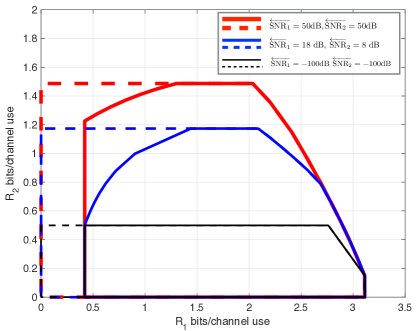
Figure 2: Achievable capacity regions $\underline{\mathcal{C}}$ (dashed-lines) in [4, Theorem $2$] and achievable $\eta$-NE regions ${\underline{\mathcal{N}}_{\eta}}$ (solid lines) in Theorem 1 of the two-user GIC-NOF and two-user D-GIC-NOF with parameters $\overrightarrow{\mathrm{SNR}}_{1}=24$ dB, $\overrightarrow{\mathrm{SNR}}_{2}=3$ dB, $\mathrm{INR}_{12}=16$ dB, $\mathrm{INR}_{21}=9$ dB, $\overleftarrow{\mathrm{SNR}}_{1}\in\{-100,18,50\}$ dB, $\overleftarrow{\mathrm{SNR}}_{2}\in\{-100,8,50\}$ dB and $\eta=1$.

The competitive interaction between the two transmitter-receiver pairs in the interference channel can be modeled by the following game in normal-form:

$$\mathcal{G}=\left(\mathcal{K},\left\{\mathcal{A}_{k}\right\}_{k\in\mathcal{K}},\left\{u_{k}\right\}_{k\in\mathcal{K}}\right).$$ (11)

The set $\mathcal{K}=\{1,2\}$ is the set of players, that is, the set of transmitter-receiver pairs. The sets $\mathcal{A}_{1}$ and $\mathcal{A}_{2}$ are the sets of actions of players $1$ and $2$, respectively. An action of a player $i\in\mathcal{K}$, which is denoted by $s_{i}\in\mathcal{A}_{i}$, is basically its transmit-receive configuration as described above. The utility function of player $i$ is $u_{i}:\mathcal{A}_{1}\times\mathcal{A}_{2}\rightarrow\mathds{R}_{+}$ and it is defined as the information rate of transmitter $i$,

$$u_{i}(s_{1},s_{2})=\left\{\begin{array}[]{lcl}R_{i},&\mbox{if}&p_{i}(s_{1},s_{2})<\epsilon\\ 0,&&\mbox{otherwise,}\end{array}\right.$$ (12)

where $\epsilon>0$ is an arbitrarily small number. This game formulation for the case without feedback was first proposed in [9] and [10].

A class of transmit-receive configurations that are particularly important in the analysis of this game is referred to as the set of $\eta$-Nash equilibria ($\eta$-NE), with $\eta>0$. This type of configurations satisfy the following definition.

Definition 2 ($\eta$-Nash equilibrium)

Given a positive real $\eta$, an action profile $(s_{1}^{*},s_{2}^{*})$ is an $\eta$-Nash equilibrium (NE) in the game ${\mathcal{G}=\left(\mathcal{K},\left\{\mathcal{A}_{k}\right\}_{k\in\mathcal{K}},\left\{u_{k}\right\}_{k\in\mathcal{K}}\right)}$, if for all $i\in\mathcal{K}$ and for all $s_{i}\in\mathcal{A}_{i}$, it follows that

$$u_{i}(s_{i},s_{j}^{*})\leqslant u_{i}(s_{i}^{*},s_{j}^{*})+\eta.$$ (13)

Let $(s_{1}^{*},s_{2}^{*})$ be an $\eta$-Nash equilibrium action profile. Then, none of the transmitters can increase its own transmission rate more than $\eta$ bits per channel use by changing its own transmit-receive configuration and keeping the average bit error probability arbitrarily close to zero. Note that for $\eta$ sufficiently large, from Definition 2, any pair of configurations can be an $\eta$-NE. Alternatively, for $\eta=0$, the definition of Nash equilibrium is obtained [11]. In this case, if a pair of configurations is a Nash equilibrium ($\eta=0$), then each individual configuration is optimal with respect to each other. Hence, the interest is to describe the set of all possible $\eta$-NE rate pairs $(R_{1},R_{2})$ of the game in (11) with the smallest $\eta$ for which there exists at least one equilibrium configuration pair.

The set of rate pairs that can be achieved at an $\eta$-NE is known as the $\eta$-Nash equilibrium ($\eta$-NE) region.

Definition 3 ($\eta$-NE Region)

Let $\eta>0$ be fixed. An achievable rate pair $(R_{1},R_{2})$ is said to be in the $\eta$-NE region of the game $\mathcal{G}=\left(\mathcal{K},\left\{\mathcal{A}_{k}\right\}_{k\in\mathcal{K}},\left\{u_{k}\right\}_{k\in\mathcal{K}}\right)$ if there exists a pair $(s_{1}^{*},s_{2}^{*})\in\mathcal{A}_{1}\times\mathcal{A}_{2}$ that is an $\eta$-NE and the following holds:

$$u_{1}(s_{1}^{*},s_{2}^{*})=R_{1} u_{2}(s_{1}^{*},s_{2}^{*})=R_{2}.$$ and (14)

The $\eta$-NE regions of the two-user GIC with and without perfect channel-output feedback have been approximated to within a constant number of bits in [5] and [6], respectively. The next section introduces a generalization of these results.

IV Main Results

IV-A Achievable $\eta$-Nash Equilibrium Region

Let the $\eta$-NE region (Definition 3) of the D-GIC-NOF be denoted by $\mathcal{N}_{\eta}$. This section introduces a region ${\underline{\mathcal{N}}_{\eta}}\subseteq\mathcal{N}_{\eta}$ that is achievable using a coding scheme that combines rate splitting [12], common randomness [5, 6], block Markov superposition coding [13] and backward decoding [14]. In the following, this coding scheme is referred to as randomized Han-Kobayashi scheme with noisy channel-output feedback (RHK-NOF). This coding scheme is presented in [8] and uses the same techniques of the schemes in [5] and [6]. Therefore, the focus of this section is on the results rather than the description of the scheme. A motivated reader is referred to [15]. The RHK-NOF is proved to be an $\eta$-NE action profile with $\eta\geqslant 1$. That is, any unilateral deviation from the RHK-NOF by any of the transmitter-receiver pairs might lead to an individual rate improvement which is at most one bit per channel use.

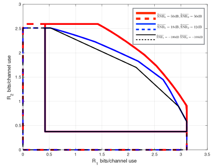
Figure 3: Achievable capacity regions $\underline{\mathcal{C}}$ (dashed-lines) in [4, Theorem $2$] and achievable $\eta$-NE regions ${\underline{\mathcal{N}}_{\eta}}$ (solid lines) in Theorem 1 of the two-user GIC-NOF and two-user D-GIC-NOF with parameters $\overrightarrow{\mathrm{SNR}}_{1}=24$ dB, ${\overrightarrow{\mathrm{SNR}}_{2}=18}$ dB, $\mathrm{INR}_{12}=16$ dB, $\mathrm{INR}_{21}=10$ dB, $\overleftarrow{\mathrm{SNR}}_{1}\in\{-100,18,50\}$ dB, $\overleftarrow{\mathrm{SNR}}_{2}\in\{-100,12,50\}$ dB and $\eta=1$.

The description of the achievable $\eta$-Nash region ${\underline{\mathcal{N}}_{\eta}}$ is presented using the constants $a_{1,i}$; the functions $a_{2,i}:[0,1]\rightarrow\mathds{R}_{+}$, $a_{l,i}:[0,1]^{2}\rightarrow\mathds{R}_{+}$, with $l\in\{3,\ldots,6\}$; and $a_{7,i}:[0,1]^{3}\rightarrow\mathds{R}_{+}$, which are defined as follows, for all $i\in\{1,2\}$, with $j\in\{1,2\}\setminus\{i\}$:

$$a_{1,i} = \frac{1}{2}\log\left(2+\frac{\overrightarrow{\mathrm{SNR}_{i}}}{\mathrm{INR}_{ji}}\right)-\frac{1}{2},$$ (15a)

$$a_{2,i}(\rho) = \frac{1}{2}\log\Big{(}b_{1,i}(\rho)+1\Big{)}-\frac{1}{2},$$ (15b)

$$a_{3,i}(\rho,\mu) = \!\frac{1}{2}\!\log\!\left(\!\frac{\!\overleftarrow{\mathrm{SNR}}_{i}\!\Big{(}b_{2,i}(\rho)+2\Big{)}+b_{1,i}(1)+1}{\overleftarrow{\mathrm{SNR}}_{i}\Big{(}\!\left(1\!-\!\mu\right)\!b_{2,i}(\rho)\!+\!2\Big{)}\!+\!b_{1,i}(1)\!+\!1}\!\right)\!,$$

$$a_{4,i}(\rho,\mu) = \frac{1}{2}\log\bigg{(}\Big{(}1-\mu\Big{)}b_{2,i}(\rho)+2\bigg{)}-\frac{1}{2},$$ (15d)

$$a_{5,i}(\rho,\mu) = \frac{1}{2}\log\left(2+\frac{\overrightarrow{\mathrm{SNR}}_{i}}{\mathrm{INR}_{ji}}+\Big{(}1-\mu\Big{)}b_{2,i}(\rho)\right)-\frac{1}{2},$$

$$a_{6,i}(\rho,\mu) = \frac{1}{2}\!\log\!\left(\!\frac{\overrightarrow{\mathrm{SNR}}_{i}}{\mathrm{INR}_{ji}}\bigg{(}\Big{(}1\!-\!\mu\Big{)}b_{2,j}(\rho)\!+\!1\bigg{)}\!+\!2\right)\!-\!\frac{1}{2},$$

$$a_{7,i}(\rho,\!\mu_{1}\!,\!\mu_{2}\!) = \frac{1}{2}\!\log\Bigg{(}\!\frac{\overrightarrow{\mathrm{SNR}}_{i}}{\mathrm{INR}_{ji}}\bigg{(}\Big{(}1\!-\!\mu_{i}\Big{)}b_{2,j}(\rho)\!+\!1\bigg{)}$$ (15f)

$$+\Big{(}1\!-\!\mu_{j}\Big{)}b_{2,i}(\rho)+2\Bigg{)}\!-\!\frac{1}{2},$$

where the functions $b_{l,i}:[0,1]\rightarrow\mathds{R}_{+}$, with $l\in\{1,2\}$ are defined as follows:

$$b_{1,i}(\rho) = \overrightarrow{\mathrm{SNR}}_{i}+2\rho\sqrt{\overrightarrow{\mathrm{SNR}}_{i}\mathrm{INR}_{ij}}+\mathrm{INR}_{ij}\mbox{ and }$$ (16a)

$$b_{2,i}(\rho) = \Big{(}1-\rho\Big{)}\mathrm{INR}_{ij}-1.$$ (16b)

Note that the functions in (15) and (16) depend on $\overrightarrow{\mathrm{SNR}}_{1}$, $\overrightarrow{\mathrm{SNR}}_{2}$, $\mathrm{INR}_{12}$, $\mathrm{INR}_{21}$, $\overleftarrow{\mathrm{SNR}}_{1}$, and $\overleftarrow{\mathrm{SNR}}_{2}$, however as these parameters are fixed in this analysis, this dependence is not emphasized in the definition of these functions. Finally, using this notation, the achievable $\eta$-NE region is presented by Theorem 1 on the next page. The proof of Theorem 1 is presented in [8]. The inequalities in (17) are additional conditions to those defining the region $\underline{\mathcal{C}}$ in [4, Theorem 2]. More specifically, the $\eta$-NE region is described by the intersection of the achievable region $\underline{\mathcal{C}}$ and the set of rate pairs $(R_{1},R_{2})$ satisfying (17).

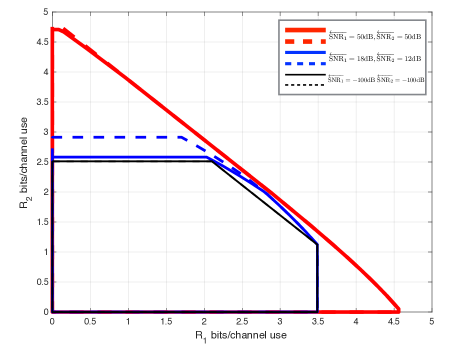
Figure 4: Achievable capacity regions $\underline{\mathcal{C}}$ (dashed-lines) in [4, Theorem $2$] and achievable $\eta$-NE regions ${\underline{\mathcal{N}}_{\eta}}$ (solid lines) in Theorem 1 of the two-user GIC-NOF and two-user D-GIC-NOF with parameters $\overrightarrow{\mathrm{SNR}}_{1}=24$ dB, ${\overrightarrow{\mathrm{SNR}}_{2}=18}$ dB, $\mathrm{INR}_{12}=48$ dB, $\mathrm{INR}_{21}=30$ dB, $\overleftarrow{\mathrm{SNR}}_{1}\in\{-100,18,50\}$ dB, $\overleftarrow{\mathrm{SNR}}_{2}\in\{-100,12,50\}$ dB and $\eta=1$.

Theorem 1

Let $\eta\geqslant 1$ be fixed. The achievable $\eta$-NE region ${\underline{\mathcal{N}}_{\eta}}$ is given by the closure of all possible achievable rate pairs $(R_{1},R_{2})\in\underline{\mathcal{C}}$ in [4, Theorem $2$] that satisfy, for all $i\in\{1,2\}$ and $j\in\{1,2\}\setminus\{i\}$, the following conditions:

$$R_{i} \geqslant \Big{(}a_{2,i}(\rho)-a_{3,i}(\rho,\mu_{j})-a_{4,i}(\rho,\mu_{j})-\eta\Big{)}^{+},$$ (17a)

$$R_{i} \leqslant \min\Big{(}a_{2,i}(\rho)+a_{3,j}(\rho,\mu_{i})+a_{5,j}(\rho,\mu_{i})-a_{2,j}(\rho)+\eta,$$

$$a_{3,i}(\rho,\mu_{j})+a_{7,i}(\rho,\mu_{1},\mu_{2})+2a_{3,j}(\rho,\mu_{i})+a_{5,j}(\rho,\mu_{i})-a_{2,j}(\rho)+\eta,$$

$$\!a_{2,i}(\rho)\!+\!a_{3,i}(\rho,\mu_{j})\!+\!2a_{3,j}(\rho,\mu_{i})\!+\!a_{5,j}(\rho,\mu_{i})\!+\!a_{7,j}(\rho,\mu_{1},\mu_{2})\!-\!2a_{2,j}(\rho)+2\eta\Big{)},$$

$$R_{1}+R_{2} \leqslant a_{1,i}\!+\!a_{3,i}(\rho,\mu_{j})\!+\!a_{7,i}(\rho,\mu_{1},\mu_{2})\!+\!a_{2,j}(\rho)\!+\!a_{3,j}(\rho,\mu_{1})\!-\!a_{2,i}(\rho)+\eta,$$ (17c)

for all $\left(\rho,\mu_{1},\mu_{2}\right)\in\left[0,\left(1-\max\left(\frac{1}{\mathrm{INR}_{12}},\frac{1}{\mathrm{INR}_{21}}\right)\right)^{+}\right]\times[0,1]\times[0,1]$.

 

Figure 2 shows the achievable region $\underline{\mathcal{C}}$ in [4, Theorem $2$] of a two-user centralized GIC-NOF and the achievable $\eta$-NE region ${\underline{\mathcal{N}}_{\eta}}$ in Theorem 1 of a two-user D-GIC-NOF with parameters $\overrightarrow{\mathrm{SNR}}_{1}=24$ dB, $\overrightarrow{\mathrm{SNR}}_{2}=3$ dB, $\mathrm{INR}_{12}=16$ dB, $\mathrm{INR}_{21}=9$ dB, $\overleftarrow{\mathrm{SNR}}_{1}\in\{-100,18,50\}$ dB, $\overleftarrow{\mathrm{SNR}}_{2}\in\{-100,8,50\}$ dB and $\eta=1$. Note that in this case, the feedback parameter $\overleftarrow{\mathrm{SNR}_{2}}$ does not have an effect on the achievable $\eta$-NE region ${\underline{\mathcal{N}}_{\eta}}$ and the achievable capacity region $\underline{\mathcal{C}}$ ([4, Theorem $2$]). This is due to the fact that when one transmitter-receiver pair is in low interference regime (LIR) and the other transmitter-receiver pair is in high interference regime (HIR), feedback is useless on the transmitter-receiver pair in HIR [15, 16].

Figure 3 shows the achievable region $\underline{\mathcal{C}}$ in [4, Theorem $2$] of a two-user centralized GIC-NOF and the achievable $\eta$-NE region ${\underline{\mathcal{N}}_{\eta}}$ in Theorem 1 of a two-user D-GIC-NOF with parameters $\overrightarrow{\mathrm{SNR}}_{1}=24$ dB, $\overrightarrow{\mathrm{SNR}}_{2}=18$ dB, $\mathrm{INR}_{12}=16$ dB, $\mathrm{INR}_{21}=10$ dB, $\overleftarrow{\mathrm{SNR}}_{1}\in\{-100,18,50\}$ dB, $\overleftarrow{\mathrm{SNR}}_{2}\in\{-100,12,50\}$ dB and $\eta=1$. Figure 4 shows the achievable region $\underline{\mathcal{C}}$ in [4, Theorem $2$] of a two-user centralized GIC-NOF and the achievable $\eta$-NE region ${\underline{\mathcal{N}}_{\eta}}$ in Theorem 1 of a two-user D-GIC-NOF with parameters $\overrightarrow{\mathrm{SNR}}_{1}=24$ dB, $\overrightarrow{\mathrm{SNR}}_{2}=18$ dB, $\mathrm{INR}_{12}=48$ dB, $\mathrm{INR}_{21}=30$ dB, $\overleftarrow{\mathrm{SNR}}_{1}\in\{-100,18,50\}$ dB, $\overleftarrow{\mathrm{SNR}}_{2}\in\{-100,12,50\}$ dB and $\eta=1$. In this case, the achievable $\eta$-NE region ${\underline{\mathcal{N}}_{\eta}}$ in Theorem 1 and achievable region $\underline{\mathcal{C}}$ on the capacity region [4, Theorem 2] are almost identical, which implies that in the cases in which $\overrightarrow{\mathrm{SNR}_{i}}<\mathrm{INR}_{ij}$, for both $i\in\{1,2\}$, with $j\in\{1,2\}\setminus\{i\}$, the achievable $\eta$-NE region is almost the same as the achievable capacity region in the centralized case studied in [4]. At low values of $\overleftarrow{\mathrm{SNR}}_{1}$ and $\overleftarrow{\mathrm{SNR}}_{2}$, the achievable $\eta$-NE region approaches the rectangular region reported in [5] for the case of the two-user decentralized GIC (D-GIC). Alternatively, for high values of $\overleftarrow{\mathrm{SNR}}_{1}$ and $\overleftarrow{\mathrm{SNR}}_{2}$, the achievable $\eta$-NE region approaches the region reported in [6] for the case of the two-user decentralized GIC with perfect channel-output feedback (D-GIC-POF). These observations are formalized by the following corollaries.

Denote by ${\underline{\mathcal{N}}_{\eta}}_{\mathrm{PF}}$ the achievable $\eta$-NE region of the two-user D-GIC-POF presented in [6]. The region ${\underline{\mathcal{N}}_{\eta}}_{\mathrm{PF}}$ can be obtained as a special case of Theorem 1 as shown by the following corollary.

Corollary 1 ($\eta$-NE Region with Perfect Output Feedback)

Let ${\underline{\mathcal{N}}_{\eta}}_{\mathrm{PF}}$ denote the achievable $\eta$-NE region of the two-user D-GIC-POF with fixed parameters $\overrightarrow{\mathrm{SNR}}_{i}$ and $\mathrm{INR}_{ij}$, with $i\in\{1,2\}$ and $j\in\{1,2\}\backslash\{i\}$. Then, the following holds:

$${\underline{\mathcal{N}}_{\eta}}_{\mathrm{PF}}=\lim_{\tiny\begin{array}[]{l}\overleftarrow{\mathrm{SNR}}_{1}\rightarrow\infty\\ \overleftarrow{\mathrm{SNR}}_{2}\rightarrow\infty\end{array}}{\underline{\mathcal{N}}_{\eta}}.$$ (20)

Denote by ${\underline{\mathcal{N}}_{\eta}}_{\mathrm{WF}}$ the achievable $\eta$-NE region of the two-user D-GIC presented in [5]. The region ${\underline{\mathcal{N}}_{\eta}}_{\mathrm{WF}}$ can be obtained as a special case of Theorem 1 as shown by the following corollary.

Corollary 2 ($\eta$-NE Region without Output Feedback )

Let ${\underline{\mathcal{N}}_{\eta}}_{\mathrm{WF}}$ denote the achievable $\eta$-NE region of the two-user D-GIC, with fixed parameters $\overrightarrow{\mathrm{SNR}}_{i}$ and $\mathrm{INR}_{ij}$, with $i\in\{1,2\}$ and $j\in\{1,2\}\backslash\{i\}$. Then, the following holds:

$${\underline{\mathcal{N}}_{\eta}}_{\mathrm{WF}}=\lim_{\tiny\begin{array}[]{r}\overleftarrow{\mathrm{SNR}}_{1}\rightarrow 0\\ \overleftarrow{\mathrm{SNR}}_{2}\rightarrow 0\\ \rho=0.\end{array}}{\underline{\mathcal{N}}_{\eta}}.$$ (24)

IV-B Imposibility Region

This section introduces an imposibility region, denoted by $\overline{\mathcal{N}}_{\eta}$. That is, $\overline{\mathcal{N}}_{\eta}\supseteq\mathcal{N}_{\eta}$. More specifically, any rate pair $\left(R_{1},R_{2}\right)\in\overline{\mathcal{N}}_{\eta}^{\mathsf{c}}$ is not an $\eta$-NE. This region is described in terms of the convex region $\overline{\mathcal{B}}_{\mathrm{G-IC-NOF}}$. Here, for the case of the two-user D-GIC-NOF, the region $\overline{\mathcal{B}}_{\mathrm{G-IC-NOF}}$ is given by the closure of the rate pairs $(R_{1},R_{2})\in\mathds{R}_{+}^{2}$ that satisfy for all $i\in\{1,2\}$, with $j\in\{1,2\}\setminus\{i\}$:

$$\overline{\mathcal{B}}_{\mathrm{G-IC-NOF}} = \Big{\{}(R_{1},R_{2})\in\mathds{R}_{+}^{2}:R_{i}\geqslant L_{i},$$ (25)

$$\mbox{ for all }i\in\mathcal{K}=\{1,2\}\Big{\}},$$

where,

$$L_{i} \triangleq \left(\frac{1}{2}\log\left(1+\frac{\overrightarrow{\mathrm{SNR}}_{i}}{1+\mathrm{INR}_{ij}}\right)-\eta\right)^{+}.$$ (26)

Note that $L_{i}$ is the rate achieved by the transmitter-receiver pair $i$ when it saturates the power constraint in (5) and treats interference as noise. Following this notation, the imposibility region of the two-user GIC-NOF, i.e., $\overline{\mathcal{N}}_{\eta}$, can be described as follows.

Theorem 2

Let $\eta\geqslant 1$ be fixed. The imposibility region $\overline{\mathcal{N}}_{\eta}$ of the two-user D-GIC-NOF is given by the closure of all possible non-negative rate pairs $(R_{1},R_{2})\in\overline{\mathcal{C}}\cap\overline{\mathcal{B}}_{\mathrm{G-IC-NOF}}$ for all $\rho\in[0,1]$.

The impossibility region in Theorem 2 has been first presented in [6] and it is very loose in this case. A better impossibility region is presented in [15].

V Conclusions

In this paper, an achievable $\eta$-Nash equilibrium ($\eta$-NE) region for the two-user Gaussian interference channel with noisy channel-output feedback has been presented for all $\eta\geqslant 1$. This result generalizes the existing achievable regions of the $\eta$-NE for the the cases without feedback and with perfect channel-output feedback.

References

- [1] R. H. Etkin, D. N. C. Tse, and W. Hua, “Gaussian interference channel capacity to within one bit,” IEEE Trans. Inf. Theory, vol. 54, no. 12, pp. 5534–5562, Dec. 2008.
- [2] C. Suh and D. N. C. Tse, “Feedback capacity of the Gaussian interference channel to within 2 bits,” IEEE Trans. Inf. Theory, vol. 57, no. 5, pp. 2667–2685, May. 2011.
- [3] S.-Q. Le, R. Tandon, M. Motani, and H. V. Poor, “Approximate capacity region for the symmetric Gaussian interference channel with noisy feedback,” IEEE Trans. Inf. Theory, vol. 61, no. 7, pp. 3737–3762, Jul. 2015.
- [4] V. Quintero, S. M. Perlaza, I. Esnaola, and J.-M. Gorce, “Approximate capacity region of the two-user Gaussian interference channel with noisy channel-output feedback,” IEEE Trans. Inf. Theory, vol. 64, no. 7, pp. 5326–5358, Jul 2018.
- [5] R. A. Berry and D. N. C. Tse, “Shannon meets Nash on the interference channel,” IEEE Trans. Inf. Theory, vol. 57, no. 5, pp. 2821–2836, May. 2011.
- [6] S. M. Perlaza, R. Tandon, H. V. Poor, and Z. Han, “Perfect output feedback in the two-user decentralized interference channel,” IEEE Trans. Inf. Theory, vol. 61, no. 10, pp. 5441–5462, Oct. 2015.
- [7] V. Quintero, S. M. Perlaza, J.-M. Gorce, and H. V. Poor, “Nash region of the linear deterministic interference channel with noisy output feedback,” in Proc. IEEE Int. Symp. on Inform. Theory (ISIT), Aachen, Germany, Jun. 2017.
- [8] ——, “Decentralized interference channels with noisy output feedback,” INRIA, Lyon, France, Tech. Rep. 9011, Jan. 2017.
- [9] R. D. Yates, D. Tse, and Z. Li, “Secret communication on interference channels,” in Proc. IEEE International Symposium on Information Theory (ISIT), Toronto, Canada, Jul. 2008.
- [10] R. Berry and D. N. C. Tse, “Information theoretic games on interference channels,” in Proc. IEEE International Symposium on Information Theory (ISIT), Toronto,Canada, Jul. 2008.
- [11] J. F. Nash, “Equilibrium points in -person games,” Proc. National Academy of Sciences of the United States of America, vol. 36, no. 1, pp. 48–49, Jan. 1950.
- [12] T. S. Han and K. Kobayashi, “A new achievable rate region for the interference channel,” IEEE Trans. Inf. Theory, vol. 27, no. 1, pp. 49–60, Jan. 1981.
- [13] T. M. Cover and C. S. K. Leung, “An achievable rate region for the multiple-access channel with feedback,” IEEE Trans. Inf. Theory, vol. 27, no. 3, pp. 292–298, May. 1981.
- [14] F. M. J. Willems, “Information theoretical results for multiple access channels,” Ph.D. dissertation, Katholieke Universiteit, Leuven, Belgium, Oct. 1982.
- [15] V. Quintero, “Noisy channel-output feedback in the interference channel,” Ph.D. dissertation, Université de Lyon, Lyon, France., Dec. 2017.
- [16] V. Quintero, S. M. Perlaza, I. Esnaola, and J.-M. Gorce, “When does output feedback enlarge the capacity of the interference channel?” IEEE Trans. Commun., vol. 66, no. 2, pp. 615–628, Feb. 2018.