Astrophysical S-factors, thermonuclear rates, and electron screening potential for the ³He(d,p)⁴He Big Bang reaction via a hierarchical Bayesian model

Abstract

We developed a hierarchical Bayesian framework to estimate S-factors and thermonuclear rates for the ³He(d,p)⁴He reaction, which impacts the primordial abundances of ³He and ⁷Li. The available data are evaluated and all direct measurements are taken into account in our analysis for which we can estimate separate uncertainties for systematic and statistical effects. For the nuclear reaction model, we adopt a single-level, two-channel approximation of R-matrix theory, suitably modified to take the effects of electron screening at lower energies into account. In addition to the usual resonance parameters (resonance location and reduced widths for the incoming and outgoing reaction channel), we include the channel radii and boundary condition parameters in the fitting process. Our new analysis of the ³He(d,p)⁴He S-factor data results in improved estimates for the thermonuclear rates. This work represents the first nuclear rate evaluation using R-matrix theory embedded into a hierarchical Bayesian framework, properly accounting for all known sources of uncertainty. Therefore, it provides a test bed for future studies of more complex reactions.

1 Introduction

The big-bang theory rests on three observational pillars: big-bang nucleosynthesis (BBN; Gamow, 1948; Cyburt et al., 2016), the cosmic expansion (Riess et al., 1998; Peebles & Ratra, 2003), and the cosmic microwave background radiation (Spergel et al., 2007; Planck Collaboration et al., 2016). The BBN takes place during the first 20 minutes after the big bang, at temperatures and densities near $1$ GK and 10^-5 g/cm³, and is responsible for the production of the lightest nuclides, which play a major role in the subsequent history of cosmic evolution.

Primordial nucleosynthesis provides a sensitive test of the big bang model if the uncertainties in the predicted abundances can be reduced to the level of the uncertainties in the observed abundances. The uncertainties for the observed primordial abundances of ⁴He, ²H (or D), and ⁷Li have been greatly reduced in recent years and amount to 1.6%, 1.2%, and 20%, respectively (Aver et al., 2015; Cooke et al., 2018; Sbordone et al., 2010). For the observed primordial ³He abundance, only an upper limit is available (³He/H $\leq$ $1.3\times 10^{-5}$; Bania et al. 2002). At present, the uncertainties in the predicted abundances of ⁴He, ²H (or D), ³He, and ⁷Li amount to 0.07%, 1.5%, 2.4%, and 4.4%, respectively (Pitrou et al., 2018). The primordial abundances predicted by the big bang model are in reasonable agreement with observations, as shown in Figure 1, except for the ⁷Li/H ratio, where the predicted value (Cyburt et al., 2016) exceeds the observed one (Sbordone et al., 2010) by a factor of $\approx$ $3$. This long-standing “lithium problem” has not found a satisfactory solution yet (see e.g., Cyburt et al., 2016, for a review).

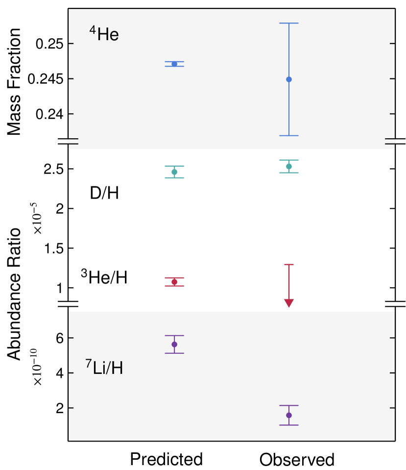
Figure 1: Predicted (left) versus observed (right) primordial abundances for the light nuclei: ⁴He, D, ³He and ⁷Li. For ⁴He the mass fraction is shown, while for the other species the number abundance ratios relative to hydrogen are displayed. The uncertainties representing 95% coverage intervals for the predicted abundances are from Pitrou et al. (2018), while the observed abundances are obtained from Aver et al. (2015) (⁴He), Cooke et al. (2018) (D), and Sbordone et al. (2010) (⁷Li). For the observed primordial ³He abundance, only an upper limit is available (Bania et al., 2002), which we depict by a vertical arrow.

Twelve nuclear processes of interest take place during big bang nucleosynthesis, as illustrated in Figure 2. Among these are the weak interactions that transform neutrons into protons, and vice versa, and the p(n,$\gamma$)d reaction whose cross section can be calculated precisely using effective field theories (Savage et al., 1999; Ando et al., 2006). The ten remaining reactions, d(p,$\gamma$)³He, d(d,n)³He, d(d,p)t, t(d,n)⁴He, t($\alpha$,$\gamma$)⁷Li, ³He(d,p)⁴He, ³He(n,p)t, ³He($\alpha$,$\gamma$)⁷Be, ⁷Li(p,$\alpha$)⁴He, and ⁷Be(n,p)⁷Li, have been measured directly in the laboratory at the energies of astrophysical interest. Nevertheless, the estimation of thermonuclear reaction rates from the measured cross section (or S-factor) data remains challenging. Results obtained using $\chi^{2}$ optimization are plagued by a number of problems, including the treatment of systematic uncertainties, and the implicit assumption of normal likelihoods (see e.g., Andrae et al., 2010). Therefore, we have started an effort to derive statistically sound BBN reaction rates using a hierarchical Bayesian model. Bayesian rates have recently been derived for d(p,$\gamma$)³He, ³He($\alpha$,$\gamma$)⁷Be (Iliadis et al., 2016), d(d,n)³He, and d(d,p)³H (Gómez Iñesta et al., 2017). These studies adopted the cross section energy dependence from the microscopic theory of nuclear reactions, while the absolute cross section normalization was found from a fit to the data within the Bayesian framework.

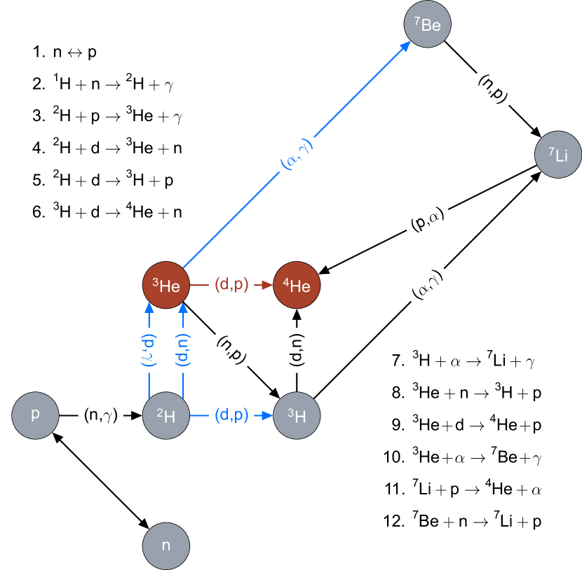
Figure 2: Nuclear reactions important for big bang nucleosynthesis. Reactions for which the rates have been obtained previously using Bayesian models are shown as blue arrows. The ³He(d,p)⁴He reaction, which is subject of the present work, is shown in red.

We report here the Bayesian reaction rates for a fifth big bang reaction, ³He(d,p)⁴He. This reaction marginally impacts the primordial deuterium abundance, but sensitively influences the primordial abundances of ³He and ⁷Li. For example, a reaction rate uncertainty of 5% at big bang temperatures translates to a 4% variation in the predicted abundance of both ³He and ⁷Li (Coc & Vangioni, 2010). Because of its low abundance, ³He has not been observed yet outside of our Galaxy. However, the next generation of large telescope facilities will likely enable the determination of the ³He/⁴He ratio from observations of extragalactic metal-poor Hii regions (Cooke, 2015). Therefore, although a revised ³He(d,p)⁴He reaction rate will not solve the ⁷Li problem, a more reliable rate is nevertheless desirable for improving the predicted BBN abundances.

The ³He(d,p)⁴He reaction has been studied extensively during the past few decades, not only because of its importance to BBN, but also because of its relevance to the understanding of the electron screening effect (e.g., Barker, 2007). At the lowest energies, the measured astrophysical S-factor shows a marked increase caused by electron screening effects. The data at those energies were used to derive the electron screening potential, but the results depended strongly on the data sets analyzed and the nuclear model applied.

To enable a robust treatment of different sources of uncertainties, we first evaluate the available cross section data and take only those experiments into account for which we can quantify the separate contributions of statistical and systematic effects to the total uncertainty. This leaves us with seven data sets to be analyzed. For the underlying nuclear model we assume a single-level, two-channel approximation of R-matrix theory (Descouvemont & Baye, 2010). As will be discussed below, we include both the channel radii and boundary conditions as fit parameters into the statistical model. This has not been done in most R-matrix studies because of the difficulty of obtaining acceptable fits via $\chi^{2}$ minimization. We will demonstrate that these parameters can be included naturally in our hierarchical Bayesian model. Compared to previous works (Iliadis et al., 2016; Gómez Iñesta et al., 2017), the present Bayesian model is more sophisticated and, therefore, represents an important test bed for future studies of more complex systems.

In Section 2, we summarize the reaction formalism. Our Bayesian model is discussed in Section 3, including likelihoods, model parameters, and priors. In Section 4, we present Bayesian S-factors and screening potentials. The thermonuclear reaction rates are presented in Section 5. A summary and conclusions are given in Section 6. Details about our data evaluation are provided in Appendix A.

2 Reaction Formalism

The ³He $+$ $d$ low-energy cross section is dominated by a s-wave resonance with a spin-parity of J^π $=$ $3/2^{+}$, corresponding to the second excited level near E_x $=$ $17$ MeV excitation energy in the ⁵Li compound nucleus (Tilley et al., 2002). This level decays via emission of d-wave protons. It has mainly a ³He $+$ $d$ structure, corresponding to a large deuteron spectroscopic factor (Barker, 1997).

Cross section (or S-factor) data for the ³He(d,p)⁴He reaction have been fitted in the past using various assumptions, including polynomials (Krauss et al., 1987), a Padé expansion (Barbui et al., 2013), R-matrix expressions (Barker, 2007), and hybrid models (Prati et al., 1994). Since we are mostly interested in the low-energy region, where the s-wave contribution dominates the cross section, we follow Barker (1997) and describe the theoretical energy dependence of the cross section (or S-factor) using a one-level, two-channel R-matrix approximation, suitably modified to take electron screening at low energies into account.

The inclusion of higher-lying levels and background poles in the formalism will likely not impact our results significantly. Hale et al. (2014) show (see their Fig. 4) that in the analog ³H(d,n)⁴He reaction the deviation in S-factors between a multi-level, multi-channel R-matrix fit and a single level R-matrix fit is less than 1.5% over the majority of the energy range shown. This deviation should be regarded as a worst case scenario, because the channel radii for these two fits were not the same.

In the one-level, two-channel R-matrix approximation, the integrated cross section of the ³He(d,p)⁴He reaction is given by

$$\sigma_{dp}(E)=\frac{\pi}{k_{d}^{2}}\frac{2J+1}{(2j_{1}+1)(2j_{2}+1)}\left|S_{dp}\right|^{2},$$ (1)

where $k_{d}$ and $E$ are the deuteron wave number and center-of-mass energy, respectively, J = 3/2 is the resonance spin, $j_{1}$ = 1/2 and $j_{2}$ = 1 are the ground-state spins of ³He and deuteron, respectively, and $S_{dp}$ is the scattering matrix element. The corresponding bare nucleus astrophysical S-factor of the ³He(d,p)⁴He reaction, which is not affected by electron screening, is given by

$$S_{bare}(E)=Ee^{2\pi\eta}\sigma_{dp}(E),$$ (2)

where $\eta$ is the Sommerfeld parameter. The scattering matrix element (Lane & Thomas, 1958) can be expressed as:

$$\left|S_{dp}\right|^{2}=\frac{\Gamma_{d}\Gamma_{p}}{(E_{0}+\Delta-E)^{2}+(\Gamma/2)^{2}},$$ (3)

where $E_{0}$ represents the level eigenenergy. The partial widths of the ³He $+$ d and ⁴He $+$ p channels ($\Gamma_{d}$, $\Gamma_{p}$), the total width ($\Gamma$), and the level shift ($\Delta$) are given by

$$\Gamma=\sum_{c}\Gamma_{c}~{},~{}~{}~{}\Gamma_{c}=2\gamma_{c}^{2}P_{c},$$ (4)

$$\Delta=\sum_{c}\Delta_{c}~{},~{}~{}~{}\Delta_{c}=-\gamma_{c}^{2}(S_{c}-B_{c}),$$ (5)

where $\gamma_{c}^{2}$ is the reduced width, and $B_{c}$ is the boundary condition parameter. Notice that we are not using the Thomas approximation (Thomas, 1951). Therefore, our partial and reduced widths are “formal” R-matrix parameters. Use of the Thomas approximation necessitates the definition of “observed” R-matrix parameters, which has led to significant confusion in the literature.

The energy-dependent quantities $P_{c}$ and $S_{c}$ denote the penetration factor and shift factors, respectively, for channel $c$ (either d $+$ ³He or p $+$ ⁴He), which are computed from the Coulomb wave functions, $F_{l}$ and $G_{l}$, according to:

$$P_{c}=\frac{k_{d}a_{c}}{F_{\ell}^{2}+G_{\ell}^{2}},\qquad S_{c}=\frac{k_{d}a_{c}(F_{\ell}F_{\ell}^{\prime}+G_{\ell}G_{\ell}^{\prime})}{F_{\ell}^{2}+G_{\ell}^{2}}.$$ (6)

The Coulomb wave functions and their derivatives are evaluated at the channel radius, $a_{c}$; the orbital angular momentum for a given channel is denoted by $\ell$.

The R-matrix channel radius is usually expressed as:

$$a_{c}=r_{0}\left(A_{1}^{1/3}+A_{2}^{1/3}\right),$$ (7)

where $A_{1}$ and $A_{2}$ are the mass numbers of the two interacting nuclei; $r_{0}$ denotes the radius parameter, with a value customarily chosen between $1$ fm and $2$ fm. Fitted R-matrix parameters and cross sections have a well-known dependence on the channel radii (see, e.g., deBoer et al., 2017), which arises from the truncation of the R-matrix to a restricted number of poles (i.e., a finite set of eigenenergies). The radius of a given channel has no rigorous physical meaning, except that the chosen values should exceed the sum of the radii of the colliding nuclei (e.g., Descouvemont & Baye, 2010). For the ³He(d,p)⁴He reaction, previous choices for the channel radii ranged between $3$ fm and $6$ fm (e.g., Barker, 2002; Descouvemont et al., 2004). In Section 4, we will discuss the impact of the channel radii on our derived S-factors by including them as parameters in our Bayesian model. This method ensures that correlations between model parameters are fully taken into account, contrary to the previously applied procedure of performing fits with two different, but fixed values of a channel radius. Notice that a few previous works have also treated the channel radii as fit parameters in their R-matrix analysis (e.g., Woods et al., 1988; Hale et al., 2014).

The energy, $E_{0}$, entering Equation 3 is the energy eigenvalue, and is not necessarily equal to the “energy at the center of the resonance” (Lane & Thomas, 1958). For a relatively narrow resonance, the scattering matrix element (and the S-factor and the cross section) peaks at the energy where the first term in the denominator of Equation 3 is equal to zero. Therefore, the resonance energy, $E_{r}$, is frequently defined as:

$$E_{0}+\Delta(E_{r})-E_{r}=0.$$ (8)

The boundary condition parameter is then chosen as:

$$B_{c}=S_{c}(E_{r}),$$ (9)

so that the level shift becomes zero at the center of the resonance. This assumption, which corresponds to setting the eigenenergy equal to the resonance energy ($E_{r}$ $=$ $E_{0}$), has also been adopted in most previous studies of the ³He(d,p)⁴He reaction (e.g., Barker, 2007). Notice, however, that for broad resonances this procedure predicts values of $E_{r}$ that do not coincide with the S-factor maximum anymore. This can be seen by comparing in Barker’s Table I the fitted values of $E_{r}$ (between 307 keV and 427 keV) with the measured energies of the S-factor peak, $E_{m}$ (between 200 keV and 241 keV, depending on the analyzed data set). In fact, the low-energy resonance in the ³He(d,p)⁴He reaction is so broad that the scattering matrix element, the cross section, and the S-factor peak at different energies, and, therefore, the definition of an “energy at the center of the resonance” becomes ambiguous.

The assumption of $E_{r}$ $=$ $E_{0}$ made in previous studies of the ³He(d,p)⁴He reaction fixes the boundary condition parameters and thereby reduces the number of fitting parameters. However, as its name implies, the boundary condition parameter represents a model parameter and it is our intention to include it in the fitting. We believe that previous studies did neither include the channel radii nor the boundary condition parameters in the fitting because of the difficulty to achieve acceptable $\chi^{2}$ fits. We will demonstrate below that acceptable fits can indeed be obtained using a hierarchical Bayesian model.

In this work, instead of providing the boundary condition parameters, $B_{c}$, directly, we find it more useful to report the equivalent results for the energy, $E_{B}$, at which the level shift is zero according to $B_{c}$ $=$ $S_{c}(E_{r})$ (see Equation 5). We use the notation $E_{B}$ instead of $E_{r}$ to emphasize that the value of $E_{B}$ does not correspond to any measured “resonance energy,” since such a quantity cannot be determined unambiguously for a broad resonance.

In laboratory experiments, electrons are usually bound to the interacting projectile and target nuclei. These electron clouds effectively reduce the Coulomb barrier and give rise to an increasing transmission probability. We perform the S-factor fit to the data using the expression (Assenbaum et al., 1987; Engstler et al., 1988):

$$S(E)\approx S_{bare}(E)e^{\pi\eta(U_{e}/E)},$$ (10)

where $U_{e}$ is the energy-independent electron screening potential.

Notice that the measurement can be performed in two ways, depending on the identity of the projectile and target. The situation is shown in Figure 3. The notation ³He(d,p)⁴He refers to a deuterium ion beam (without atomic electrons) directed onto a neutral ³He target, while d(³He,p)⁴He refers to a ³He ion beam directed onto a neutral deuterium target. These two situations result in different electron screening potentials, $U_{e}$. The distinction is particularly important at center-of-mass energies below $50$ keV, as will be shown below.

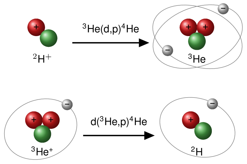
Figure 3: Illustration of the different configurations involved in the ³He(d,p)⁴He and d(³He,p)⁴He reactions. Top: deuterium ion beam (with no atomic electron) incident on a neutral ³He target atom. Bottom: ³He ion (with one atomic electron) incident on a neutral deuterium target atom. The electron screening effect is of different magnitude in these two situations.

3 Bayesian Model

3.1 General aspects

Bayesian probability theory provides a mathematical framework to infer, from the measured data, the degree of plausibility of model parameters (Jaynes & Bretthorst, 2003). It allows to update a current state of knowledge about a set of model parameters, $\theta$, in view of newly available information. The updated state of knowledge about $\theta$ is described by the posterior distribution, $p(\theta|y)$, i.e., the probability of the parameters, $\theta$, given the data, $y$. At the foundation of the theory lies Bayes’ theorem:

$$p(\theta|y)=\frac{\mathcal{L}(y|\theta)\pi(\theta)}{\int\mathcal{L}(y|\theta)\pi(\theta)d\theta}.$$ (11)

The numerator on the right side of Equation 11 represents the product of the model likelihood, $\mathcal{L}(y|\theta)$, i.e., the probability that the data, $y$, were obtained given the model parameters, $\theta$, and the prior distribution, $\pi(\theta)$, which represents our state of knowledge before considering the new data. The normalization factor appearing in the denominator, called the evidence, describes the probability of obtaining the data considering all possible parameter values.

In the Bayesian framework, the concept of hierarchical Bayesian models is of particular interest when accounting for different effects and processes that impact the measured data (Parent & Rivot, 2012; de Souza et al., 2015, 2016; Hilbe et al., 2017; González-Gaitán et al., 2019). The underlying idea is to decompose higher-dimensional problems into a number of probabilistically linked lower-dimensional substructures. Hierarchical Bayesian models allow for a consistent inclusion of different types of uncertainties into the model, thereby solving inferential problems that are not amenable to traditional statistics (e.g., Gelman & Hill, 2006; Parent & Rivot, 2012; Loredo, 2013; Long & de Souza, 2018).

3.2 Likelihoods and priors

We will next discuss how to construct likelihoods to quantify the different layers of uncertainty affecting the ³He(d,p)⁴He and d(³He,p)⁴He data, namely extrinsic scatter, statistical effects, and systematic effects.

Throughout this work, we evaluate the Bayesian models using an adaptive Markov Chain Monte-Carlo (MCMC) sampler called Differential Evolution MCMC with snooker update (ter Braak & Vrugt, 2008). The method exploits different sub-chain trajectories in parallel to optimally explore the multidimensional parameter space. The model was implemented using the general purpose MCMC sampler BayesianTools (Hartig et al., 2018) within the R language (Team R Development Core, 2010). Computing a Bayesian model refers to generating random samples from the posterior distribution of model parameters. This involves the definition of the model, likelihood, and priors, as well as the initialization, adaptation, and monitoring of the Markov chain. We evaluated the theoretical S-factor model for the ³He(d,p)⁴He reaction based on the R-matrix formalism (Section 2), including the effect of electron screening.

3.2.1 Extrinsic scatter

We will first discuss the treatment of the statistical uncertainties with unknown variance, which we will call extrinsic scatter. This extra variance encodes any additional sources of random uncertainty that were not properly accounted for by the experimenter. Suppose an experimental S-factor, $S_{exp}$, is free of systematic and statistical measurement uncertainties ($\epsilon_{syst}=0$, and $\epsilon_{stat}=0$), but is subject to an unknown additional scatter ($\epsilon_{extr}\neq 0$). If the variable under study is continuous, one can assume in the simplest case a Gaussian noise, with standard deviation of $\sigma_{extr}$. The model likelihood connecting experiment with theory, assuming a vector of model parameters, $\theta$, is then given by:

$$\mathcal{L}(S_{exp}|\theta)=\prod_{i=1}^{N}\frac{1}{\sqrt{2\pi\sigma_{extr}^{2}}}\exp\left[-\frac{(S_{exp;i}-S_{i}(\theta))^{2}}{2\sigma_{extr}^{2}}\right],$$ (12)

where $S_{i}(\theta)$ is the model S-factor (obtained from R-matrix theory), while the product runs over all data points, $N$, labeled by $i$. In symbolic notation, this expression can be written as:

$$S_{exp;i}\sim\mathrm{Normal}(S_{i}(\theta),\sigma_{extr}^{2}),$$ (13)

implying that the experimental S-factor datum, $i$, is sampled from a normal distribution, with a mean equal to the true value, $S_{i}(\theta)$, and a variance of $\sigma_{extr}^{2}$.

3.2.2 Statistical effects

Any experiment is subject to measurement uncertainties, which are the consequence of the randomness of the data-taking process. Suppose the measurement uncertainties are solely given by statistical effects of known variance, which differs for each data point of a given experiment (also known as heteroscedasticity), and that the likelihood can be described, in the simplest case, by a normal probability density. The likelihood for such model can be written as:

$$S_{exp;i}\sim\mathrm{Normal}(S_{i}(\theta),\sigma_{stat;i}^{2}),$$ (14)

where $\sigma^{2}_{stat;i}$ represents the variance of the normal density for datum $i$. Statistical uncertainties can be reduced by improving the data collection procedure.

When both statistical uncertainties, with known variance, and extrinsic scatter, with unknown variance, are present, the model can be easily extended to accommodate both effects. The likelihood for such a model is given by the nested expressions:

$$S^{\prime}_{i}\sim\mathrm{Normal}(S_{i}(\theta),\sigma_{extr}^{2}),$$ (15)

$$S_{exp;i}\sim\mathrm{Normal}(S^{\prime}_{i},\sigma_{stat;i}^{2}).$$ (16)

These expressions provide an intuitive view of how a chain of probabilistic disturbances can be combined into a hierarchical structure. First, a homoscedastic scatter, quantified by the standard deviation $\sigma_{extr}$ of a normal probability density, perturbs the theoretical value of a given S-factor datum, $S_{i}(\theta)$, to produce a value of $S^{\prime}_{i}$; second, the latter value is in turn perturbed by the heteroscedastic statistical uncertainty, quantified by the standard deviation $\sigma_{stat;i}$ of a normal probability density, to produce the measured value $S_{exp;i}$. The above demonstrates how an effect impacting the data can be implemented in a straightforward manner into a Bayesian data analysis.

3.2.3 Systematic effects

Systematic uncertainties are usually not reduced by combining the results from different measurements or by collecting more data. Reported systematic uncertainties are based on assumptions made by the experimenter, are model-dependent, and follow vaguely known probability distributions (Heinrich & Lyons, 2007). In a nuclear counting experiment, systematic effects impact the overall normalization by shifting all points of a given data set into the same direction, and they are often quantified by a multiplicative factor.

A useful distribution for normalization factors is the lognormal probability density:

$$f(x)=\frac{1}{\sigma_{L}x\sqrt{2\pi}}\exp\left[-\frac{(\ln x-\mu_{L})^{2}}{2\sigma_{L}^{2}}\right],$$ (17)

which is characterized by two quantities, the location parameter, $\mu_{L}$, and the shape parameter, $\sigma_{L}$. The median value of the lognormal distribution is given by $e^{\mu_{L}}$, while the factor uncertainty, $f.u.$, for a coverage probability of 68%, is $e^{\sigma_{L}}$. For example, if the systematic uncertainty for a given data set is reported as $\pm$ 10%, then $f.u.$ amounts to $1.10$. In our model, we include a systematic effect as an informative lognormal prior with a median of $1.0$, i.e., $\mu_{L}=0$, and $f.u.$ estimated from the systematic uncertainty.

In our model, we can include systematic uncertainties using the nested expressions:

$$S^{\prime}_{i}\sim\mathrm{Normal}(S_{i}(\theta),\sigma_{extr}^{2}),$$ (18)

$$S_{exp;i,j}\sim\mathrm{Normal}(\xi_{j}S^{\prime}_{i},\sigma_{stat;i}^{2}),$$ (19)

where $\xi_{j}$ denotes the normalization factor for data set $j$, which is drawn from a lognormal distribution.

3.2.4 Priors

Our choices of priors are summarized in Table 1. Previous estimates of the deuteron reduced width are of order $\approx 1.0$ MeV (Coc et al., 2012), which corresponds to values close to the Wigner limit (WL; Wigner & Eisenbud, 1947; Dover et al., 1969). We use a broad prior for the reduced widths, which is restricted to positive energies only, i.e., truncated normal distributions (TruncNormal) with a zero mean and standard deviation given by the Wigner limit $\gamma^{2}_{\rm WL}\equiv\hbar/(\mu_{c}a_{c}^{2})$, where $\mu_{c}$ is the reduced mass of the interacting pair of particles in channel $c$, and $\hbar$ is the reduced Planck constant.

Lane & Thomas (1958), recommend to chose the boundary condition, $B_{c}$, in the one-level approximation so that the eigenvalue $E_{0}$ lies within the width of the observed resonance. Thus we chose for $E_{0}$ a uniform prior between 0.1 and 0.4 MeV. For the energy, $E_{B}$, at which the level shift is zero according to Equations 5 and 9, we chose a broad TruncNormal prior with zero mean, and a standard deviation of 1.0 MeV.

Woods et al. (1988) performed an R-matrix fit of experimental line shapes in the ⁴He(⁷Li,⁶Li)⁵He and ⁴He(⁷Li,⁶He)⁵Li stripping reactions and reported a best-fit value, for the channel radii, of 5.5 $\pm$ 1.0 fm for the ⁵He system. We then adopt for the channel radii uniform priors in the range of $2.0$ $-$ $10.0$ fm.

As for the electron screening potential, Aliotta et al. (2001) obtained values of $U_{e}$ $=$ $146\pm 5$ eV for the d(³He,p)⁴He reaction, and $U_{e}$ $=$ $201\pm 10$ eV for the ³He(d,p)⁴He reaction. For $U_{e}$, we will adopt a weakly informative prior given by a TruncNormal distribution with zero mean, and a standard deviation of 100 keV for both scenarios.

As already pointed out above, lognormal priors are adopted for the normalization factors, $\xi_{j}$, of each experiment, $j$. For a given systematic uncertainty $\sigma_{syst}$, the factor uncertainty, $f.u.$, is given by 1 + $\sigma_{syst}$, so if $\sigma_{syst}=2.5\%$, then $f.u.=1.025$. For a coverage probability of 68%, we have $f.u.=e^{\sigma_{L}}$. The priors are then given by:

$$\xi_{j}\sim\mathrm{LogNormal}(0,\ln^{2}(f.u._{j})),$$ (20)

where $f.u._{j}$ denotes the factor uncertainty for experiment $j$. Finally, for the extrinsic scatter, we employed a broad TruncNormal distribution with zero mean, and a standard deviation of 5 MeV b.

Table 1: Prior choices.

Parameter	Prior
$E_{0}$	Uniform(0.1, 0.4)
$E_{B}$	TruncNormal(0, $1.0^{2}$)
$\gamma_{d}^{2}$	TruncNormal(0, $(\gamma^{2}_{\rm WL,d})^{2}$)
$\gamma_{p}^{2}$	TruncNormal(0, $(\gamma^{2}_{\rm WL,p})^{2}$)
$a_{d}$	Uniform(2.0, 10.0)
$a_{p}$	Uniform(2.0, 10.0)
$U_{e}$	TruncNormal(0, $0.1^{2}$)
$\sigma_{extr}$	TruncNormal($0,5^{2}$)
$\xi$	LogNormal($0,\sigma_{L}^{2}$)

4 Analysis of ³He(d,p)⁴He

The current status of the available data for the ³He(d,p)⁴He and d(³He,p)⁴He reactions is discussed in detail in Appendix A. For the present analysis, we adopt the results of Zhichang et al. (1977); Krauss et al. (1987); Möller & Besenbacher (1980); Geist et al. (1999); Costantini et al. (2000); Aliotta et al. (2001), because only these data sets allow for a separate estimation of statistical and systematic uncertainties. In total, our compilation includes $214$ data points at center-of-mass energies between $4.2$ keV and $471$ keV.

4.1 Results

Our model contains $16$ parameters: six R-matrix parameters, seven normalization factors ($\xi_{1},\ldots,\xi_{7}$), the extrinsic scatter ($\sigma_{extr}$), and the two screening potentials (U_e1,U_e2) for the ³He(d,p)⁴He and d(³He,p)⁴He reactions, respectively. The full hierarchical Bayesian model can be summarized as:

$$\rm{Likelihood:}$$

$$\indent S^{\prime}_{i}\sim\mathrm{Normal}(S_{i}(\theta)e^{\pi\eta(U_{ek}/E_{exp;i})},\sigma_{extr}^{2}),$$

$$\indent S_{exp;i,j}\sim\mathrm{Normal}(\xi_{j}S^{\prime}_{i},\sigma_{stat;i}^{2}).$$

$$\mathrm{R{\text{-}}matrix~{}Parameters:}$$

$$\indent\theta\equiv(E_{0},E_{B},\gamma_{d}^{2},\gamma_{p}^{2},a_{d},a_{p}).$$

$$\rm{Priors:}$$ (21)

$$\indent E_{0}\sim\rm{Uniform}(0.1,0.4),$$

$$\indent E_{B}\sim\rm{TruncNormal}(0,1.0^{2}),$$

$$\indent\gamma_{d}^{2}\sim\rm{TruncNormal}(0,(\gamma^{2}_{WL,d})^{2}),$$

$$\indent\gamma_{p}^{2}\sim\rm{TruncNormal}(0,(\gamma^{2}_{WL,p})^{2}),$$

$$\indent(a_{d},a_{p})\sim\rm{Uniform}(2,10),$$

$$\indent U_{ek}\sim\rm{TruncNormal}(0,0.1^{2}),$$

$$\indent\sigma_{extr}\sim\rm{TruncNormal}(0,5^{2}),$$

$$\indent\xi_{j}\sim\mathrm{LogNormal}(0,\ln^{2}(f.u._{j})).$$

The first layer accounts for the effects of an inherent extrinsic scatter and electron screening, while the second layer describes the effects of systematic and statistical uncertainties. The indices denote the number of data points ($i=1,...,214$), data sets ($j=1,...,7$), and the two possibilities for electron screening ($k=1~{}\rm{or}~{}2$), depending on the kinematics of the experiment.

We randomly sampled all parameters of interest using three independent Markov chains, each of length $2\times 10^{6}$, after a burn-in phase of $10^{6}$ steps. This ensures convergence of all chains accordingly to the Gelman-Rubin convergence diagnostic (Gelman & Rubin, 1992). The fitted S-factor and respective residuals, $\Phi$, are displayed in Figure 4. The residual analysis highlights the agreement between the model and the observed values with prediction intervals, enclosing $\approx$ 98.6% of the data within 99.7% credibility. The colored bands show three solutions and their respective 68%, and 95% credible intervals: the bare-nucleus S-factor (purple), i.e., the estimated S-factor without the effects of electron screening, and the S-factors for d(³He,p)⁴He (red) and ³He(d,p)⁴He (gray). The inset magnifies the region where the effects of electron screening become important.

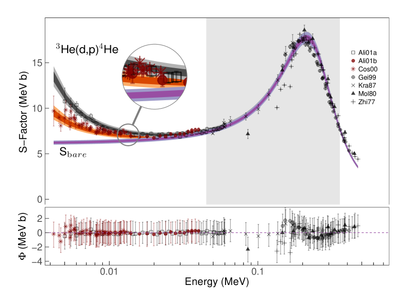
Figure 4: Top Panel: Astrophysical S-factor of ³He(d,p)⁴He for bare and screened nuclei versus center-of-mass energy. The symbols show the different experiments taken into account in the present analysis: open square ($\Box$; Aliotta et al., 2001); red solid circle ($\bullet$; Aliotta et al., 2001); red asterisk ($\ast$; Costantini et al., 2000); circled cross ($\oplus$; Geist et al., 1999); times sign ($\times$; Krauss et al., 1987); solid triangle ($\blacktriangle$; Möller & Besenbacher, 1980); cross (+; Zhichang et al., 1977); see Appendix A for a more detailed discussion. The error bars refer to 68% statistical uncertainties only. The three bands show the results of the present Bayesian analysis: (purple) bare-nucleus S-factor; (red) screened S-factor for the d(³He,p)⁴He reaction; (gray) screened S-factor for the ³He(d,p)⁴He reaction. The shaded areas depict 68%, and 95% credible intervals. The inset shows a magnified view of the region where the three solutions diverge. Bottom panel: The residuals, $\Phi$, (data minus model) of the Bayesian R-matrix model fit. The error bars refer to 99.7% credible intervals around the mean $\Phi$ of each datum.

Figure 5 presents the one- and two-dimensional marginalized posterior densities of the R-matrix parameters and the electron screening potentials. The yellow, green, and purple regions in the diagonal panels depict 68%, 95%, and 99.7% credible intervals of the marginal posterior, while the lower-left triangle displays the pair-wise joint posteriors color-coded accordingly to the local density of sampled points. The dashed contours highlight 68% and 95% joint credible intervals.

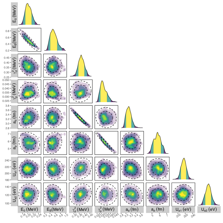
Figure 5: One- and two-dimensional projections of the posterior probability distributions of the R-matrix parameters ($E_{0}$, $E_{B}$, $\gamma_{d}^{2}$, $\gamma_{p}^{2}$, $a_{d}$, $a_{p}$), and electron screening potentials (U_e); see Section 2. The yellow, green, and purple areas on the main diagonal depict 68%, 95%, and 99.7% credible intervals of the marginalized one-dimensional distributions for each parameter. The dashed contours in the lower-left triangle depict 68%, and 95% credible intervals of the two-dimensional pair-wise posterior projections, which is color-coded from yellow to purple with respect to the local density of sampled MCMC points. This triangle plot enables a quick visualization of the covariances between fitted parameters (see, e.g., Bocquet & Carter, 2016).

Summary statistics, i.e., 16th, 50th, and 84th percentiles, for our model parameters are presented in Table 2, together with previous estimates (Coc et al., 2012; Aliotta et al., 2001; Barker, 2007; Descouvemont et al., 2004). For the R-matrix parameters, we obtain values of $E_{0}={0.202}_{-0.0157}^{+0.0184}$ MeV, $E_{B}={0.516}_{-0.135}^{+0.170}$ MeV, $\gamma_{p}^{2}={0.0350}_{-0.0045}^{+0.0067}$ MeV, and $\gamma_{d}^{2}={0.362}_{-0.044}^{+0.048}$ MeV. These uncertainties amount to less than a few percent. The deuteron reduced width is much larger than the proton reduced width, consistent with the structure of the 3/2⁺ level (Section 2). Note that these results cannot be directly compared to the values of Coc et al. (2012), who used fixed boundary conditions and channel radii, and did not provide uncertainties from their $\chi^{2}$ fit.

Table 2: Results of the Bayesian fit. The associated uncertainties in our estimates correspond to a 68% credible interval around the median.

Parameter	Present	Previous
$E_{0}$ (MeV)	${0.202}_{-0.0157}^{+0.0184}$	0.35779
$E_{B}$ (MeV)	${0.516}_{-0.135}^{+0.170}$	0.35779
$\gamma_{p}^{2}$ (MeV)	${0.0350}_{-0.0045}^{+0.0067}$	0.025425
$\gamma_{d}^{2}$ (MeV)	${0.362}_{-0.044}^{+0.048}$	1.0085
$a_{p}$ (fm)	${5.77}_{-0.72}^{+0.67}$	5.0, 5.5 $\pm$ 1.0
$a_{d}$ (fm)	${3.25}_{-0.20}^{+0.21}$	6.0, 5.0
$S_{0}$ (MeV b)	${5.729}_{-0.088}^{+0.097}$	$5.9\pm 0.3$, 6.7
$\sigma_{extr}$ (MeV b)	$0.566\pm 0.029$	✗
Ue1 (eV)	$213\pm 13$	$201\pm 10$, 194, $219\pm 7$
Ue2 (eV)	$121\pm 12$	$146\pm 5$, $109\pm 9$
$\xi_{1}$ (Ali01a)	$1.001\pm 0.014$	✗
$\xi_{2}$ (Ali01b)	$1.021\pm 0.015$	✗
$\xi_{3}$ (Cos00)	$1.063\pm 0.024$	✗
$\xi_{4}$ (Gei99)	$0.969\pm 0.013$	✗
$\xi_{5}$ (Kra87)	$0.986\pm 0.018$	✗
$\xi_{6}$ (Mol80)	$1.005\pm 0.014$	✗
$\xi_{7}$ (Zhi77)	$0.971\pm 0.013$	✗

Table 2 also displays our estimate for the S-factor at zero energy, $S_{0}={5.729}_{-0.088}^{+0.097}$ MeV b, which agrees with the value of Descouvemont & Baye (2010). However, our uncertainty is smaller by about a factor of $3$, which is likely caused by the differences in methodologies and adopted data sets. For the extrinsic scatter, we find a value of $\sigma_{extr}=0.566\pm 0.029$ MeV b. This average value is mainly determined by the datasets from Zhichang et al. (1977); Möller & Besenbacher (1980), which have few significant outliers.

Figure 6 shows the correlations of the predicted S-factor at zero energy, $S_{0}$, with the two channel radii. A stronger correlation is observed with $a_{d}$ compared to $a_{p}$, resulting in a much smaller uncertainty for the former radius. We find values of $a_{d}$ $=$ ${3.25}_{-0.20}^{+0.21}$ fm and $a_{p}$ $=$ ${5.77}_{-0.72}^{+0.67}$ fm. It is interesting to compare our results for the channel radii with the fixed, but arbitrary values that were used in previous analyses. For $a_{d}$, we rule out the previously adopted values of $5$ fm (Barker, 2007), and $6$ fm (Descouvemont et al., 2004) with 95% credibility, while the previously adopted values of $a_{p}$ = $5$ fm (Descouvemont et al., 2004; Barker, 2007), and $a_{p}$ = 5.5 $\pm$ 1.0 fm from Woods et al. (1988) are consistent with our results.

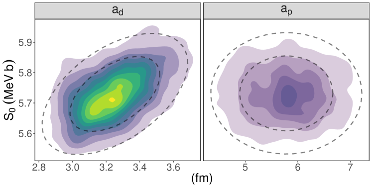
Figure 6: Two-dimensional projections of the posterior probability densities for the predicted S-factor at zero energy ($S_{0}$) versus the channel radii ($a_{d}$,$a_{p}$). The panels and colors have the same meaning as in Figure 4. The correlation with the deuteron channel radius, $a_{d}$ (left panel), is larger compared to the correlation with $a_{p}$ (right panel).

For the screening potentials, we obtain values of $U_{e1}$ $=$ $213\pm 13$ eV for the ³He(d,p)⁴He  reaction, and U_e2 $=$ $121\pm 12$ eV for the d(³He,p)⁴He  reaction. Our result for ³He(d,p)⁴He  is consistent with previous estimates (Aliotta et al., 2001; Descouvemont et al., 2004; Barker, 2007) within 95% credibility. Our estimated screening potential for d(³He,p)⁴He also agrees with Aliotta et al. (2001) and Descouvemont et al. (2004) within the uncertainties. Note that the present and previous estimated values are still larger than the called adiabatic limit, i.e., the difference in electron binding energies between the colliding atoms and the compound atom, $U_{e}=120$ eV for ³He(d,p)⁴He, and $U_{e}=65$ eV for d(³He,p)⁴He (see e.g., Aliotta et al., 2001), and this discrepancy is still not understood.

The posterior densities for the data set normalization factors are displayed in Figure 7 and their summary statistics is presented at the bottom of Table 2. The gray areas depict 68%, 95%, and 99.7% credible intervals. The vertical dashed red line represents zero systematic effects (i.e., a normalization factor of unity). The fitted normalization factors are consistent with unity within 95% credibility, except for the data set of Costantini et al. (2000), for which the median value of $\xi$ differs from unity by 6.3%.

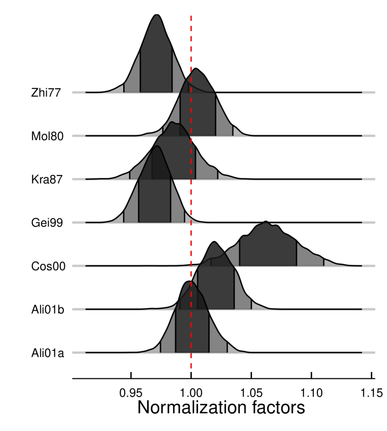
Figure 7: Posteriors of the normalization factors, $\xi_{j}$, for each of the seven data sets. The gray areas depict 68%, 95%, and 99.7% credible intervals, respectively. For the data set labels, see Figure 4.

5 Bayesian Reaction Rates

The thermonuclear reaction rate per particle pair is given by (Iliadis, 2008):

$$N_{A}\left\langle\sigma v\right\rangle =\left(\frac{8}{\pi\mu}\right)^{\frac{1}{2}}\frac{N_{A}}{(k_{B}T)^{\frac{3}{2}}}\int_{0}^{\infty}e^{-2\pi\eta}S(E)e^{-\frac{E}{k_{B}T}}dE,$$ (22)

where $S(E)$ is the bare-nucleus S-factor at the center-of-mass energy $E$, according to Equation 2; $\mu=m_{a}m_{b}/(m_{a}+m_{b})$ is the reduced mass, with $m_{a}$ and $m_{a}$ denoting the masses of target and projectile, respectively; $k_{B}$ is the Boltzmann constant, $N_{A}$ is Avogadro’s constant, and $T$ is the temperature. For calculating the ³He(d,p)⁴He reaction rate, we integrate Equation 22 numerically. The S-factor is calculated from the samples obtained with our Bayesian model, which contains the effects of varying channel radii and boundary condition parameters. Our rate is based on 5,000 MCMC samples, randomly chosen from the complete set of S-factor samples, which ensures that Monte Carlo fluctuations are negligible compared to the rate uncertainties. Our lower integration limit is 10 eV. We estimate the reaction rates on a grid of temperatures from 1 MK to 1 GK. Recommended rates are computed as the 50th percentile of the probability density, while the rate factor uncertainty, $f.u.$, is found from the 16th and 84th percentiles. Numerical reaction rate values are listed in Table 3. Our rate uncertainties amount between 1.1% and 1.7% over the entire temperature region of interest.

Table 3: Recommended ³He(d,p)⁴He reaction rates.

T (GK)	Rate	$f.u.$	T (GK)	Rate	$f.u.$
0.001	3.4959E-19	1.017	0.07	1.0933E+04	1.014
0.002	6.0351E-13	1.017	0.08	2.1937E+04	1.014
0.003	6.2480E-10	1.016	0.09	3.9560E+04	1.014
0.004	4.9259E-08	1.016	0.1	6.5782E+04	1.014
0.005	1.0932E-06	1.016	0.11	1.0274E+05	1.013
0.006	1.1578E-05	1.016	0.12	1.5260E+05	1.013
0.007	7.6001E-05	1.016	0.13	2.1759E+05	1.013
0.008	3.5811E-04	1.016	0.14	2.9999E+05	1.013
0.009	1.3253E-03	1.016	0.15	4.0190E+05	1.013
0.01	4.0848E-03	1.016	0.16	5.2554E+05	1.012
0.011	1.0917E-02	1.016	0.18	8.4624E+05	1.012
0.012	2.6040E-02	1.016	0.2	1.2778E+06	1.012
0.013	5.6610E-02	1.016	0.25	2.9262E+06	1.011
0.014	1.1397E-01	1.016	0.3	5.4933E+06	1.011
0.015	2.1514E-01	1.016	0.35	9.0208E+06	1.011
0.016	3.8445E-01	1.016	0.4	1.3448E+07	1.011
0.018	1.0727E+00	1.016	0.45	1.8653E+07	1.011
0.02	2.5929E+00	1.016	0.5	2.4479E+07	1.011
0.025	1.5146E+01	1.016	0.6	3.7350E+07	1.011
0.03	5.8024E+01	1.015	0.7	5.0858E+07	1.012
0.04	4.0895E+02	1.015	0.8	6.4133E+07	1.012
0.05	1.6354E+03	1.015	0.9	7.6622E+07	1.012
0.06	4.7026E+03	1.015	1.0	8.7989E+07	1.012

Figure 8 compares our present rates with previous estimates. Our 16th and 84th percentiles, divided by our recommended rate (50th percentile), are shown as the gray band. The “lower”, “adopted”, and “upper” rates of Descouvemont et al. (2004) are displayed as the purple band. The solid line depicts the ratio of the previously “adopted” rate and our median (50th percentile) rate. Compared to the present rates, the previous results are slightly higher at temperatures below $10$ MK and lower at $\approx 300$ MK. Previous and present results agree within the uncertainties for the entire temperature range. We emphasize that we achieved a significant reduction of the reaction rate uncertainties, from a previous average value of 3.2% (Descouvemont et al., 2004) to $1.4$% in the present work.

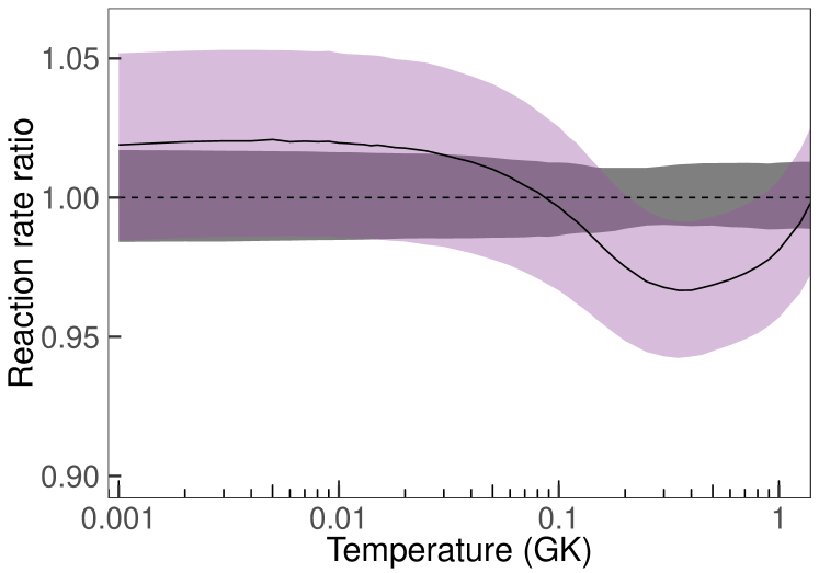
Figure 8: Present ³He(d,p)⁴He thermonuclear reaction rates compared to the evaluation of Descouvemont et al. (2004). The gray shaded area corresponds to our new Bayesian rates, while the purple shaded area depicts the previous rates. The bands depict 68% coverage probabilities. All rates are normalized to the new recommended rate, listed in Table 3. The solid line shows the ratio of the previous and present recommended rates.

6 Summary and Conclusions

Big-Bang nucleosynthesis represents a milestone in the evolution of the Universe, marking the production of the first light nuclides. Accurate estimates of the rates of the nuclear reactions occurring during this period are paramount to predict the primordial abundances of the first elements. Inferring reaction rates from the measured S-factors requires a proper quantification and implementation of the different types of uncertainties affecting the measurement process. If these effects are not taken properly into account, the reaction rate estimate will be biased. The main results of our analysis can be summarized as follows:

• This work represents the first implementation of a hierarchical Bayesian R-matrix formalism, which we applied to the estimation of ³He(d,p)⁴He S-factors and thermonuclear reaction rates.

• The single-level, two-channel R-matrix approximation was incorporated into an adaptive MCMC sampler for robustness against multi-modality and correlations between the R-matrix parameters.

• The Bayesian modeling naturally accounts for all known sources of uncertainties affecting the experimental data: extrinsic scatter, systematic effects, imprecisions in the measurement process, and the effects of electron screening.

• We include the R-matrix parameters (energies, reduced widths, channel radii, and boundary conditions), the data set normalization factors, and the electron screening potential in the fitting process.

• Thermonuclear reaction rates and associated uncertainties are obtained by numerically integrating our Bayesian S-factors. We achieved a significant reduction of the reaction rate uncertainties, from a previous average value of 3.2% (Descouvemont et al., 2004) to $1.4$%. This implies that the big bang ³He abundance can now be predicted with an uncertainty of only 1.0%. Future observations of the primordial ³He abundance will thus provide strong constraints for the standard big-bang model (Cooke, 2015).

Appendix A Nuclear Data for the ³He(d,p)⁴He Reaction

A.1 The ³He(d,p)⁴He data of Zhichang et al. (1977)

The cross section data of Zhichang et al. (1977), as reported in EXFOR (2017), originate from a private communication by the authors and were adopted from Figure 2 of the original article. The derived experimental S-factors, together with their statistical uncertainties ($\approx$ $0.6$%) are listed in Table 4. The estimated systematic uncertainty is $3.4$%, including the effects of target, solid angle, and beam intensity.

Table 4: The ³He(d,p)⁴He data of Zhichang et al. (1977).

$E_{c.m.}\pm\Delta E_{c.m.}$	$S\pm\Delta S_{\mathrm{stat}}\tablenotemark{a}$	$E_{c.m.}\pm\Delta E_{c.m.}$	$S\pm\Delta S_{\mathrm{stat}}\tablenotemark{a}$
(MeV)	(MeV b)	(MeV)	(MeV b)
0.1344 $\pm$ 0.0048	10.074 $\pm$ 0.060	0.2559 $\pm$ 0.0042	15.950 $\pm$ 0.095
0.1422 $\pm$ 0.0047	12.080 $\pm$ 0.072	0.2676 $\pm$ 0.0042	14.505 $\pm$ 0.087
0.1506 $\pm$ 0.0047	12.544 $\pm$ 0.075	0.2736 $\pm$ 0.0041	14.194 $\pm$ 0.085
0.1650 $\pm$ 0.0046	12.375 $\pm$ 0.074	0.2748 $\pm$ 0.0041	14.231 $\pm$ 0.085
0.1677 $\pm$ 0.0045	14.590 $\pm$ 0.087	0.2949 $\pm$ 0.0041	12.757 $\pm$ 0.076
0.1692 $\pm$ 0.0045	15.314 $\pm$ 0.092	0.3186 $\pm$ 0.0041	10.505 $\pm$ 0.063
0.1746 $\pm$ 0.0045	15.760 $\pm$ 0.095	0.3468 $\pm$ 0.0040	9.188 $\pm$ 0.055
0.1800 $\pm$ 0.0044	15.987 $\pm$ 0.096	0.3822 $\pm$ 0.0040	6.773 $\pm$ 0.040
0.1854 $\pm$ 0.0044	17.415 $\pm$ 0.104	0.4110 $\pm$ 0.0039	5.863 $\pm$ 0.035
0.1914 $\pm$ 0.0044	18.116 $\pm$ 0.109	0.4314 $\pm$ 0.0038	5.071 $\pm$ 0.030
0.1974 $\pm$ 0.0044	17.763 $\pm$ 0.107	0.4500 $\pm$ 0.0037	4.695 $\pm$ 0.028
0.2040 $\pm$ 0.0044	17.728 $\pm$ 0.106	0.4710 $\pm$ 0.0037	4.411 $\pm$ 0.026
0.2100 $\pm$ 0.0044	17.825 $\pm$ 0.107	0.5070 $\pm$ 0.0036	3.761 $\pm$ 0.022
0.2247 $\pm$ 0.0043	17.502 $\pm$ 0.105	0.5466 $\pm$ 0.0035	3.002 $\pm$ 0.018
0.2400 $\pm$ 0.0043	16.640 $\pm$ 0.099	0.5772 $\pm$ 0.0034	2.999 $\pm$ 0.018
0.2520 $\pm$ 0.0042	15.987 $\pm$ 0.096	0.6135 $\pm$ 0.0033	2.364 $\pm$ 0.014

A.2 The ³He(d,p)⁴He and d(³He,p)⁴He data of Krauss et al. (1987)

The Krauss et al. (1987) experiments took place at the ion accelerators in Münster and Bochum. Table 3 in Krauss et al. (1987) lists measured S-factors and statistical uncertainties. A normalization uncertainty of 6% originates from an absolute ³He(d,p)⁴He cross section measurement at a center-of-mass energy of $59.66$ keV, to which a 5% uncertainty caused by variations in the alignment of beam and gas jet target profiles has to be added for the Münster data. Hence, we adopt a systematic uncertainty of 6.0% for the Bochum data and, following the authors, a value of 7.8% for the Münster data. Note that Krauss et al. (1987) do not report separately the results for ³He(d,p)⁴He and d(³He,p)⁴He. Since this distinction is important below a center-of-mass energy of $50$ keV, we disregard all of their data points in this energy range. The data adopted in our analysis are listed in Table 5.

Table 5: The ³He(d,p)⁴He and d(³He,p)⁴He data of Krauss et al. (1987).

$E_{c.m.}$	$S\pm\Delta S_{\mathrm{stat}}\tablenotemark{b}$	$E_{c.m.}$	$S\pm\Delta S_{\mathrm{stat}}\tablenotemark{b}$
(MeV)	(MeV b)	(MeV)	(MeV b)
0.04970	7.24 $\pm$ 0.07	0.0830	9.1 $\pm$ 0.4
0.05369	7.67 $\pm$ 0.08	0.1007	9.9 $\pm$ 0.5
0.05900	8.4 $\pm$ 0.4	0.1184	11.5 $\pm$ 0.6
0.05952	7.96 $\pm$ 0.08	0.1360	13.1 $\pm$ 0.6
0.05966	8.26 $\pm$ 0.08	0.1537	16.0 $\pm$ 0.8
0.0653	8.6 $\pm$ 0.5	0.1713	17.2 $\pm$ 0.9

A.3 The d(³He,p)⁴He data of Möller & Besenbacher (1980)

In this experiment, the d(³He,p)⁴He differential cross section was measured at two angles, relative to the d(d,p)³H cross section. The total cross section was calculated using the angular distributions from Yarnell et al. (1953). The statistical error is less than 3%, except at the lowest energy (7%). The systematic error, which arises from the normalization, the d(d,p)³H cross section, and the anisotropy coefficient, amounts to 3.9%. The EXFOR cross section data were presumably scanned from Fig. 3 of (Möller & Besenbacher, 1980). Our adopted S-factors are listed in Table 6.

Table 6: The d(³He,p)⁴He data of Möller & Besenbacher (1980).

$E_{c.m.}$	$S$	${\Delta}S_{\mathrm{stat}}$	${\Delta}S_{\mathrm{sys}}$
(MeV)	(MeV b)	(MeV b)	(MeV b)
0.0856	7.17	0.50	0.28
0.1460	14.18	0.42	0.55
0.1736	16.68	0.50	0.65
0.2056	18.58	0.56	0.72
0.2196	17.24	0.52	0.67
0.2336	17.65	0.53	0.69
0.2668	14.77	0.44	0.58
0.2964	13.22	0.40	0.52
0.3088	11.22	0.34	0.44
0.3280	10.16	0.30	0.40
0.3856	7.34	0.22	0.29
0.4460	5.02	0.15	0.20
0.5064	3.87	0.12	0.15
0.5648	2.885	0.086	0.11
0.6256	2.337	0.070	0.090
0.6836	2.011	0.060	0.080
0.7504	1.681	0.050	0.070
0.8068	1.553	0.046	0.060

A.4 The ³He(d,p)⁴He and d(³He,p)⁴He data of Geist et al. (1999)

The cross section data are presented in Figure 5 of Geist et al. (1999) and are available in tabular form from EXFOR, as communicated by the authors. Three data sets exist, one for the ³He(d,p)⁴He reaction and two for the d(³He,p)⁴He reaction. The data are listed in Table 7, with statistical uncertainties only. We do not distinguish between the ³He(d,p)⁴He and d(³He,p)⁴He reactions because all data points were measured at center-of-mass energies above $50$ keV where electron screening effects can be disregarded. A systematic uncertainty of 4.3% is obtained by adding quadratically the contributions from the d(d,p)³H monitor cross section scale and fitting procedure (1.3% and 3%, respectively), the incident beam energy and energy loss (2%), and the beam integration (2%).

Table 7: The ³He(d,p)⁴He and d(³He,p)⁴He data of Geist et al. (1999).

$E_{c.m.}$	$S\pm\Delta S_{\mathrm{stat}}\tablenotemark{a}$	$E_{c.m.}$	$S\pm\Delta S_{\mathrm{stat}}\tablenotemark{a}$
(MeV)	(MeV b)	(MeV)	(MeV b)
0.1527	15.89 $\pm$ 0.11	0.3344	8.965 $\pm$ 0.033
0.1645	16.76 $\pm$ 0.21	0.3463	8.273 $\pm$ 0.046
0.1762	17.07 $\pm$ 0.14	0.3583	7.640 $\pm$ 0.041
0.1880	17.36 $\pm$ 0.20	0.3702	7.134 $\pm$ 0.045
0.1899	17.418 $\pm$ 0.067	0.3821	6.571 $\pm$ 0.037
0.1999	17.40 $\pm$ 0.15	0.3880	6.309 $\pm$ 0.036
0.2017	17.562 $\pm$ 0.094
0.2117	17.38 $\pm$ 0.23	0.1468	14.64 $\pm$ 0.22
0.2236	16.36 $\pm$ 0.21	0.1702	16.94 $\pm$ 0.23
0.2255	16.635 $\pm$ 0.070	0.1779	16.64 $\pm$ 0.23
0.2374	15.86 $\pm$ 0.12	0.2092	17.02 $\pm$ 0.22
0.2493	15.08 $\pm$ 0.12	0.2170	17.02 $\pm$ 0.22
0.2612	14.12 $\pm$ 0.10	0.2404	15.79 $\pm$ 0.21
0.2732	13.300 $\pm$ 0.045	0.2522	14.903 $\pm$ 0.081
0.2746	13.399 $\pm$ 0.052	0.2542	14.747 $\pm$ 0.059
0.2851	12.181 $\pm$ 0.077	0.2717	13.27 $\pm$ 0.11
0.2866	12.464 $\pm$ 0.083	0.2855	12.68 $\pm$ 0.11
0.2971	11.520 $\pm$ 0.079	0.3029	10.69 $\pm$ 0.14
0.2985	11.428 $\pm$ 0.064	0.3169	10.17 $\pm$ 0.11
0.3089	10.474 $\pm$ 0.090	0.3482	8.012 $\pm$ 0.083
0.3105	10.598 $\pm$ 0.055	0.3795	6.394 $\pm$ 0.074
0.3224	9.6450 $\pm$ 0.053	0.4108	5.351 $\pm$ 0.060

A.5 The d(³He,p)⁴He data of Costantini et al. (2000)

We adopted the d(³He,p)⁴He results of Table 1 in Costantini et al. (2000), which lists the effective energy, S-factor, statistical uncertainty, and systematic uncertainty. The latter ranges from 8% at the lowest energy ($4.22$ keV) to 3.0% at the highest energy ($13.83$ keV). In our analysis, we assume an average systematic uncertainty of 5.5%. Table 8 lists the S-factors adopted in the present work.

Table 8: The d(³He,p)⁴He data of Costantini et al. (2000).

$E_{c.m.}$	$S\pm\Delta S_{\mathrm{stat}}\tablenotemark{a}$	$E_{c.m.}$	$S\pm\Delta S_{\mathrm{stat}}\tablenotemark{a}$
(MeV)	(MeV b)	(MeV)	(MeV b)
0.00422	9.7 $\pm$ 1.7	0.00834	7.51 $\pm$ 0.22
0.00459	9.00 $\pm$ 0.67	0.00851	7.38 $\pm$ 0.22
0.00471	8.09 $\pm$ 0.62	0.00860	7.65 $\pm$ 0.23
0.00500	8.95 $\pm$ 0.70	0.00871	7.82 $\pm$ 0.28
0.00509	9.8 $\pm$ 1.0	0.00898	7.36 $\pm$ 0.19
0.00537	8.86 $\pm$ 0.48	0.00908	7.66 $\pm$ 0.17
0.00544	8.01 $\pm$ 0.39	0.00914	7.60 $\pm$ 0.24
0.00551	9.68 $\pm$ 0.70	0.00929	7.54 $\pm$ 0.23
0.00554	8.87 $\pm$ 0.55	0.00938	7.47 $\pm$ 0.14
0.00577	8.99 $\pm$ 0.31	0.00948	7.59 $\pm$ 0.13
0.00583	8.93 $\pm$ 0.36	0.00978	7.32 $\pm$ 0.22
0.00590	8.74 $\pm$ 0.25	0.00987	7.52 $\pm$ 0.19
0.00593	8.31 $\pm$ 0.55	0.00991	7.24 $\pm$ 0.18
0.00623	8.15 $\pm$ 0.29	0.01007	7.39 $\pm$ 0.19
0.00631	8.10 $\pm$ 0.23	0.01018	7.35 $\pm$ 0.14
0.00652	8.26 $\pm$ 0.48	0.01029	7.44 $\pm$ 0.17
0.00657	8.03 $\pm$ 0.26	0.01087	7.38 $\pm$ 0.16
0.00672	8.32 $\pm$ 0.16	0.01096	7.35 $\pm$ 0.13
0.00700	7.90 $\pm$ 0.27	0.01105	7.41 $\pm$ 0.17
0.00707	8.32 $\pm$ 0.28	0.01165	7.24 $\pm$ 0.14
0.00734	7.70 $\pm$ 0.16	0.01178	7.21 $\pm$ 0.12
0.00740	7.69 $\pm$ 0.15	0.01185	7.35 $\pm$ 0.11
0.00746	7.90 $\pm$ 0.18	0.01241	7.58 $\pm$ 0.14
0.00752	7.83 $\pm$ 0.26	0.01255	7.31 $\pm$ 0.13
0.00812	7.31 $\pm$ 0.11	0.01265	7.31 $\pm$ 0.14
0.00819	7.31 $\pm$ 0.25	0.01307	7.36 $\pm$ 0.13
0.00822	7.43 $\pm$ 0.24	0.01383	7.23 $\pm$ 0.13
0.00829	7.85 $\pm$ 0.24

A.6 The ³He(d,p)⁴He and d(³He,p)⁴He data of Aliotta et al. (2001)

The S-factor data for the ³He(d,p)⁴He and d(³He,p)⁴He reactions are taken from Tables 1 and 2, respectively, in Aliotta et al. (2001). The quoted uncertainties include only statistical (2.6%) effects. The systematic uncertainty arises from the target pressure, calorimeter, and detection efficiency, and amounts to 3.0%. The S-factor data adopted in the present work are listed in Table 9.

Table 9: The ³He(d,p)⁴He and d(³He,p)⁴He data of Aliotta et al. (2001).

$E_{c.m.}$	$S\pm\Delta S_{\mathrm{stat}}\tablenotemark{c}$	$E_{c.m.}$	$S\pm\Delta S_{\mathrm{stat}}\tablenotemark{c}$
(MeV)	(MeV b)	(MeV)	(MeV b)
0.00501	10.8 $\pm$ 1.5	0.02508	7.18 $\pm$ 0.20
0.00550	10.31 $\pm$ 0.81	0.02592	7.17 $\pm$ 0.19
0.00601	9.41 $\pm$ 0.48	0.02662	6.93 $\pm$ 0.18
0.00602	10.37 $\pm$ 0.35	0.02788	7.01 $\pm$ 0.19
0.00645	9.36 $\pm$ 0.35	0.02873	7.22 $\pm$ 0.20
0.00690	8.82 $\pm$ 0.31	0.02988	7.19 $\pm$ 0.19
0.00751	9.12 $\pm$ 0.29	0.02991	6.87 $\pm$ 0.18
0.00780	8.66 $\pm$ 0.28	0.03110	7.24 $\pm$ 0.20
0.00818	8.31 $\pm$ 0.24	0.03190	7.17 $\pm$ 0.19
0.00896	7.85 $\pm$ 0.26	0.03289	7.04 $\pm$ 0.20
0.00902	7.88 $\pm$ 0.22	0.03349	7.33 $\pm$ 0.20
0.00966	7.68 $\pm$ 0.22	0.03389	7.43 $\pm$ 0.20
0.01072	7.48 $\pm$ 0.20	0.03586	7.22 $\pm$ 0.18
0.01144	7.29 $\pm$ 0.20	0.03589	7.39 $\pm$ 0.19
0.01195	7.19 $\pm$ 0.35	0.03589	7.58 $\pm$ 0.20
0.01199	7.35 $\pm$ 0.20	0.03788	7.63 $\pm$ 0.20
0.01318	7.28 $\pm$ 0.20	0.03858	7.33 $\pm$ 0.18
0.01395	6.95 $\pm$ 0.23	0.03987	7.65 $\pm$ 0.20
0.01439	7.04 $\pm$ 0.20	0.04067	7.44 $\pm$ 0.22
0.01499	7.07 $\pm$ 0.20	0.04187	7.29 $\pm$ 0.20
0.01595	6.87 $\pm$ 0.18	0.04306	7.48 $\pm$ 0.22
0.01675	7.16 $\pm$ 0.20	0.04485	7.40 $\pm$ 0.20
0.01794	6.91 $\pm$ 0.19	0.04544	7.70 $\pm$ 0.22
0.01799	7.02 $\pm$ 0.20	0.04786	7.63 $\pm$ 0.20
0.01914	7.20 $\pm$ 0.20	0.05021	7.66 $\pm$ 0.22
0.01993	6.75 $\pm$ 0.18	0.05083	7.70 $\pm$ 0.20
0.02094	6.81 $\pm$ 0.18	0.05265	7.70 $\pm$ 0.22
0.02155	7.09 $\pm$ 0.20	0.05382	7.77 $\pm$ 0.22
0.02192	6.96 $\pm$ 0.19	0.05504	7.77 $\pm$ 0.22
0.02271	7.13 $\pm$ 0.20	0.05681	7.88 $\pm$ 0.20
0.02392	6.92 $\pm$ 0.19	0.05741	7.94 $\pm$ 0.22
0.02393	6.91 $\pm$ 0.18	0.05980	8.12 $\pm$ 0.22

A.7 Other data

The following data sets were excluded from our analysis. Bonner et al. (1952) only present differential cross sections measured at zero degrees. The cross section data of Jarvis & Roaf (1953), obtained using photographic plates, are presented in their Table 1 for three bombarding energies. However, the origin of their quoted errors (6% $-$ 14%) is not clear. Yarnell et al. (1953) report the differential cross section at $86^{\circ}$ (see their Figure 6), but the bombarding energy uncertainty is large (3% $-$ 14%) and the different contributions to the total cross section uncertainty cannot be estimated individually from the information provided. The latter argument also holds for the data of Freier & Holmgren (1954) (see their Figure 1). Arnold et al. (1954) provide cross sections between $36$ keV and $93$ keV bombarding deuteron energy (see their Table 3), including a detailed error analysis. However it was suggested by Coc et al. (2015) that an unaccounted systematic error affected the d(d,n)³He cross section measured in the same experiment. For the data of Kunz (1955), we could not estimate separately the statistical and systematic uncertainty contributions. We disregarded the data of La Cognata et al. (2005) because their indirect method does not provide absolute cross section values. They normalized their results to cross sections obtained in other experiments, mainly the data of Geist et al. (1999). See also the discussion in Barker (2007) regarding the absolute cross section normalization of La Cognata et al. (2005). We did not include the data of Engstler et al. (1988) and Prati et al. (1994) in our analysis because these results are biased by stopping-power problems. Finally, we also did not take into account the results of Barbui et al. (2013), who reported the plasma³He(d,p)⁴He S-factor using intense ultrafast laser pulses. The derivation of the S-factor versus center of mass energy from the measured Maxwellian-averaged cross section at different plasma temperatures is complicated and the systematic effects are not obvious to us.

References

- Aliotta et al. (2001) Aliotta, M., Raiola, F., Gyürky, G., et al. 2001, Nuclear Physics A, 690, 790 . http://www.sciencedirect.com/science/article/pii/S0375947401003669
- Ando et al. (2006) Ando, S., Cyburt, R. H., Hong, S. W., & Hyun, C. H. 2006, Phys. Rev. C, 74, 025809. https://link.aps.org/doi/10.1103/PhysRevC.74.025809
- Andrae et al. (2010) Andrae, R., Schulze-Hartung, T., & Melchior, P. 2010, ArXiv e-prints, arXiv:1012.3754
- Arnold et al. (1954) Arnold, W. R., Phillips, J. A., Sawyer, G. A., Stovall, E. J., & Tuck, J. L. 1954, Phys. Rev., 93, 483. https://link.aps.org/doi/10.1103/PhysRev.93.483
- Assenbaum et al. (1987) Assenbaum, H. J., Langanke, K., & Rolfs, C. 1987, Zeitschrift für Physik A Atomic Nuclei, 327, 461. https://doi.org/10.1007/BF01289572
- Aver et al. (2015) Aver, E., Olive, K. A., & Skillman, E. D. 2015, J. Cosmology Astropart. Phys, 7, 011
- Bania et al. (2002) Bania, T. M., Rood, R. T., & Balser, D. S. 2002, Nature, 415, 54
- Barbui et al. (2013) Barbui, M., Bang, W., Bonasera, A., et al. 2013, Phys. Rev. Lett., 111, 082502. https://link.aps.org/doi/10.1103/PhysRevLett.111.082502
- Barker (2002) Barker, F. 2002, Nuclear Physics A, 707, 277 . http://www.sciencedirect.com/science/article/pii/S0375947402009211
- Barker (1997) Barker, F. C. 1997, Phys. Rev. C, 56, 2646. https://link.aps.org/doi/10.1103/PhysRevC.56.2646
- Barker (2007) —. 2007, Phys. Rev. C, 75, 027601. https://link.aps.org/doi/10.1103/PhysRevC.75.027601
- Bocquet & Carter (2016) Bocquet, S., & Carter, F. W. 2016, The Journal of Open Source Software, 1, doi:10.21105/joss.00046. http://dx.doi.org/10.21105/joss.00046
- Bonner et al. (1952) Bonner, T. W., Conner, J. P., & Lillie, A. B. 1952, Phys. Rev., 88, 473. https://link.aps.org/doi/10.1103/PhysRev.88.473
- Coc et al. (2012) Coc, A., Descouvemont, P., Olive, K. A., Uzan, J.-P., & Vangioni, E. 2012, Phys. Rev. D, 86, 043529. https://link.aps.org/doi/10.1103/PhysRevD.86.043529
- Coc et al. (2015) Coc, A., Petitjean, P., Uzan, J.-P., et al. 2015, Phys. Rev. D, 92, 123526. https://link.aps.org/doi/10.1103/PhysRevD.92.123526
- Coc & Vangioni (2010) Coc, A., & Vangioni, E. 2010, Journal of Physics: Conference Series, 202, 012001. http://stacks.iop.org/1742-6596/202/i=1/a=012001
- Cooke (2015) Cooke, R. J. 2015, ApJ, 812, L12. http://stacks.iop.org/2041-8205/812/i=1/a=L12
- Cooke et al. (2018) Cooke, R. J., Pettini, M., & Steidel, C. C. 2018, ApJ, 855, 102
- Costantini et al. (2000) Costantini, H., Formicola, A., Junker, M., et al. 2000, Physics Letters B, 482, 43 . http://www.sciencedirect.com/science/article/pii/S037026930000513X
- Cyburt et al. (2016) Cyburt, R. H., Fields, B. D., Olive, K. A., & Yeh, T.-H. 2016, Rev. Mod. Phys., 88, 015004. https://link.aps.org/doi/10.1103/RevModPhys.88.015004
- de Souza et al. (2015) de Souza, R. S., Hilbe, J. M., Buelens, B., et al. 2015, MNRAS, 453, 1928
- de Souza et al. (2016) de Souza, R. S., Dantas, M. L. L., Krone-Martins, A., et al. 2016, MNRAS, 461, 2115
- deBoer et al. (2017) deBoer, R. J., Görres, J., Wiescher, M., et al. 2017, Rev. Mod. Phys., 89, 698
- Descouvemont et al. (2004) Descouvemont, P., Adahchour, A., Angulo, C., Coc, A., & Vangioni-Flam, E. 2004, Atomic Data and Nuclear Data Tables, 88, 203
- Descouvemont & Baye (2010) Descouvemont, P., & Baye, D. 2010, Reports on Progress in Physics, 73, 036301
- Dover et al. (1969) Dover, C. B., Mahaux, C., & Weidenmüller, H. A. 1969, Nuclear Physics A, 139, 593 . http://www.sciencedirect.com/science/article/pii/0375947469902814
- Engstler et al. (1988) Engstler, S., Krauss, A., Neldner, K., et al. 1988, Physics Letters B, 202, 179 . http://www.sciencedirect.com/science/article/pii/0370269388900032
- EXFOR (2017) EXFOR. 2017. http://www.nndc.bnl.gov/exfor/exfor.htm
- Freier & Holmgren (1954) Freier, G., & Holmgren, H. 1954, Physical Review, 93, 825
- Gamow (1948) Gamow, G. 1948, Nature, 162, 680
- Geist et al. (1999) Geist, W. H., Brune, C. R., Karwowski, H. J., et al. 1999, Phys. Rev. C, 60, 054003. https://link.aps.org/doi/10.1103/PhysRevC.60.054003
- Gelman & Hill (2006) Gelman, A., & Hill, J. 2006, Data Analysis Using Regression and Multilevel/Hierarchical Models, Analytical Methods for Social Research (Cambridge University Press), doi:10.1017/CBO9780511790942
- Gelman & Rubin (1992) Gelman, A., & Rubin, D. B. 1992, Statist. Sci., 7, 457. http://dx.doi.org/10.1214/ss/1177011136
- Gómez Iñesta et al. (2017) Gómez Iñesta, A., Iliadis, C., & Coc, A. 2017, ApJ, 849, 134. http://stacks.iop.org/0004-637X/849/i=2/a=134
- González-Gaitán et al. (2019) González-Gaitán, S., de Souza, R. S., Krone-Martins, A., et al. 2019, Monthly Notices of the Royal Astronomical Society, 482, 3880. http://dx.doi.org/10.1093/mnras/sty2881
- Hale et al. (2014) Hale, G. M., Brown, L. S., & Paris, M. W. 2014, Physical Review C, 89, 014623
- Hartig et al. (2018) Hartig, F., Minunno, F., & Paul, S. 2018, BayesianTools: General-Purpose MCMC and SMC Samplers and Tools for Bayesian Statistics, r package version 0.1.5. https://CRAN.R-project.org/package=BayesianTools
- Heinrich & Lyons (2007) Heinrich, J., & Lyons, L. 2007, Annual Review of Nuclear and Particle Science, 57, 145. https://doi.org/10.1146/annurev.nucl.57.090506.123052
- Hilbe et al. (2017) Hilbe, J. M., de Souza, R. S., & Ishida, E. E. O. 2017, Bayesian Models for Astrophysical Data Using R, JAGS, Python, and Stan, doi:10.1017/CBO9781316459515
- Iliadis (2008) Iliadis, C. 2008, Nuclear Physics of Stars, Physics textbook (Wiley). https://books.google.com/books?id=rog9FxfGZQoC
- Iliadis et al. (2016) Iliadis, C., Anderson, K. S., Coc, A., Timmes, F. X., & Starrfield, S. 2016, ApJ, 831, 107. http://stacks.iop.org/0004-637X/831/i=1/a=107
- Jarvis & Roaf (1953) Jarvis, R., & Roaf, D. 1953, Proceedings of the Royal Society of London A: Mathematical, Physical and Engineering Sciences, 218, 432. http://rspa.royalsocietypublishing.org/content/218/1134/432
- Jaynes & Bretthorst (2003) Jaynes, E., & Bretthorst, G. 2003, Probability Theory: The Logic of Science (Cambridge University Press). https://books.google.com/books?id=tTN4HuUNXjgC
- Krauss et al. (1987) Krauss, A., Becker, H., Trautvetter, H., Rolfs, C., & Brand, K. 1987, Nuclear Physics A, 465, 150 . http://www.sciencedirect.com/science/article/pii/0375947487903022
- Kunz (1955) Kunz, W. E. 1955, Physical Review, 97, 456
- La Cognata et al. (2005) La Cognata, M., Spitaleri, C., Tumino, A., et al. 2005, Phys. Rev. C, 72, 065802. https://link.aps.org/doi/10.1103/PhysRevC.72.065802
- Lane & Thomas (1958) Lane, A. M., & Thomas, R. G. 1958, Rev. Mod. Phys., 30, 257. https://link.aps.org/doi/10.1103/RevModPhys.30.257
- Lane & Thomas (1958) Lane, A. M., & Thomas, R. G. 1958, Rev. Mod. Phys., 30, 257. https://link.aps.org/doi/10.1103/RevModPhys.30.257
- Long & de Souza (2018) Long, J. P., & de Souza, R. S. 2018, Statistical Methods in Astronomy (American Cancer Society), 1–11. https://onlinelibrary.wiley.com/doi/abs/10.1002/9781118445112.stat07996
- Loredo (2013) Loredo, T. J. 2013, in Astrostatistical Challenges for the New Astronomy, Edited by Joseph M. Hilbe. Springer, 2013, p. 1013, p. 14-50, ed. J. M. Hilbe, 1013
- Möller & Besenbacher (1980) Möller, W., & Besenbacher, F. 1980, Nuclear Instruments and Methods, 168, 111
- Parent & Rivot (2012) Parent, E., & Rivot, E. 2012, Introduction to Hierarchical Bayesian Modeling for Ecological Data, Chapman & Hall/CRC Applied Environmental Statistics (Taylor & Francis). https://books.google.com/books?id=YYt-ZUTvbjUC
- Peebles & Ratra (2003) Peebles, P. J., & Ratra, B. 2003, Reviews of Modern Physics, 75, 559
- Pitrou et al. (2018) Pitrou, C., Coc, A., Uzan, J.-P., & Vangioni, E. 2018, Physics Reports, arXiv:1801.08023
- Planck Collaboration et al. (2016) Planck Collaboration, Adam, R., Ade, P. A. R., et al. 2016, A&A, 594, A1
- Prati et al. (1994) Prati, P., Arpesella, C., Bartolucci, F., et al. 1994, Zeitschrift für Physik A Hadrons and Nuclei, 350, 171. https://doi.org/10.1007/BF01290685
- Riess et al. (1998) Riess, A. G., Filippenko, A. V., Challis, P., et al. 1998, AJ, 116, 1009
- Savage et al. (1999) Savage, M. J., Scaldeferri, K. A., & Wise, M. B. 1999, Nuclear Physics A, 652, 273
- Sbordone et al. (2010) Sbordone, L., Bonifacio, P., Caffau, E., et al. 2010, A&A, 522, A26. https://doi.org/10.1051/0004-6361/200913282
- Spergel et al. (2007) Spergel, D. N., Bean, R., Doré, O., et al. 2007, ApJS, 170, 377
- Team R Development Core (2010) Team R Development Core. 2010, R: A language and environment for statistical computing, R Foundation for Statistical Computing, Vienna, Austria. http://www.r-project.org
- ter Braak & Vrugt (2008) ter Braak, C. J. F., & Vrugt, J. A. 2008, Statistics and Computing, 18, 435. https://doi.org/10.1007/s11222-008-9104-9
- Thomas (1951) Thomas, R. G. 1951, Phys. Rev., 81, 148. https://link.aps.org/doi/10.1103/PhysRev.81.148
- Tilley et al. (2002) Tilley, D., Cheves, C., Godwin, J., et al. 2002, Nuclear Physics A, 708, 3 . http://www.sciencedirect.com/science/article/pii/S0375947402005973
- Wigner & Eisenbud (1947) Wigner, E. P., & Eisenbud, L. 1947, Physical Review, 72, 29
- Woods et al. (1988) Woods, C. L., Barker, F. C., Catford, W. N., Fifield, L. K., & Orr, N. A. 1988, Australian Journal of Physics, 41, 525
- Yarnell et al. (1953) Yarnell, J. L., Lovberg, R. H., & Stratton, W. R. 1953, Physical Review, 90, 292
- Zhichang et al. (1977) Zhichang, L., Jingang, Y., & Xunliang, D. 1977, Atom. Ener. Sci. Tech., 129